Approximations and asymptotics of upper hedging prices in multinomial models
Abstract
We give an exposition and numerical studies of upper hedging prices in multinomial models from the viewpoint of linear programming and the game-theoretic probability of Shafer and Vovk. We also show that, as the number of rounds goes to infinity, the upper hedging price of a European option converges to the solution of the Black-Scholes-Barenblatt equation.
Keywords: Black-Scholes-Barenblatt equation, contingent claim, Cox-Ross-Rubinstein formula, incomplete market, stochastic control, trinomial model.
1 Introduction
The Black-Scholes formula for the geometric Brownian motion model and the Cox-Ross-Rubinstein formula for the binomial model are now treated in many standard textbooks on mathematical finance (e.g. [13, 21, 22]). Since these models are complete, the exact price for any contingent claim is determined by arbitrage argument. On the other hand, incomplete models such as the trinomial model are only briefly mentioned in the textbooks because of difficulty associated with indeterminacy of prices of contingent claims.
In fact only a few explicit results seem to be known on upper hedging prices for the discrete-time multinomial models. The purpose of this paper is to give an exposition of the exact and the asymptotic behavior of upper hedging prices of contingent claims in multinomial models. We also show that the asymptotic upper hedging price of a European option is described by the Black-Scholes-Barenblatt equation (e.g. [1], [26], [9], [12], Chapter 4 of [15]). The Black-Scholes-Barenblatt equation is usually considered for uncertain volatility models in continuous time and its relation to multinomial models does not seem to be stated in literature.
The advantage of discrete-time multinomial models is that we can exactly compute the upper hedging price by backward induction for moderate number of rounds and various approximations to the upper hedging price can be compared to the exact value. Basic facts on the upper hedging price for discrete models are well explained in Chapter 4 of the first edition of Musiela and Rutkowski [13]. General treatments of incomplete markets are given in Chapter 5 of [10] and [18]. However they are concerned with continuous stochastic processes and do not contain much numerical information on the behavior of upper hedging prices for discrete models.
An extensive numerical study of hedging in incomplete markets is given in [3]. Its authors consider a hedging strategy which minimizes the mean-squared error to the payoff of a contingent claim under Markov-state dynamics. As we see in Section 2 below, for studying the behavior of upper hedging prices we can not make convenient stochastic assumptions such as the Markov property. Results more relevant to the present paper have been given in [17] and [5] by convex ordering argument. In particular for discrete time models with bounded martingale differences, [17] proves that the upper hedging price of a convex contingent claim is given by the extremal binomial model. We reproduce this fact in Proposition 2.4 below by linear programming argument.
In this paper we use the framework of game-theoretic probability by Shafer and Vovk. We prefer the framework because of the following reasons. First, in game-theoretic probability only the protocol of a game between “Investor” and “Market” is formulated without specification of a probability measure. Therefore there is no need to distinguish a risk neutral measure from an actual (or a physical) measure and to consider the equivalence between them. This is advantageous because the extremal risk neutral measure corresponding to the upper hedging price usually has a support smaller than those in the interior of the set of risk neutral measures. Second, some strong properties of a price path of Market can be proved in game-theoretic probability without any stochastic assumption (e.g. see [25], [27], [28] and references therein). As a referee pointed out [4] studies non-probabilistic approach for pricing in continuous time. Third, the notion of upper hedging price is of central importance to game-theoretic probability as shown in our recent works ([24], [20]) on game-theoretic probability.
The organization of the paper is as follows. In Section 2 we give a linear programming formulation of upper hedging prices in multinomial models and state some basic facts in several propositions. In Section 3 we give some simple bounds for upper hedging prices. Then in Section 4 we show that, as the number of rounds goes to infinity, the upper hedging price of a European option converges to the solution of an additive form of the Black-Scholes-Barenblatt equation. In Section 5 we present numerical studies on the accuracy of the partial differential equation and other approximations. Some concluding remarks are given in Section 6.
2 Formulation of upper hedging price
In this section we formulate the upper hedging price for a multinomial game from the viewpoint of linear programming and the game-theoretic probability of Shafer and Vovk [19]. Also we show some known facts on upper hedging prices.
Let be a finite set containing both negative and positive elements. The protocol of the multinomial game of rounds with the initial capital of is written as follows.
FOR .
Investor announces .
Market announces .
.
END FOR
We call the sample space and a path of Market’s moves. For , is a partial path. Investor’s strategy is a function specifying based on :
with some initial value , where denotes the initial empty path. When Investor adopts , his capital at the end of round is written as , where
We can write the progression of the game in a rooted tree with the root . For , is an intermediate node branching to , . The final nodes are .
We call a function a payoff function or a contingent claim. The upper hedging price (or simply the upper price) of is defined as
and the lower hedging price is defined as
| (1) |
The upper hedging price and the lower hedging price are often called seller’s price and buyer’s price, respectively. A strategy with the initial capital satisfying , is called a superreplicating strategy for .
The problem of obtaining the upper hedging price can be formulated in linear programming. Let . For the single step case , is obtained as the following minimum:
| (2) |
For the two-step case , Investor can choose his investment at round 2 depending on the Market’s move in the first round. Therefore is written as the following minimum:
For general , the coefficient matrix is recursively defined as
where is a -dimensional vector of 1’s, is without the first column and denotes the Kronecker product. Then
| (3) |
where is a -dimensional vector consisting of , and
Since the size of grows exponentially with , it becomes difficult to directly solve the linear programming problem for a general path-dependent contingent claim . Exploiting the recursive structure of the coefficient matrix , the linear programming problem can be solved by backward induction, i.e. by solving the single-step optimizations for . This will be explicitly described in (8) below. Therefore the single-step optimization in (2) is essential. However even with backward induction, for a general path-dependent , the number of single-step optimizations grows exponentially with . This is because the number of nodes of the game tree grows exponentially with and the single-step optimization for the backward induction is performed at each node of the game tree. This difficulty is somewhat mitigated in the case of a European option , where is a function of only. Then the game tree can be collapsed according to the values of and the number of nodes of the collapsed tree grows only polynomially with . In fact, for generic values of , the number of values taken by is .
Now we consider the single-step optimization in (2). Let contain negative elements and positive elements, which are ordered as
Note that we allow the case , which needs some special consideration. For the single-step game the following result is given in Proposition 4.1.1 of [13]. We give our own proof based on consideration of dual linear programming problem to (2).
Proposition 2.1.
The upper hedging price of in the single-step game is given by
| (4) |
Proof.
Let and consider the following dual problem to (2):
| (5) |
Note that the coefficient matrix is . Therefore the maximum is attained by a basic solution involving two variables.
First consider the case . If we choose two variables either from or from , then the solution does not satisfy and it is infeasible. Therefore for a feasible basic solution we need to choose one variable from and another variable from . Then the basic solution is given by
| (6) |
and the value of the objective function is given by .
By (1) the lower hedging price for the single-step game is given as
The vector satisfying (5) is a probability vector over such that its expectation is zero:
Let denote the set of probability vectors satisfying (5). is called a risk neutral measure on . From (5) we have , where denotes the usual expectation under . This duality is well known in great generality (see Chapter 5 of [10]). However the explicit expression of the upper hedging price in (4) is useful for the purpose of numerical backward induction for .
Remark 2.2.
We can also consider the dual problem to (3) for the -step problem. It is easy to see that the set of risk neutral measures is characterized as follows:
| (7) | ||||
Also by duality we have . Note that (7) holds even if for some and some conditional probabilities on the right-hand side are not defined. At each node of the game tree, the conditional distribution of the extremal risk neutral measure corresponding to is given by a basic solution of the form (4).
Based on (4), the backward induction for obtaining for the -step game is described as follows. Define , , by
| (8) |
with the initial condition , . Summarizing the arguments above we have the following proposition.
Proposition 2.3.
The upper hedging price of in the -step game is given by
Consider the case that the payoff is defined on the whole . Then we have the following result.
Proposition 2.4.
Suppose that is convex. Then is given by the binomial model concentrated on two outermost values . For the case is given by the binomial model concentrated on two innermost values . For the case .
This result was proved by Rüschendorf ([17]) by a convex ordering argument in a more general setting, where is a bounded interval. See also [5]. Corresponding results for concave are obtained by using (1). We now give a simple proof of this proposition using (8).
Proof.
First consider the one-step game . By convexity of it is easy to check that for any and the following inequalities hold:
Hence the proposition holds for the single-step game.
For we can use the induction. We note that is a convex combination of , , where the weights of the combination are given by the binomial model and they do not depend on . In particular is convex in . ∎
Remark 2.5.
As pointed out in Remark 2 of [17], the above result holds if is component-wise convex in every , .
3 Some bounds for upper hedging prices
In this section we present some simple inequalities for upper hedging prices.
We first investigate the relation between binomial model and general multinomial model. Pick a negative element and a positive element from and restrict the move space of Market to the two element set . Then the multinomial game is reduced to a binomial model, where the price of any contingent claim is given by an arbitrage argument. Let denote the price of under the binomial model . For the two-element set there is no need to take the maximum in (8). On the other hand, for a multinomial model we take the maximum in (8) at each node of the game. This gives the following lower bound for :
| (9) |
Similarly for the lower hedging price we have
The above inequalities can be generalized by considering nested move spaces of Market. Explicitly writing in the multinomial game, let and denote the upper hedging price and the lower hedging price of multinomial game with as Market’s move space. Consider two nested move spaces of Market. Then the same consideration as above gives the following inequalities:
| (10) |
In Section 5 we compare upper and lower hedging prices in trinomial and quadnomial models.
We can also consider dynamic restrictions of the move space of Market. For example, we can consider the maximization in (8) only for even and use the maximizer from this round for the subsequent round . Or we can maximize e.g. every 10th step. By this dynamic restriction we again have a lower bound for the upper hedging price. As we discuss in the next section, this pruning of maximizations is conceptually close to discretization of partial differential equation in (13).
We now present another bound when is a European option depending only on . Let be defined on the whole . Assume that has the first derivative which is of bounded variation. Then is written as a difference of two non-decreasing functions (Section 5.2 of [16]). By taking the indefinite integral of we see that is written as a sum of a convex function and a concave function:
By the subadditivity of the upper hedging price (Section 8.3 of [19]), we have
| (11) |
4 Limiting behavior of upper hedging price of an European option
In this section we derive the limit of the upper hedging price of a European option as in an appropriate sequence of games. Let denote the space of functions with compact support and continuous second derivatives. Let . We consider a sequence of multinomial games with rounds, where the payoff for the -th game is given as
| (12) |
Note that the expected value under the two-point distribution in (6) is zero and the variance is given as
In view of this define the maximum variance and the minimum variance of as
We now state the following theorem.
Theorem 4.1.
Let and let be defined by (12). Assume . Then
where , , , satisfies the following partial differential equation
| (13) |
with the boundary condition .
Similarly the following partial differential equation describes the limiting lower price of .
| (14) |
We can understand (13) as a piecewise heat equation, where the diffusion coefficient depends on the convexity or concavity of . As pointed out by a referee the equation (13) is studied in [14].
We stated Theorem 4.1 for the simple setting of and . Theorem 4.6.9 of [15] states that the Black-Scholes-Barenblatt equation holds for a payoff function with linear growth condition: for some , , . In view of this result we expect our Theorem 4.1 also holds for continuous satisfying a linear growth condition. However justifying the limiting argument from discrete time to continuous time does not seem to be simple.
Remark 4.2.
The case needs a special consideration, although Theorem 4.1 still holds for this case. In view of Theorem 4.6.9 of [15], the notion of viscosity solution (cf. [7]) is needed for (13).
In Section 6.3 of [19] this case was treated using parabolic potential theory. The equivalence of (13) to the treatment in Section 6.3 of [19] is seen by the following intuitive argument. If , then , , and is non-decreasing in . strictly increases in at some if and only if is strictly convex in at this point. Then for all , is (at least weakly) convex in . This implies that if and only if , which corresponds to the “continuous region” in Section 6.3 of [19].
Note that (13) is an additive form of the Black-Scholes-Barenblatt equation in which the right-hand side of (13) multiplied by :
| (15) |
Consider a multiplicative model, where Reality chooses positive ’s and is the product of ’s. A European option is of the form . In (20) below we see that the resulting partial differential equation is exactly the Black-Scholes-Barenblatt equation. Note that the multiplicative model is standard in finance literature, although it is well known that the pioneering work of Bachelier ([2]) was formulated in the additive form. In this paper we use additive model, because game-theoretic protocols are usually formulated in an additive form and also because the limiting partial differential equation is a more direct generalization of the heat equation.
A rigorous proof of our theorem is somewhat tedious and we first give some heuristic arguments as to why (13) should hold. Later we give a more formal proof, by considering an approximate superreplicating strategy as in Section 6.2 of [19].
For our argument it is more convenient to rescale the move space of Market in the -th game to
| (16) |
After this rescaling, the backward induction in (8) for the -th game is written as
| (17) |
where and are given by (6). The initial condition is given by . Note that by backward induction (17) defines for all , since is defined on the whole .
As in the proof of Proposition 2.4 is a convex combination of values . It should be noted that, unlike the case of convex in Proposition 2.4, the weights of the convex combination depend on . However as seen from the proof of Proposition 2.4, the weights are concentrated either on the two outermost values or on the two innermost values , depending on the convexity of in . Hence in each interval of convexity or concavity of , it is twice continuously differentiable in . In our numerical studies we found that if the payoff function is smooth and has only finite number of inflection points, then as a function of has no more inflection points than .
Write . Then each term in the right-hand side of (17) is expanded as
where derivatives are with respect and uniformly in and . Then (17) is written as
| (18) |
If we ignore , the right hand side is maximized by or depending on the sign of .
Now by rescaling time axis define
Then (18) is written as
| (19) |
This clearly corresponds to (13). However it seems difficult to let in (19) and prove our theorem directly, although the finite difference approximation to HJB equations in Chapter IX of [8] should hold in some form.
At this point we indicate how the Black-Scholes-Barenblatt equation (15) arises in the multiplicative case. In the multiplicative multinomial model, is assumed to be of the form , where is given in (16). Let . Then
The expansion of the right-hand side of (17) in the multiplicative model is
| (20) |
This corresponds to (15).
Instead of the above direct approach, knowing that (13) should hold, we can construct an approximate superreplicating strategy of Investor and prove our theorem as in Section 6.2 of [19]. In the following proof, in order to show the inequality we adopt a suggestion by a referee.
Proof of Theorem 4.1.
By Theorem 4.6.9 of [15], the solution to (13) has a continuous first-order derivative in and a continuous second-order derivative in . See also Theorem 11 of [9] and [26]. Consider the following sequence
where . Writing , , , we can expand the successive difference as
| (21) |
where is uniformly in and . Consider a Markov superhedging strategy (cf. [9]) of Investor which chooses . By adding (21) for we have
| (22) |
At this point we adopt a suggestion by a referee. From Proposition 2.1 and Remark 2.2 we know that the upper hedging price is computed as the expected value of under the extremal risk neutral measure, say . Under any risk neutral measure, , , is a measure-theoretic martingale and its expected value is zero. Now consider the expected value of
under . We can evaluate the expected value, first by conditioning on . By the definition of , under the conditional variance of satisfies
Therefore taking the unconditional expected value of (22) under we have except for a term of order . Hence .
Conversely, consider Market’s randomized moves chosen according to the extremal risk neutral measure corresponding to , which is concentrated to two outermost values or two innermost values at each node of the game tree, depending on the sign of (see Remark 2.2). Investor’s capital is a measure-theoretic martingale under this risk neutral measure. Since the measure is supported on two points at each node of the game tree, we can modify the standard argument for binomial models to show that the expected value of the payoff converges to under the measure. On the other hand is the supremum over all possible moves of Market. Therefore we have . ∎
Remark 4.3.
In the above proof we partly used measure theoretic arguments as suggested by a referee. Although we can give a purely game theoretic proof in the line of Section 6.2 of [19], it is somewhat tedious. The difficulty lies in the fact that is path-dependent. Note that by the game-theoretic law of large numbers ([19], [11]), Investor can force that converge to 0. This implies that for large the empirical distribution of Market’s moves is approximately a risk neutral measure and is the variance of a risk neutral measure. However because each is multiplied by , the convergence does not imply
Although the argument can be fixed by discretization of the values of , we omit the details.
Numerically (13) can be solved by the following backward induction: 1) discretization of the interval and , 2) approximation of the second derivative by the second order difference of three neighboring points. Actually this backward induction is entirely similar to the exact backward induction in (8). When the discretization is not fine enough, then the above numerical approximation corresponds to pruning of maximizations discussed in Section 3. This suggests that a coarse discretization of the partial differential equation yields an approximation which is less than the the true .
5 Numerical examples
In this section we check results of this paper by numerical computation.
We first calculate the upper hedging price and the lower hedging price of Butterfly spread option in Figure 1 under the trinomial model . Although Butterfly spread does not satisfy the differentiability condition of Theorem 4.1, it can be arbitrarily closely approximated by a payoff function satisfying the condition of Theorem 4.1. The results are shown in Figure 2 in conjunction with the price under the binomial models. From Figure 2, we see that the upper price and the lower price are different from the price under the binomial models.


We now add a new Market’s move to the trinomial model and compare the former trinomial model to this quadnomial model. We consider the following three values of as depicted in Figure 3.
- 1.
“outside”.
- 2.
“middle”.
- 3.
“inside”.

Figures 6, 6, 6 show the upper hedging prices of the butterfly spread for these quadnomial models compared to those of the trinomial model. In Figure 6 the upper hedging prices under the quadnomial model equal those under the trinomial model with increasing , whereas in Figures 6, 6 the upper hedging prices under the quadnomial models differ from those under the trinomial model.


Next we consider the payoff , which has a lot of changes from convexity to concavity, and similarly calculate the upper hedging prices. The results are shown in Figures 9, 9, 9. Also in this case the upper hedging prices under the quadnomial model equal those under the trinomial model with increasing , provided that .


Next, we vary the values of from 0 to 5 by . Figure 10 displays the plot of the upper hedging prices of the butterfly spread for and . From Figure 10, we see that the upper hedging prices converge to an equal value in the interval .
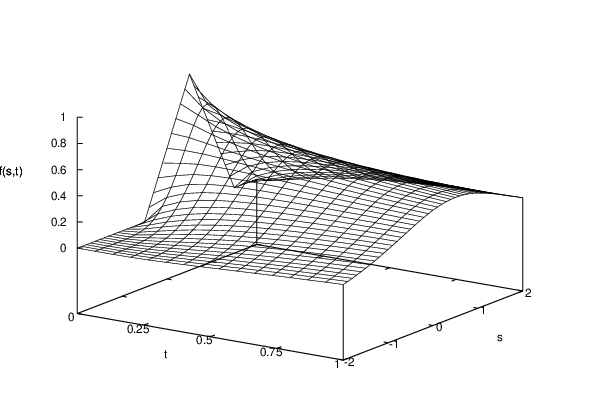
Finally Figure 12 shows a numerical solution to the partial differential equation (13) for and for the case of Butterfly spread . We compute an approximation of by the following difference scheme:
| (23) |
We rewrite (23) as
| (24) |
We set and (13). For discretization we use and , which satisfies the stability condition (Section 8.4 of [29] or page 47 of [23])
for discretization of the heat equation Since our partial differential equation (13) can be understood as a piecewise heat equation, in our numerical experiments we found that and satisfying the same stability condition works well. With and , we obtain and using difference scheme (24). In Figure 12, we compute (14) for the lower prices by the similar difference method. Table 1 shows the upper prices and the lower prices obtained in Figure 2. We find that these converge to the values obtained by the difference method for the partial differential equations (13) and (14).

| upper price | lower prices | |
|---|---|---|
| 1 | 0.2500 | 0.0000 |
| 20 | 0.3824 | 0.1926 |
| 40 | 0.3790 | 0.1993 |
| 60 | 0.3820 | 0.2012 |
| 80 | 0.3799 | 0.2032 |
| 100 | 0.3807 | 0.2032 |
6 Concluding remarks
In this paper we discussed various approximations and asymptotics of upper hedging prices in multinomial models. In particular we showed that, as the number of rounds goes to infinity, the upper hedging price of a European option converges to the solution of an additive form of the Black-Scholes-Barenblatt equation. By numerical experiments we checked that this convergence is fast and the asymptotic approximation is useful.
A multinomial model is the simplest example of incomplete market. A natural extension of a multinomial model is the bounded forecasting game ([19]), where Market’s move is a bounded interval containing the origin. This problem was already considered in [17]. Most results of this paper can be extended to the bounded forecasting game.
Usually the Black-Scholes-Barenblatt equation is studied in the case of vector-valued processes. Then the maximum variance and the minimum variance are no longer uniquely determined and the maximization in each step of the game tree is more complicated. Numerical studies of vector-valued cases are left to our future investigation.
Acknowledgments. The authors are grateful to two reviewers for their careful reading and constructive comments. We thank Takayasu Matsuo for very useful comments on numerical solution of the partial differential equation and Hitoshi Ishii for his very kind explanation on existence of the classical solution or the viscosity solution of the partial differential equation.
References
- [1] M. Avellaneda and R. Buff. Combinatorial implications of nonlinear uncertain volatility models: The case of barrier options. Appl. Math. Finance, 6, 1–18, 1998.
- [2] Louis Bachelier, M. H. A. Davis and Alison Etheridge. Louis Bachelier’s Theory of Speculation : The Origins of Modern Finance., Princeton University Press, Princeton, 2006.
- [3] Dimitris Bertsimas, Leonid Kogan and Andrew W. Lo. Hedging derivative securities and incomplete markets: an -arbitrage approach. Operations Research, 49, 372–397, 2001.
- [4] A. Bick and W. Willinger. Dynamic spanning without probabilities. Stochastic Processes and their Applications, 50, 349–374, 1994.
- [5] C. Courtois and M. Denuit. Convex bounds on multiplicative processes, with applications to pricing in incomplete markets. Insurance: Mathematics and Economics, 42, 95–100, 2008.
- [6] John C. Cox, Stephen A. Ross, and Mark Rubinstein. Option pricing: A simplified approach. Journal of Financial Economics, 3, 229–263, 1979.
- [7] Michael G. Crandall, Hitoshi Ishii and Pierre-Louis Lions. User’s guide to viscosity solutions of second order partial differential equations. Bull. Amer. Math. Soc., 27, 1–67, 1992.
- [8] Wendell H. Fleming and H. Mete Soner. Controlled Markov Processes and Viscosity Solutions, 2nd ed., Springer-Verlag, New York, 2006.
- [9] Fausto Gozzi and Tiziano Vargiolu. Superreplication of European multiasset derivatives with bounded stochastic volatility. Mathematical Methods of Operations Research, 55, 69–91, 2002.
- [10] I. Karatzas and S. E. Shreve. Methods of Mathematical Finance. Springer-Verlag, New York, 1998.
- [11] M. Kumon and A. Takemura. On a simple strategy weakly forcing the strong law of large numbers in the bounded forecasting game. Annals of the Institute of Statistical Mathematics, 60, 801–812, 2008.
- [12] Gunter H. Meyer. The Black Scholes Barenblatt equation for options with uncertain volatility and its application to static hedging. International Journal of Theoretical and Applied Finance, 9, 673–703, 2006.
- [13] Marek Musiela and Marek Rutkowski. Martingale Methods in Financial Modelling. 1st edition, Springer-Verlag, Berlin, 1997.
- [14] Shige Peng. -expectation, -Brownian motion and related stochastic calculus of Itô type. Stochastic Analysis and Applications, 541–567, Abel Symp., vol.2, Springer, Berlin, 2007.
- [15] Huyên Pham. Continuous-time Stochastic Control and Optimization with Financial Applications, Springer, Berlin, 2009.
- [16] H. L. Royden. Real Analysis. 3rd ed., Prentice Hall, New Jersey, 1988.
- [17] L. Rüschendorf. On upper and lower prices in discrete time models. Proceedings of the Steklov Institute of Mathematics, 237, 134–139, 2002.
- [18] Walter Schachermayer. Portfolio optimization in incomplete financial markets. Notes of the Scuola Normale Superiore Cattedra Galileiana, Pisa, 2004.
- [19] Glenn Shafer and Vladimir Vovk. Probability and Finance: It’s Only a Game! Wiley, New York, 2001.
- [20] Glen Shafer, Vladimir Vovk and Akimichi Takemura. Levy’s zero-one law in game-theoretic probability. arXiv:0905.0254v1 [math.PR]. Submitted for publication.
- [21] S. E. Shreve. Stochastic Calculus for Finance I – The Binomial Asset Pricing Model. Springer-Verlag, New York, 2003.
- [22] S. E. Shreve. Stochastic Calculus for Finance II – Continuous-Time Models. Springer-Verlag, New York, 2005.
- [23] G. D. Smith. Numerical Solutions of Partial Differential Equations, 3rd ed., Clarendon Press, Oxford, 1985.
- [24] Akimichi Takemura, Vladimir Vovk and Glenn Shafer. The generality of the zero-one laws. Annals of the Institute of Statistical Mathematics, doi:10.1007/s10463-009-0262-0, 2009.
- [25] Kei Takeuchi, Masayuki Kumon and Akimichi Takemura. A new formulation of asset trading games in continuous time with essential forcing of variation exponent. Bernoulli, 15, 1243–1258, 2009.
- [26] Tiziano Vargiolu. Existence, uniqueness and smoothness for the Black-Scholes-Barenblatt equation. University of Padova, Department of Pure and Applied Mathematics, Rapporto Interno no.5, http://www.math.unipd.it/˜vargiolu/BSB.pdf. 2001.
- [27] Vladimir Vovk. Rough paths in idealized financial markets. Lithuanian Mathematical Journal, 51, 274–285, 2011.
- [28] Vladimir Vovk. Continuous-time trading and the emergence of probability. To appear in Finance and Stochastics, 2011.
- [29] Paul Wilmott, Sam Howison, and Jeff Dewynne. The Mathematics of Financial Derivatives. Cambridge University Press, Cambridge, 1995.