跳到论文正文
W Papers独立论文阅读器 arXiv:1007.4361 论文正文 计算阅读时间 · 0%
引用这篇论文根据当前论文元数据生成,正式投稿前建议核对。


License: arXiv.org perpetual non-exclusive license
arXiv:1007.4361v2 [q-fin.PR] 06 Apr 2012

Spectral Decomposition of Option Prices in Fast Mean-Reverting Stochastic Volatility Models

Jean-Pierre Fouque ††thanks: Department of Statistics & Applied Probability, University of California, Santa Barbara, CA 93106-3110, fouque@pstat.ucsb.edu. Work partially supported by NSF grant DMS-0806461.    Sebastian Jaimungal ††thanks: Department of Statistics, University of Toronto, Toronto, Ontario M5S 3G3, sebastian.jaimungal@utoronto.ca. Work partially supported by NSERC.    Matthew J. Lorig ††thanks: ORFE Department, Princeton University, Sherrerd Hall, Princeton NJ 08544, mlorig@princeton.edu.
August 24, 2026
Abstract

Using spectral decomposition techniques and singular perturbation theory, we develop a systematic method to approximate the prices of a variety of European and path-dependent options in a fast mean-reverting stochastic volatility setting. Our method is shown to be equivalent to those developed in [10], but has the advantage of being able to price options for which the methods of [10] are unsuitable. In particular, we are able to price double-barrier options. To our knowledge, this is the first time that double-barrier options have been priced in a stochastic volatility setting in which the Brownian motions driving the stock and volatility are correlated.

1 Introduction

Since it was originally analyzed in the context of Sturm-Liouville operators, spectral theory has enjoyed wide popularity in both science and engineering. In physics, for example, the stationary-state wave functions are simply the eigenfunctions of the time-independent Schrödinger equation. And, electrical engineers are well-versed in the theory of Fourier series and Fourier transforms. It is not surprising then, that techniques from spectral theory have found their place in finance as well.

For instance, in [23] eigenfunction methods are used to price European-style options in a Black-Scholes setting. The authors of [16] use eigenfunction techniques in the context of bond pricing. Spectral decomposition techniques have been particularly successful at aiding in the development of analytic pricing formulas for a variety of exotic options. For example, in [30], Fourier series methods are used to obtain closed-form expressions for prices of double-barrier options in the Black-Scholes setting. And in [8, 25, 26] spectral decomposition techniques are used to obtain analytic option prices–both European and path-dependent–where the underlying and short rate are controlled by a one-dimensional diffusion. Additionally, the authors of [27] use spectral methods to evaluate both bonds and options in a unified credit-equity framework.

Like spectral theory, stochastic volatility models have become an indispensable tool in mathematical finance. By and large, this is due to the fact that two of the earliest and most well-known stochastic volatility models–the Heston model [19] and Hull-White model [22]–capture the most salient features of the implied volatility surface while at the same time maintaining analytic tractability. Stochastic volatility models have become so popular, in fact, that entire books have been written on the subject [10, 15, 24].

It seems natural, then, to try to employ elements from spectral theory in a stochastic volatility setting. Yet, other than the spectral decomposition of various volatility processes, which is expertly done in [24], there is a surprising lack of literature in this area. In particular, we are unaware of any literature that uses spectral methods to price double-barrier options in a stochastic volatility setting in which the Brownian motions driving the stock and volatility are correlated. The difficulty with using spectral analysis when the stock price and volatility are correlated arises because spectral decomposition techniques work best when there is some sort of symmetry inherent in the problem being studied. This symmetry is broken when the stock price and volatility are correlated via two Brownian motions. Yet we know that correlation between the stock price and the volatility is important because it is needed in order to capture the skew of the implied volatility at the money and reflect the leverage effect [10, 15].

In this paper, we apply techniques from spectral theory to a class of fast mean-reverting stochastic volatility models in which the stock price and volatility are correlated via two Brownian motions. The two-dimensional diffusion that controls the stock and volatility is in contrast to the work of [7, 26, 25, 8, 28], where spectral and probabilistic methods are used to price options on scalar diffusions. Extensions to two-dimensions are highly non-trivial and it is this that distinguishes our work from the earlier contributions. The class of fast mean-reverting stochastic volatility models, first studied in [10], is an important class of models to consider because volatility has been empirically shown to operate on short time-scales [11, 20]. To price options in this setting we employ the singular perturbation methods of [10], but we do this in the context of a spectral expansion.

The rest of this paper proceeds as follows. In section 2.1 we introduce the class of fast mean-reverting stochastic volatility models first considered in [10]. Additionally, we discuss how this class this class of models relates to two of the more popular models used in practice – SABR and Heston. In section 2.2 we present an option-pricing framework, which allows us to consider both European, single- and double-barrier options. This framework results in an option-pricing partial differential equation (PDE) along with appropriate boundary conditions (BC’s), which must be solved in order to specify the price of an option. We briefly mention how the authors of [10] use singular perturbation theory to obtain an approximate solution to the option-pricing PDE and explain why for certain options (e.g. double-barrier options) this methodology is unsuitable. We then present a new method of solving the option-pricing PDE – one which is suitable in cases where the methods of [10] are not. In this new method we assume a solution of a specific form and show how this leads to an eigenvalue equation. An approximate solution to the eigenvalue equation is given in section 3.1. Then, using this solution, we provide formulas for the approximate price of an option in section 3.2. Equivalence of the option-pricing formulas presented in this paper to those derived in [10] is established in section 3.3, as is the accuracy of our pricing approximation. In section 4 we discuss the practical implementation of our methods. We present three examples: European calls, up-and-out calls, and double-barrier knock-out calls. Additionally, we mention how our framework can be extended to price knock-in and rebate options. We finish by discussing some issues related to calibration.

2 A Class of Models and an Outline of Our Method

In this section we introduce a class of fast mean-reverting stochastic volatility models. We then present an option-pricing problem and outline our method for obtaining an approximate solution to this problem.

2.1 A Class of Fast Mean-Reverting Stochastic Volatility Models

We study the class of fast mean-reverting stochastic volatility models first considered by Fouque et al. in [10]. Specifically, under the risk-neutral pricing measure ℙ\mathbb{P}, we consider a non-dividend paying asset (stock, index, etc.) St=exp⁡(Xt)S_{t}=\exp\left(X_{t}\right) whose dynamics are given by the following system of stochastic differential equations (SDE’s)

d​Xt\displaystyle dX_{t} =(μ−12​f2​(Ytϵ))​d​t+f⁡(Ytϵ)​d​Wt,\displaystyle=\left(\mu-\frac{1}{2}f^{2}(Y_{t}^{\epsilon})\right)dt+f(Y_{t}^{\epsilon})\,dW_{t}, (2.1)
d​Ytϵ\displaystyle dY^{\epsilon}_{t} =(1ϵ​(y¯−Ytϵ)−υ​2ϵ​Λ​(Ytϵ))​d​t+υ​2ϵ​d​Bt,\displaystyle=\left(\frac{1}{\epsilon}\left(\overline{y}-Y^{\epsilon}_{t}\right)-\frac{\upsilon\sqrt{2}}{\sqrt{\epsilon}}\Lambda(Y^{\epsilon}_{t})\right)dt+\frac{\upsilon\sqrt{2}}{\sqrt{\epsilon}}\,dB_{t}, (2.2)
d​⟨W,B⟩t\displaystyle d\left\langle W,B\right\rangle_{t} =ρ​d​t.\displaystyle=\rho\,dt. (2.3)

Here, WtW_{t} and BtB_{t} are Brownian motions under ℙ\mathbb{P} with instantaneous correlation ρ\rho such that ρ2≤1\rho^{2}\leq 1. The price process StS_{t} follows a geometric Brownian motion with growth rate μ\mu, which equals to the risk-free rate of interest, and with stochastic volatility f⁡(Ytϵ)f(Y^{\epsilon}_{t}) (the traditional symbol for the risk-free rate of interest rr is reserved for a different purpose). The dynamics of Xt=log⁡StX_{t}=\log S_{t} are obtained from Ito’s Lemma. We note that, as it should be, the discounted stock price (e−μ​t​St)\left(e^{-\mu t}S_{t}\right) is a martingale with respect to the canonical filtration of the Brownian motions. The process YtϵY^{\epsilon}_{t} evolves as an Ornstein-Uhlenbeck (OU) process under the physical measure ℙ~\widetilde{\mathbb{P}}. That is

d​Ytϵ\displaystyle dY^{\epsilon}_{t} =1ϵ​(y¯−Ytϵ)​d​t+υ​2ϵ​d​B~t.(under physical measure ℙ~)\displaystyle=\frac{1}{\epsilon}\left(\overline{y}-Y^{\epsilon}_{t}\right)dt+\frac{\upsilon\sqrt{2}}{\sqrt{\epsilon}}\,d\widetilde{B}_{t}.\qquad\text{(under physical measure $\widetilde{\mathbb{P}}$)} (2.4)

However, under the risk-neutral measure the dynamics of YtϵY^{\epsilon}_{t} acquire a market price of volatility risk, which is given by Λ⁡(Ytϵ)\Lambda(Y^{\epsilon}_{t}). The superscript on YtϵY^{\epsilon}_{t} indicates that this process evolves on a time-scale ϵ\epsilon. The parameter ϵ\epsilon is intended to be small (i.e. 0<ϵ≪10<\epsilon\ll 1) so that the rate of mean-reversion of the OU process is large. It is in this sense that the volatility is fast mean-reverting. We note that under the physical measure, YtϵY^{\epsilon}_{t} has a unique invariant distribution Y∞ϵ∼𝒩⁡(y¯,υ2)Y_{\infty}^{\epsilon}\sim{\cal N}(\overline{y},\upsilon^{2}).

It is not necessary to specify the precise form of f⁡(y)f(y) or Λ⁡(y)\Lambda(y), as only certain moment will play a role in the asymptotic analysis that follows. Likewise, the particular choice of YtϵY_{t}^{\epsilon} as an OU process is not crucial for our analysis. However, in order to guarantee the accuracy of our pricing approximation we need the following assumptions:

  1. 1.

    Under the physical measure, YtϵY_{t}^{\epsilon} has a unique invariant distribution, which is independent of ϵ\epsilon.

  2. 2.

    Under the physical measure, the moments of YtϵY_{t}^{\epsilon} are uniformly bounded in tt. Note that this assumption actually follows from the previous assumption.

  3. 3.

    The smallest non-zero eigenvalue of ℒYϵ{\cal L}_{Y}^{\epsilon} – the infinitesimal generator of YtϵY_{t}^{\epsilon} under the physical measure – is strictly positive.

  4. 4.

    There exists a constant CΛ>0C_{\Lambda}>0 such that |Λ⁡(y)|<CΛ|\Lambda(y)|<C_{\Lambda}.

  5. 5.

    The function f⁡(y)f(y) is such that the solution ϕ⁡(y)\phi(y) of Poisson equation (3.16) is at most polynomially growing.

We note that the Cox–Ingersoll–Ross (CIR) process, as well as the OU process satisfy the above assumptions.

Of practical interest is how two of the most popular stochastic volatility models – Heston and SABR – fit within the fast mean-reverting class of models discussed in this paper. The Heston model [19] can be accommodated in this class by choosing YtϵY_{t}^{\epsilon} to be a CIR process under the physical measure, choosing f⁡(y)=yf(y)=\sqrt{y}, and setting Λ⁡(y)=0\Lambda(y)=0. The rate of mean-reversion of the CIR process should then be scaled by 1/ϵ1/\epsilon and the “volatility of volatility” term should be scaled by 1/ϵ1/\sqrt{\epsilon}. This will ensure that the invariant distribution is independent of ϵ\epsilon. Note that the choice Λ⁡(y)=0\Lambda(y)=0 is not really a restriction on the Heston model as the stochastic variance YtϵY^{\epsilon}_{t} in Heston is a CIR process under both the physical and risk-neutral measures.

The key change between the Black-Scholes model [3] and the Heston model is that the constant volatility of Black-Scholes is replaced by the square-root of a CIR process in Heston. In this sense, the Heston model is essentially an extension of the Black-Scholes model. As such, the CIR process that controls the volatility in the Heston model can be treated as a perturbation around geometric Brownian motion with constant volatility, just as the fast mean-reverting factor of volatility is treated as a perturbation around constant volatility geometric Brownian motion in this paper. This is the reason that the Heston model fits within the fast mean-reverting stochastic volatility framework.

Contrary to Heston, the SABR model [17] is an extension of the Constant-Elastic-Variance (CEV) model [6]. As such, the SABR model does not fit within the class of models considered in this paper. That said, an extension of the CEV model that includes a fast mean-reverting factor of volatility is possible. Approximate option prices for the CEV model with a fast mean-reverting factor of volatility are derived using singular perturbation theory in [5]. Also note, because option prices in the CEV framework have a spectral representation [8], the combined singular perturbation and spectral method developed in this paper would be suitable for CEV with a fast mean-reverting factor of volatility. However, this is outside the scope of the present work.

2.2 Statement of the Option Pricing Problem and Outline of our Method

In this section we introduce an option-pricing problem and outline our method of obtaining an approximate solution to this problem.

Consider an option expiring at time T<∞T<\infty whose payoff can be expressed

Payoff =h⁡(Xτ),\displaystyle=h\left(X_{\tau}\right), τ\displaystyle\tau =inf{t≥0:Xt∉I}∧T,\displaystyle=\inf\{t\geq 0:X_{t}\notin I\}\wedge T, (2.5)
I\displaystyle I :=(l,r),\displaystyle:=(l,r), −∞\displaystyle-\infty ≤l<r≤∞,\displaystyle\leq l<r\leq\infty, (2.6)
h\displaystyle h :I∪{l}∪{r}→ℝ+,\displaystyle:I\cup\left\{l\right\}\cup\left\{r\right\}\rightarrow\mathbb{R}_{+}, h⁡(l)\displaystyle h(l) =h⁡(r)=0,\displaystyle=h(r)=0, (2.7)

In words, the option has payoff h⁡(XT)h(X_{T}) if XX does not leave the interval II prior to time TT, otherwise the option payoff is zero. We use the convention inf{∅}=∞\inf\left\{\emptyset\right\}=\infty. Options that fit within the above payoff framework include European and knock-out style options. But, we shall see in section 4.4 that our results can be extended to include knock-in and rebate style options as well.

We introduce a money market account Mt=eμ​tM_{t}=e^{\mu t}, which we shall use as our option-pricing numéraire. According to risk-neutral pricing, the value of the option PsϵP^{\epsilon}_{s} at time s≤Ts\leq T is given by

PsϵMs\displaystyle\frac{P^{\epsilon}_{s}}{M_{s}} =𝔼⁡[h⁡(Xτ)Mτ|ℱs],\displaystyle=\mathbb{E}\left[\frac{h\left(X_{\tau}\right)}{M_{\tau}}\bigg|{\cal F}_{s}\right], ℱs\displaystyle{\cal F}_{s} =σ({Xt,Ytϵ:0≤t≤s}).\displaystyle=\sigma\left(\left\{X_{t},Y^{\epsilon}_{t}:0\leq t\leq s\right\}\right). (2.8)

After a bit of algebra, and using the Markov property of (X,Yϵ)\left(X,Y^{\epsilon}\right) one finds

Psϵ\displaystyle P^{\epsilon}_{s} =𝕀{τ<s}eμ⁡(s−τ)h(Xτ)+𝔼[e−μ⁡(τ−s)h(Xτ)𝕀{τ≥s}|ℱs]\displaystyle=\mathbb{I}_{\left\{\tau<s\right\}}e^{\mu(s-\tau)}h\left(X_{\tau}\right)+\mathbb{E}\left[e^{-\mu(\tau-s)}h\left(X_{\tau}\right)\mathbb{I}_{\left\{\tau\geq s\right\}}\Big|{\cal F}_{s}\right] (2.9)
=𝕀{τ<s}eμ⁡(s−τ)h(Xτ)+𝕀{τ≥s}Pϵ(s,Xs,Ysϵ),\displaystyle=\mathbb{I}_{\left\{\tau<s\right\}}e^{\mu(s-\tau)}h\left(X_{\tau}\right)+\mathbb{I}_{\left\{\tau\geq s\right\}}P^{\epsilon}\left(s,X_{s},Y^{\epsilon}_{s}\right), (2.10)

where

Pϵ​(s,Xs,Ysϵ)\displaystyle P^{\epsilon}\left(s,X_{s},Y^{\epsilon}_{s}\right) =𝔼[e−μ⁡(τs−s)h(Xτs)|Xs,Ysϵ],\displaystyle=\mathbb{E}\left[e^{-\mu(\tau^{s}-s)}h\left(X_{\tau^{s}}\right)\Big|X_{s},Y^{\epsilon}_{s}\right], (2.11)

and

τs\displaystyle\tau^{s} =inf{t≥s:Xt∉I}∧T.\displaystyle=\inf\{t\geq s:X_{t}\notin I\}\wedge T. (2.12)

We note that the first term in (2.10) is zero as XτX_{\tau} is either equal to ll or rr on the set {τ<s}\left\{\tau<s\right\} and h⁡(l)=h⁡(r)=0h(l)=h(r)=0. Thus, the price of the option at time ss is given simply by the second term of (2.10). From (2.11), one deduces that the function Pϵ​(s,x,y)P^{\epsilon}(s,x,y) solves the following PDE and BC’s (see e.g. Chapter 99 of [29])

0\displaystyle 0 =(∂s−μ+ℒX,Yϵ)Pϵ,\displaystyle=\left(\partial_{s}-\mu+{\cal L}_{X,Y}^{\epsilon}\right)P^{\epsilon}, (s,x,y)∈[0,T]×I×ℝ,\displaystyle(s,x,y)\in[0,T]\times I\times\mathbb{R}, (2.13)
h⁡(x)\displaystyle h(x) =Pϵ​(T,x,y),\displaystyle=P^{\epsilon}(T,x,y), (2.14)
0\displaystyle 0 =Pϵ​(s,l,y),\displaystyle=P^{\epsilon}(s,l,y), ifl>−∞,\displaystyle\text{if}\quad l>-\infty, (2.15)
0\displaystyle 0 =Pϵ​(s,r,y),\displaystyle=P^{\epsilon}(s,r,y), ifr<∞.\displaystyle\text{if}\quad r<\infty. (2.16)

Note that BC’s (2.15) and (2.16) are not required if ll or rr are infinite. The notation ℒX,Yϵ{\cal L}_{X,Y}^{\epsilon} represents the infinitesimal generator of (X,Yϵ)\left(X,Y^{\epsilon}\right). For clarity, we write ℒX,Yϵ{\cal L}_{X,Y}^{\epsilon} explicitly and state its domain 𝒟{\cal D}

ℒX,Yϵ\displaystyle{\cal L}_{X,Y}^{\epsilon} =1ϵ((y¯−y)∂y+υ2∂y​y2)+1ϵ(ρυ2f(y)∂x​y2−υ2Λ(y)∂y)\displaystyle=\frac{1}{\epsilon}\left(\left(\overline{y}-y\right)\partial_{y}+\upsilon^{2}\partial^{2}_{yy}\right)+\frac{1}{\sqrt{\epsilon}}\left(\rho\upsilon\sqrt{2}f(y)\partial^{2}_{xy}-\upsilon\sqrt{2}\Lambda(y)\partial_{y}\right) (2.17)
+(μ−12f2(y))∂x+12f2(y)∂x​x2,\displaystyle\qquad+\left(\mu-\frac{1}{2}f^{2}(y)\right)\partial_{x}+\frac{1}{2}f^{2}(y)\partial^{2}_{xx}, (2.18)
𝒟\displaystyle{\cal D} =I×ℝ.\displaystyle=I\times\mathbb{R}. (2.19)

To simplify subsequent calculations we introduce uϵ​(t,x,y)u^{\epsilon}(t,x,y) such that

Pϵ​(s,x,y)\displaystyle P^{\epsilon}(s,x,y) =e−μ​t​uϵ​(t,x,y),\displaystyle=e^{-\mu t}u^{\epsilon}(t,x,y), t\displaystyle t =T−s.\displaystyle=T-s. (2.20)

A straightforward substitution shows that uϵ​(t,x,y)u^{\epsilon}(t,x,y) satisfies the following PDE and BC’s

0\displaystyle 0 =(−∂t+ℒX,Yϵ)uϵ,\displaystyle=\left(-\partial_{t}+{\cal L}_{X,Y}^{\epsilon}\right)u^{\epsilon}, (t,x,y)∈[0,T]×I×ℝ,\displaystyle(t,x,y)\in[0,T]\times I\times\mathbb{R}, (2.21)
h⁡(x)\displaystyle h(x) =uϵ​(0,x,y),\displaystyle=u^{\epsilon}(0,x,y), (2.22)
0\displaystyle 0 =uϵ​(t,l,y)\displaystyle=u^{\epsilon}(t,l,y) ifl>−∞,\displaystyle\text{if}\quad l>-\infty, (2.23)
0\displaystyle 0 =uϵ​(t,r,y)\displaystyle=u^{\epsilon}(t,r,y) ifr<∞.\displaystyle\text{if}\quad r<\infty. (2.24)

We set uϵ​(t,x,y)=0u^{\epsilon}(t,x,y)=0 for x∉Ix\notin I. Although uϵ​(t,x,y)u^{\epsilon}(t,x,y) is in fact the un-discounted price of an option with time-to-maturity t=T−st=T-s, from this point onward we shall refer to uϵ​(t,x,y)u^{\epsilon}(t,x,y) simply as the price. For convenience, the theorems derived in section 3.2 are given in terms of uϵ​(t,x,y)u^{\epsilon}(t,x,y), as are the examples provided in section 4. The reader should keep in mind that the true price of an option Pϵ​(s,x,y)P^{\epsilon}(s,x,y) at time ss can be recovered from uϵ​(t,x,y)u^{\epsilon}(t,x,y) using (2.20).

In [10] the authors use singular perturbation techniques to find an approximate solution to PDE (2.21) by expanding uϵ​(t,x,y)u^{\epsilon}(t,x,y) in powers of the small parameter ϵ\sqrt{\epsilon}

uϵ\displaystyle u^{\epsilon} =u(0)+ϵ​u(1)+ϵ​u(2)+….\displaystyle=u^{(0)}+\sqrt{\epsilon}\,u^{(1)}+\epsilon\,u^{(2)}+\ldots. (2.25)

Roughly speaking, the authors of [10] show

  1. 1.

    The functions u(0)u^{(0)} and u(1)u^{(1)} are independent of yy.

  2. 2.

    The the 𝒪⁡(ϵ0){\cal O}\left(\epsilon^{0}\right) price is given by u(0)​(t,x)=uB​S​(t,x)u^{(0)}(t,x)=u^{BS}(t,x), where uB​S​(t,x)u^{BS}(t,x) is the Black-Scholes price of an option (with an appropriate level of volatility).

  3. 3.

    The the 𝒪⁡(ϵ1/2){\cal O}\left(\epsilon^{1/2}\right) price u(1)u^{(1)} solves ℒB​S​u(1)=𝒜(1)​uB​S{\cal L}^{BS}u^{(1)}={\cal A}^{(1)}u^{BS}, where ℒB​S=(−∂t+ℒX){\cal L}^{BS}=\left(-\partial_{t}+{\cal L}_{X}\right) is the Black-Scholes pricing operator, ℒX{\cal L}_{X} is defined in (3.63) and 𝒜(1){\cal A}^{(1)} is a linear operator defined in (3.19).

For European-style options – for which uϵ​(t,x,y)u^{\epsilon}(t,x,y) must satisfy only BC (2.22) – and for single-barrier options – for which uϵ​(t,x,y)u^{\epsilon}(t,x,y) must satisfy only BC’s (2.22) and one of either (2.23) or (2.24) – the method of [10] works well because in these cases there exist analytic formulas for uB​S​(t,x)u^{BS}(t,x). However, for double-barrier options – for which uϵ​(t,x,y)u^{\epsilon}(t,x,y) must satisfy all three BC’s (2.22), (2.23) and (2.24) — the methods of [10] are problematic because the Black-Scholes price of a double-barrier option must be expressed as an infinite series [30].

In this paper, we use a combination of singular perturbation techniques and spectral methods to solve PDE (2.21) with BC’s (2.22) - (2.24). The spectral method is outlined as follows: suppose we have the solution to the following eigenvalue equation

ℒX,Yϵ​Ψqϵ\displaystyle{\cal L}_{X,Y}^{\epsilon}\Psi_{q}^{\epsilon} =λqϵ​Ψqϵ.\displaystyle=\lambda_{q}^{\epsilon}\Psi_{q}^{\epsilon}. (2.26)
0\displaystyle 0 =Ψqϵ​(l,y)\displaystyle=\Psi_{q}^{\epsilon}(l,y) ifl>−∞,\displaystyle\text{if}\quad l>-\infty, (2.27)
0\displaystyle 0 =Ψqϵ​(r,y)\displaystyle=\Psi_{q}^{\epsilon}(r,y) ifr<∞.\displaystyle\text{if}\quad r<\infty. (2.28)

By “solution to the eigenvalue equation” we mean that we have the full set of eigenvalues λqϵ\lambda_{q}^{\epsilon} and corresponding eigenfunctions Ψqϵ​(x,y)\Psi_{q}^{\epsilon}(x,y) for which which equations (2.26) - (2.28) are satisfied. Then it is clear that any linear combination of functions of the form eλqϵ​t​Ψqϵ​(x,y)e^{\lambda_{q}^{\epsilon}t}\Psi_{q}^{\epsilon}(x,y) will satisfy PDE (2.21) and BC’s (2.23) and (2.24). Hence, as long as the eigenfunctions allow us enough flexibility to match BC (2.22), the function uϵ​(t,x,y)u^{\epsilon}(t,x,y) can be expressed as 11 1 For simplicity we have assumed either a purely discrete or absolutely continuous spectrum. In fact, depending on the operator ℒX,Yϵ{\cal L}_{X,Y}^{\epsilon} and the BC’s, the spectrum may be discrete, absolutely continuous or mixed. However, in this paper we do not endeavor to solve the full eigenvalue problem (2.26)-(2.28). Rather, we use singular perturbation techniques to find an approximate solution to (2.26)-(2.28). For the asymptotic analysis we perform in section 3.1 we shall need to consider only discrete or continuous spectra.

uϵ​(t,x,y)\displaystyle u^{\epsilon}(t,x,y) ={∑nAnϵ​gnϵ​(t)​Ψnϵ​(x,y)(discrete spectrum)∫Aνϵ​gνϵ​(t)​Ψνϵ​(x,y)​𝑑ν(continuous spectrum),\displaystyle=\begin{cases}\sum_{n}A_{n}^{\epsilon}g_{n}^{\epsilon}(t)\Psi_{n}^{\epsilon}(x,y)&\text{(discrete spectrum)}\\ \int A_{\nu}^{\epsilon}\,g_{\nu}^{\epsilon}(t)\,\Psi_{\nu}^{\epsilon}(x,y)\,d\nu&\text{(continuous spectrum)}\end{cases}, gqϵ​(t)\displaystyle g_{q}^{\epsilon}(t) =exp⁡(λqϵ​t),\displaystyle=\exp\left(\lambda_{q}^{\epsilon}t\right), (2.29)

where qq is a place-holder for either nn or ν\nu and AqϵA_{q}^{\epsilon} are constants to be determined by the payoff.

The main advantage of the spectral method is that by separating the spatial variables (x,y)(x,y) from the temporal variable tt the BC’s (2.23) and (2.24) can be dealt with at the level of the eigenfunctions Ψnϵ​(x,y)\Psi_{n}^{\epsilon}(x,y) as in (2.27) and (2.28), rather than at the level of option prices uϵ​(t,x,y)u^{\epsilon}(t,x,y) as in (2.23) and (2.24). This method is particularly advantageous for pricing double-barrier options.

Using representation (2.29), what remains in order to specify the price of an option is to find expressions for Ψqϵ​(x,y)\Psi_{q}^{\epsilon}(x,y), λqϵ\lambda_{q}^{\epsilon} and AqϵA_{q}^{\epsilon}. This is the subject of section 3.

3 Asymptotic Analysis

An outline of the asymptotic analysis performed in this section is as follows. First, in section 3.1 we derive an approximate solution to eigenvalue equation (2.26). The key results of this derivation are presented in Theorem 3.1, Proposition 3.2 and Theorem 3.3. Next, in section 3.2 we use the results of section 3.1 to derive an expression for the approximate price of an option. This expression, which is given explicitly in Theorem 3.4, serves as the main result of this paper. In section 3.3, we prove that our method of obtaining the approximate price of an option is equivalent to the method of [10]. We summarize this equivalence in Theorems 3.6 and 3.7. Finally, in Theorem 3.8 we also establish the accuracy of our pricing approximation for the case of European options.

3.1 Asymptotic Solution to the Eigenvalue Equation ℒX,Yϵ​Ψqϵ=λqϵ​Ψqϵ{\cal L}_{X,Y}^{\epsilon}\Psi_{q}^{\epsilon}=\lambda_{q}^{\epsilon}\Psi_{q}^{\epsilon}

For general f⁡(y)f(y) and Λ⁡(y)\Lambda(y) there is no analytic solution to the eigenvalue equation ℒX,Yϵ​Ψqϵ=λqϵ​Ψqϵ{\cal L}_{X,Y}^{\epsilon}\Psi_{q}^{\epsilon}=\lambda_{q}^{\epsilon}\Psi_{q}^{\epsilon}. However, we note that ℒX,Yϵ{\cal L}_{X,Y}^{\epsilon} can be conveniently decomposed in powers of ϵ\sqrt{\epsilon} as

ℒX,Yϵ\displaystyle{\cal L}_{X,Y}^{\epsilon} =1ϵ​ℒ(−2)+1ϵ​ℒ(−1)+ℒ(0),\displaystyle=\frac{1}{\epsilon}{\cal L}^{(-2)}+\frac{1}{\sqrt{\epsilon}}{\cal L}^{(-1)}+{\cal L}^{(0)}, (3.1)
ℒ(−2)\displaystyle{\cal L}^{(-2)} =(y¯−y)∂y+υ2∂y​y2,\displaystyle=\left(\overline{y}-y\right)\partial_{y}+\upsilon^{2}\partial^{2}_{yy}, (3.2)
ℒ(−1)\displaystyle{\cal L}^{(-1)} =ρυ2f(y)∂x​y2−υ2Λ(y)∂y,\displaystyle=\rho\upsilon\sqrt{2}f(y)\partial^{2}_{xy}-\upsilon\sqrt{2}\Lambda(y)\partial_{y}, (3.3)
ℒ(0)\displaystyle{\cal L}^{(0)} =(μ−12f2(y))∂x+12f2(y)∂x​x2.\displaystyle=\left(\mu-\frac{1}{2}f^{2}(y)\right)\partial_{x}+\frac{1}{2}f^{2}(y)\partial^{2}_{xx}. (3.4)

This decomposition suggests a singular perturbative approach. To this end, we expand Ψqϵ\Psi_{q}^{\epsilon} and λqϵ\lambda_{q}^{\epsilon} in powers of ϵ\sqrt{\epsilon}. We have

Ψqϵ\displaystyle\Psi_{q}^{\epsilon} =Ψq(0)+ϵ​Ψq(1)+ϵ​Ψq(2)+…,\displaystyle=\Psi_{q}^{(0)}+\sqrt{\epsilon}\,\Psi_{q}^{(1)}+\epsilon\,\Psi_{q}^{(2)}+\ldots, (3.5)
λqϵ\displaystyle\lambda_{q}^{\epsilon} =λq(0)+ϵ​λq(1)+ϵ​λq(2)+….\displaystyle=\lambda_{q}^{(0)}+\sqrt{\epsilon}\,\lambda_{q}^{(1)}+\epsilon\,\lambda_{q}^{(2)}+\ldots. (3.6)

We now insert the expansions for Ψqϵ​(x,y)\Psi_{q}^{\epsilon}(x,y) and λqϵ\lambda_{q}^{\epsilon} into eigenvalue equation (2.26) and collect terms of like-powers of ϵ\sqrt{\epsilon}. The 𝒪⁡(ϵ−1){\cal O}(\epsilon^{-1}) and 𝒪(ϵ−1/2){\cal O}(\epsilon^{-1/2}) equations are

𝒪⁡(ϵ−1):\displaystyle{\cal O}(\epsilon^{-1}): 0\displaystyle 0 =ℒ(−2)​Ψq(0),\displaystyle={\cal L}^{(-2)}\Psi_{q}^{(0)}, (3.7)
𝒪(ϵ−1/2):\displaystyle{\cal O}(\epsilon^{-1/2}): 0\displaystyle 0 =ℒ(−2)​Ψq(1)+ℒ(−1)​Ψq(0).\displaystyle={\cal L}^{(-2)}\Psi_{q}^{(1)}+{\cal L}^{(-1)}\Psi_{q}^{(0)}. (3.8)

Noting that all terms in ℒ(−2){\cal L}^{(-2)} and ℒ(−1){\cal L}^{(-1)} take derivatives with respect to yy, we may choose solutions of the form Ψq(0)=Ψq(0)​(x)\Psi_{q}^{(0)}=\Psi_{q}^{(0)}(x) and Ψq(1)=Ψq(1)​(x)\Psi_{q}^{(1)}=\Psi_{q}^{(1)}(x) (i.e. functions of xx only). Continuing the asymptotic analysis, the order 𝒪⁡(ϵ0){\cal O}(\epsilon^{0}) and 𝒪⁡(ϵ1/2){\cal O}(\epsilon^{1/2}) equations are

𝒪⁡(ϵ0):\displaystyle{\cal O}(\epsilon^{0}): ℒ(−2)​Ψq(2)\displaystyle{\cal L}^{(-2)}\Psi_{q}^{(2)} =(λq(0)−ℒ(0))​Ψq(0),\displaystyle=\left(\lambda_{q}^{(0)}-{\cal L}^{(0)}\right)\Psi_{q}^{(0)}, (3.9)
𝒪⁡(ϵ1/2):\displaystyle{\cal O}(\epsilon^{1/2}): ℒ(−2)​Ψq(3)\displaystyle{\cal L}^{(-2)}\Psi_{q}^{(3)} =−ℒ(−1)​Ψq(2)+(λq(0)−ℒ(0))​Ψq(1)+λq(1)​Ψq(0),\displaystyle=-{\cal L}^{(-1)}\Psi_{q}^{(2)}+\left(\lambda_{q}^{(0)}-{\cal L}^{(0)}\right)\Psi_{q}^{(1)}+\lambda_{q}^{(1)}\Psi_{q}^{(0)}, (3.10)

where we have used ℒ(−1)​Ψq(1)​(x)=0{\cal L}^{(-1)}\Psi_{q}^{(1)}(x)=0 in (3.9). Equations (3.9) and (3.10) are Poisson equations for Ψq(2)​(x,y)\Psi_{q}^{(2)}(x,y) and Ψq(3)​(x,y)\Psi_{q}^{(3)}(x,y) respectively in the variable yy with respect to the operator ℒ(−2)=ϵ​ℒYϵ{\cal L}^{(-2)}=\epsilon\,{\cal L}_{Y}^{\epsilon}. We remind the reader that the operator ϵ​ℒYϵ\epsilon\,{\cal L}_{Y}^{\epsilon} is the infinitesimal generator of Yt1Y_{t}^{1} under the physical measure. In order for an equation of the form ℒYϵ​u​(y)=v⁡(y){\cal L}_{Y}^{\epsilon}u(y)=v(y) to have a solution with reasonable growth at infinity, the following centering condition must hold

⟨v⟩\displaystyle\left\langle v\right\rangle :=∫v⁡(y)​d​FY​(y)=0,\displaystyle:=\int v(y)\,dF_{Y}(y)=0, (3.11)

where FYF_{Y} is the invariant distribution of YtϵY_{t}^{\epsilon} under the physical measure. For the prototype OU used in this paper FY∼𝒩⁡(y¯,υ2)F_{Y}\sim{\cal N}\left(\overline{y},\upsilon^{2}\right). Throughout this paper, the notation ⟨⋅⟩\left\langle\cdot\right\rangle will always indicate averaging with respect to the invariant distribution FYF_{Y}. In equations (3.9) and (3.10) the centering conditions become

0\displaystyle 0 =(λq(0)−⟨ℒ(0)⟩)​Ψq(0),\displaystyle=\left(\lambda_{q}^{(0)}-\left\langle{\cal L}^{(0)}\right\rangle\right)\Psi_{q}^{(0)}, (3.12)
0\displaystyle 0 =−⟨ℒ(−1)​Ψq(2)⟩+(λq(0)−⟨ℒ(0)⟩)​Ψq(1)+λq(1)​Ψq(0).\displaystyle=-\left\langle{\cal L}^{(-1)}\Psi_{q}^{(2)}\right\rangle+\left(\lambda_{q}^{(0)}-\left\langle{\cal L}^{(0)}\right\rangle\right)\Psi_{q}^{(1)}+\lambda_{q}^{(1)}\Psi_{q}^{(0)}. (3.13)

Using appropriate BC’s, eigenvalue equation (3.12) can be solved explicitly, as the operator ⟨ℒ(0)⟩\left\langle{\cal L}^{(0)}\right\rangle is given by

⟨ℒ(0)⟩\displaystyle\left\langle{\cal L}^{(0)}\right\rangle =(μ−12σ2)∂x+12σ2∂x​x2,\displaystyle=\left(\mu-\frac{1}{2}\sigma^{2}\right)\partial_{x}+\frac{1}{2}\sigma^{2}\partial^{2}_{xx}, σ2\displaystyle\sigma^{2} =⟨f2⟩.\displaystyle=\left\langle f^{2}\right\rangle. (3.14)

However, in order to solve eigenvalue (3.13), we need an expression for ⟨ℒ(−1)​Ψq(2)​(x,⋅)⟩\left\langle{\cal L}^{(-1)}\Psi_{q}^{(2)}(x,\cdot)\right\rangle. To this end, we note from (3.9)

ℒ(−2)​Ψq(2)\displaystyle{\cal L}^{(-2)}\Psi_{q}^{(2)} =(λq(0)−ℒ(0))Ψq(0)=(⟨ℒ(0)⟩−ℒ(0))Ψq(0)=12(σ2−f2)(∂x​x2−∂x)Ψq(0).\displaystyle=\left(\lambda_{q}^{(0)}-{\cal L}^{(0)}\right)\Psi_{q}^{(0)}=\left(\left\langle{\cal L}^{(0)}\right\rangle-{\cal L}^{(0)}\right)\Psi_{q}^{(0)}=\frac{1}{2}\left(\sigma^{2}-f^{2}\right)\left(\partial^{2}_{xx}-\partial_{x}\right)\Psi_{q}^{(0)}. (3.15)

Now, introducing ϕ⁡(y)\phi(y) as a solution to the following Poisson equation

ℒ(−2)​ϕ\displaystyle{\cal L}^{(-2)}\phi =f2−σ2,\displaystyle=f^{2}-\sigma^{2}, (3.16)

we may express Ψq(2)​(x,y)\Psi_{q}^{(2)}(x,y) as

Ψq(2)​(x,y)\displaystyle\Psi_{q}^{(2)}(x,y) =−12ϕ(y)(∂x​x2−∂x)Ψq(0)(x).\displaystyle=-\frac{1}{2}\phi(y)\left(\partial^{2}_{xx}-\partial_{x}\right)\Psi_{q}^{(0)}(x). (3.17)

Hence, ⟨ℒ(−1)​Ψq(2)​(x,⋅)⟩\left\langle{\cal L}^{(-1)}\Psi_{q}^{(2)}(x,\cdot)\right\rangle is given by

⟨ℒ(−1)​Ψq(2)⟩\displaystyle\left\langle{\cal L}^{(-1)}\Psi_{q}^{(2)}\right\rangle =⟨(ρυ2f(y)∂x​y2−υ2Λ(y)∂y)(−12ϕ(y)(∂x​x2−∂x)Ψq(0)(x))⟩=𝒜(1)Ψq(0)(x),\displaystyle=\left\langle\left(\rho\upsilon\sqrt{2}f(y)\partial^{2}_{xy}-\upsilon\sqrt{2}\Lambda(y)\partial_{y}\right)\left(-\frac{1}{2}\phi(y)\left(\partial^{2}_{xx}-\partial_{x}\right)\Psi_{q}^{(0)}(x)\right)\right\rangle={\cal A}^{(1)}\,\Psi_{q}^{(0)}(x), (3.18)

where

𝒜(1)\displaystyle{\cal A}^{(1)} =V3(∂x​x​x3−∂x​x2)+V2(∂x​x2−∂x),\displaystyle=V_{3}\left(\partial^{3}_{xxx}-\partial^{2}_{xx}\right)+V_{2}\left(\partial^{2}_{xx}-\partial_{x}\right), V2\displaystyle V_{2} =υ2​⟨Λ​ϕ′⟩,\displaystyle=\frac{\upsilon}{\sqrt{2}}\left\langle\Lambda\phi^{\prime}\right\rangle, V3\displaystyle V_{3} =−ρ​υ2​⟨f​ϕ′⟩.\displaystyle=\frac{-\rho\upsilon}{\sqrt{2}}\left\langle f\phi^{\prime}\right\rangle. (3.19)

Thus, from (3.13) we have

𝒜(1)​Ψq(0)\displaystyle{\cal A}^{(1)}\,\Psi_{q}^{(0)} =(λq(0)−⟨ℒ(0)⟩)​Ψq(1)+λq(1)​Ψq(0).\displaystyle=\left(\lambda_{q}^{(0)}-\left\langle{\cal L}^{(0)}\right\rangle\right)\Psi_{q}^{(1)}+\lambda_{q}^{(1)}\Psi_{q}^{(0)}. (3.20)

Given a solution to (3.12), one can use (3.20) to find expressions for Ψq(1)​(x)\Psi_{q}^{(1)}(x) and λq(1)\lambda_{q}^{(1)}.

Finally, we make a remark about BC’s. In order to satisfy (2.27) and (2.28), we must also impose the following BC’s

Ψq(0)​(l)=Ψq(1)​(l)\displaystyle\Psi_{q}^{(0)}(l)=\Psi_{q}^{(1)}(l) =0ifl>−∞,\displaystyle=0\quad\text{if}\quad l>-\infty, (3.21)
Ψq(0)​(r)=Ψq(1)​(r)\displaystyle\Psi_{q}^{(0)}(r)=\Psi_{q}^{(1)}(r) =0ifr<∞.\displaystyle=0\quad\text{if}\quad r<\infty. (3.22)

This is as far as we shall take the asymptotic analysis. The key results of this analysis equations (3.12) and (3.20) , which can be used to find expressions for Ψq(0)​(x),λq(0)\Psi_{q}^{(0)}(x),\lambda_{q}^{(0)} and Ψq(1)​(x),λq(1)\Psi_{q}^{(1)}(x),\lambda_{q}^{(1)}. We shall present these expressions in Proposition 3.2 and Theorem 3.3. Before doing so, however, we establish some key facts about the eigenfunctions Ψq(0)​(x)\Psi_{q}^{(0)}(x) of (3.12).

Theorem 3.1.

The eigenfunctions Ψq(0)​(x)\Psi_{q}^{(0)}(x) of equation (3.12) form a complete orthonormal basis in the Hilbert space ℋ:=L2​(I,s){\cal H}:=L^{2}(I,s) where

s⁡(x)​d​x\displaystyle s(x)\,dx =2σ2​e2​c​x​d​x,\displaystyle=\frac{2}{\sigma^{2}}e^{2cx}dx, c\displaystyle c =μ−σ2/2σ2,\displaystyle=\frac{\mu-\sigma^{2}/2}{\sigma^{2}}, (u,v)s\displaystyle\left(u,v\right)_{s} =∫lru⁡(x)¯​v​(x)​s​(x)​𝑑x.\displaystyle=\int_{l}^{r}\overline{u(x)}\,v(x)\,s(x)\,dx. (3.23)

In the case where both ll and rr are finite, the spectrum is discrete. In all other cases the spectrum is absolutely continuous with respect to the Lebesgue measure.

Theorem 3.1 is a standard result from Sturm-Liouville theory and can be found in any number of texts on differential equations [1, 2, 31, 33, 21]. A sketch of the proof of Theorem 3.1 is as follows. First, note that (3.12) may be recast in standard Sturm-Liouville form

∂x(e2​c​x​∂xΨq(0)​(x))\displaystyle\partial_{x}\left(e^{2cx}\partial_{x}\Psi_{q}^{(0)}(x)\right) =λq(0)​s​(x)​Ψq(0)​(x),\displaystyle=\lambda_{q}^{(0)}\,s(x)\,\Psi_{q}^{(0)}(x), (3.24)

Now, consider the case of finite ll and rr. In this case, (3.21), (3.22) and (3.24) define a regular Sturm-Liouville problem. It is well-known (see for example [33, 34]) that the eigenvalues λn(0)\lambda_{n}^{(0)} of all regular Sturm-Liouville problems are discrete and the eigenfunctions Ψn(0)​(x)\Psi_{n}^{(0)}(x) form a complete orthonormal basis in L2​(I,s)L^{2}(I,s).

The situation is somewhat more complicated if either ll, rr or both are infinite. In this case (3.21), (3.22) and (3.24) define a singular Sturm-Liouville problem. In general, the spectrum of a singular Sturm-Liouville problem may be discrete, continuous or mixed. Additionally, the eigenfunctions of a singular Sturm-Liouville problem may be “improper”, in the sense that they do not belong to L2​(I,s)L^{2}(I,s). Nevertheless, the eigenfunctions may still be used as a complete set of basis functions in the same sense that {ei​k​x:k∈ℝ}\left\{e^{ikx}:k\in\mathbb{R}\right\} can be used as basis functions of a Fourier transform (see for example p. 161 of [31] or p. 318 or [18]).

For a general second order linear operator ℒ=a(x)∂x​x2+b(x)∂x+c(x){\cal L}=a(x)\partial^{2}_{xx}+b(x)\partial_{x}+c(x) on some interval II (possibly finite, infinite or semi-infinite), there exist sufficient conditions that one may check in order to classify the spectrum of the operator (see Chapter 2222 of [34]). For ⟨ℒ(0)⟩\left\langle{\cal L}^{(0)}\right\rangle, the linear second order operator considered in Theorem 3.1, a direct computation reveals that the spectrum is continuous when considered on infinite or semi-infinite intervals and the eigenfunctions – while improper – are complete in the appropriate Hilbert space.

In the following Proposition we present an explicit solution {Ψq(0)​(x),λq(0)}\left\{\Psi_{q}^{(0)}(x),\lambda_{q}^{(0)}\right\} to the above Sturm-Liouville problem.

Proposition 3.2.

Depending on the interval I=(l,r)I=(l,r), the solution to the Sturm-Liouville problem defined by (3.21), (3.22) and (3.24)—or equivalently (3.12)—is as follows:

(a)\displaystyle(a)\quad −∞<l<r<∞,\displaystyle-\infty<l<r<\infty, Ψn(0)​(x)\displaystyle\Psi_{n}^{(0)}(x) =e−c​x​σ2r−l​sin⁡(αn​(x−l)),\displaystyle=e^{-cx}\sqrt{\frac{\sigma^{2}}{r-l}}\sin\left(\alpha_{n}(x-l)\right), αn\displaystyle\alpha_{n} =n​πr−l,\displaystyle=\frac{n\pi}{r-l}, (3.25)
λn(0)\displaystyle\lambda_{n}^{(0)} =−σ22​(c2+αn2),\displaystyle=-\frac{\sigma^{2}}{2}\left(c^{2}+\alpha_{n}^{2}\right), n\displaystyle n ∈ℕ,\displaystyle\in\mathbb{N}, (3.26)
(b)\displaystyle(b)\quad −∞=l<r=∞,\displaystyle-\infty=l<r=\infty, Ψν(0)​(x)\displaystyle\Psi_{\nu}^{(0)}(x) =e−c​x​σ24​π​exp⁡(i​ν​x),\displaystyle=e^{-cx}\sqrt{\frac{\sigma^{2}}{4\pi}}\exp\left(i\nu x\right), (3.27)
λν(0)\displaystyle\lambda_{\nu}^{(0)} =−σ22​(c2+ν2),\displaystyle=-\frac{\sigma^{2}}{2}\left(c^{2}+\nu^{2}\right), ν\displaystyle\nu ∈ℝ,\displaystyle\in\mathbb{R}, (3.28)
(c)\displaystyle(c)\quad −∞=l<r<∞,\displaystyle-\infty=l<r<\infty, Ψν(0)​(x)\displaystyle\Psi_{\nu}^{(0)}(x) =e−c​x​σ2π​sin⁡(ν⁡(x−r)),\displaystyle=e^{-cx}\sqrt{\frac{\sigma^{2}}{\pi}}\sin\left(\nu(x-r)\right), (3.29)
λν(0)\displaystyle\lambda_{\nu}^{(0)} =−σ22​(c2+ν2),\displaystyle=-\frac{\sigma^{2}}{2}\left(c^{2}+\nu^{2}\right), ν\displaystyle\nu ∈ℝ+,\displaystyle\in\mathbb{R}_{+}, (3.30)
(d)\displaystyle(d)\quad −∞<l<r=∞,\displaystyle-\infty<l<r=\infty, Ψν(0)​(x)\displaystyle\Psi_{\nu}^{(0)}(x) =e−c​x​σ2π​sin⁡(ν⁡(x−l)),\displaystyle=e^{-cx}\sqrt{\frac{\sigma^{2}}{\pi}}\sin\left(\nu(x-l)\right), (3.31)
λn(0)\displaystyle\lambda_{n}^{(0)} =−σ22​(c2+ν2),\displaystyle=-\frac{\sigma^{2}}{2}\left(c^{2}+\nu^{2}\right), ν\displaystyle\nu ∈ℝ+,\displaystyle\in\mathbb{R}_{+}, (3.32)

where cc is defined in Theorem 3.1.

Proof.

A direct calculation shows that the above eigenvalues and eigenfunctions satisfy (3.21), (3.22) and (3.24). One can easily verify that the eigenfunctions form a complete orthonormal basis in the corresponding Hilbert spaces. ∎

Having found explicit expressions for Ψq(0)​(x)\Psi_{q}^{(0)}(x) and λq(0)\lambda_{q}^{(0)}, and having established the completeness of {Ψq(0)​(x)}\left\{\Psi_{q}^{(0)}(x)\right\} in L2​(I,s)L^{2}\left(I,s\right) we are now able to present our solution to (3.20), (3.21) and (3.22).

Theorem 3.3.

Suppose

(Ψm(0),𝒜(1)​Ψn(0))s\displaystyle\left(\Psi_{m}^{(0)},{\cal A}^{(1)}\,\Psi_{n}^{(0)}\right)_{s} =C(1)(m,n)𝕀{m≠n}+D(1)(n)δm,n,\displaystyle=C^{(1)}(m,n)\,\mathbb{I}_{\left\{m\neq n\right\}}+D^{(1)}(n)\,\delta_{m,n}, (discrete spectrum) (3.33)
(Ψω(0),𝒜(1)​Ψν(0))s\displaystyle\left(\Psi_{\omega}^{(0)},{\cal A}^{(1)}\,\Psi_{\nu}^{(0)}\right)_{s} =C(1)(ω,ν)𝕀{ω≠ν}+D(1)(ν)δ(ω−ν).\displaystyle=C^{(1)}(\omega,\nu)\,\mathbb{I}_{\left\{\omega\neq\nu\right\}}+D^{(1)}(\nu)\,\delta(\omega-\nu). (continuous spectrum) (3.34)

Then the solution to equation (3.20) with BC’s (3.21) and (3.22) is given by

Ψn(1)​(x)\displaystyle\Psi_{n}^{(1)}(x) =∑man,m(1)​Ψm(0)​(x),\displaystyle=\sum_{m}a_{n,m}^{(1)}\Psi_{m}^{(0)}(x), an,m(1)\displaystyle a_{n,m}^{(1)} =C(1)​(m,n)λn(0)−λm(0)𝕀{m≠n},\displaystyle=\frac{C^{(1)}(m,n)}{\lambda_{n}^{(0)}-\lambda_{m}^{(0)}}\,\mathbb{I}_{\left\{m\neq n\right\}}, (3.35)
λn(1)\displaystyle\lambda_{n}^{(1)} =D(1)​(n)\displaystyle=D^{(1)}(n) (discrete spectrum) (3.36)
Ψν(1)​(x)\displaystyle\Psi_{\nu}^{(1)}(x) =∫aν,ω(1)​Ψω(0)​(x)​𝑑ω,\displaystyle=\int a_{\nu,\omega}^{(1)}\Psi_{\omega}^{(0)}(x)d\omega, aν,ω(1)\displaystyle a_{\nu,\omega}^{(1)} =C(1)​(ω,ν)λν(0)−λω(0)𝕀{ω≠ν},\displaystyle=\frac{C^{(1)}(\omega,\nu)}{\lambda_{\nu}^{(0)}-\lambda_{\omega}^{(0)}}\,\mathbb{I}_{\left\{\omega\neq\nu\right\}}, (3.37)
λν(1)\displaystyle\lambda_{\nu}^{(1)} =D(1)​(ν)\displaystyle=D^{(1)}(\nu) (continuous spectrum) (3.38)
Proof.

By Theorem 3.1 the spectrum of ⟨ℒ(0)⟩\left\langle{\cal L}^{(0)}\right\rangle is either discrete or absolutely continuous and the eigenfunctions form a complete orthonormal basis in L2​(I,s)L^{2}(I,s). We consider the discrete spectrum case. For every n∈ℕn\in\mathbb{N}, the function Ψn(1)​(x)\Psi_{n}^{(1)}(x) may be expressed as a linear combination of basis functions

Ψn(1)\displaystyle\Psi_{n}^{(1)} =∑kan,k(1)​Ψk(0).\displaystyle=\sum_{k}a_{n,k}^{(1)}\Psi_{k}^{(0)}. (3.39)

Inserting (3.39) into (3.20) yields

𝒜(1)​Ψn(0)\displaystyle{\cal A}^{(1)}\,\Psi_{n}^{(0)} =∑kan,k(1)​(λn(0)−λk(0))​Ψk(0)+λn(1)​Ψn(0).\displaystyle=\sum_{k}a_{n,k}^{(1)}\left(\lambda_{n}^{(0)}-\lambda_{k}^{(0)}\right)\Psi_{k}^{(0)}+\lambda_{n}^{(1)}\Psi_{n}^{(0)}. (3.40)

Multiplying both sides by Ψm(0)​(x)¯​s​(x)\overline{\Psi_{m}^{(0)}(x)}s(x) and integrating with respect to xx we find

(Ψm(0),𝒜(1)​Ψn(0))s\displaystyle\left(\Psi_{m}^{(0)},{\cal A}^{(1)}\,\Psi_{n}^{(0)}\right)_{s} =∑kan,k(1)​(λn(0)−λk(0))​(Ψm(0),Ψk(0))s+λn(1)​(Ψm(0),Ψn(0))s\displaystyle=\sum_{k}a_{n,k}^{(1)}\left(\lambda_{n}^{(0)}-\lambda_{k}^{(0)}\right)\left(\Psi_{m}^{(0)},\Psi_{k}^{(0)}\right)_{s}+\lambda_{n}^{(1)}\left(\Psi_{m}^{(0)},\Psi_{n}^{(0)}\right)_{s} (3.41)
C(1)(m,n)𝕀{m≠n}+D(1)(n)δm,n\displaystyle C^{(1)}(m,n)\,\mathbb{I}_{\left\{m\neq n\right\}}+D^{(1)}(n)\,\delta_{m,n} =an,m(1)​(λn(0)−λm(0))+λn(1)​δm,n.\displaystyle=a_{n,m}^{(1)}\left(\lambda_{n}^{(0)}-\lambda_{m}^{(0)}\right)+\lambda_{n}^{(1)}\delta_{m,n}. (3.42)

Equation (3.42) is satisfied for all mm and nn by choosing an,m(1)a_{n,m}^{(1)} and λn(1)\lambda_{n}^{(1)} as in (3.36). Note that BC’s (3.21) and (3.22) are satisfied by construction. The proof in the continuous spectrum case is analogous. ∎

3.2 Option Prices

We have now found expressions for the approximate eigenvalues λqϵ≈λq(0)+ϵ​λq(1)\lambda_{q}^{\epsilon}\approx\lambda_{q}^{(0)}+\sqrt{\epsilon}\,\lambda_{q}^{(1)} and approximate eigenfunctions Ψqϵ​(x,y)≈Ψq(0)​(x)+ϵ​Ψq(1)​(x)\Psi_{q}^{\epsilon}(x,y)\approx\Psi_{q}^{(0)}(x)+\sqrt{\epsilon}\,\Psi_{q}^{(1)}(x) of eigenvalue problem (2.26), (2.27) and (2.28). We now use these expressions to specify the approximate price uϵ​(t,x,y)≈u(0)​(t,x)+ϵ​u(1)​(t,x)u^{\epsilon}(t,x,y)\approx u^{(0)}(t,x)+\sqrt{\epsilon}\,u^{(1)}(t,x) of an option. This serves as the main result of our work.

Theorem 3.4.

The approximate price of an option is given by

uϵ​(t,x,y)≈u(0)​(t,x)+ϵ​u(1)​(t,x),\displaystyle u^{\epsilon}(t,x,y)\approx u^{(0)}(t,x)+\sqrt{\epsilon}\,u^{(1)}(t,x), (3.43)

where

u(0)\displaystyle u^{(0)} ={∑nAn(0)​gn(0)​Ψn(0)(discrete spectrum)∫Aν(0)​gν(0)​Ψν(0)​𝑑ν(continuous spectrum),\displaystyle=\begin{cases}\sum_{n}A_{n}^{(0)}g_{n}^{(0)}\Psi_{n}^{(0)}&\textup{(discrete spectrum)}\\ \int A_{\nu}^{(0)}g_{\nu}^{(0)}\Psi_{\nu}^{(0)}d\nu&\textup{(continuous spectrum)}\end{cases}, (3.44)

and

u(1)\displaystyle u^{(1)} ={∑n(An(1)​gn(0)​Ψn(0)+An(0)​gn(1)​Ψn(0)+An(0)​gn(0)​Ψn(1))(discrete spectrum)∫(Aν(1)​gν(0)​Ψν(0)+Aν(0)​gν(1)​Ψν(0)+Aν(0)​gν(0)​Ψν(1))​𝑑ν(continuous spectrum).\displaystyle=\begin{cases}\sum_{n}\left(A_{n}^{(1)}g_{n}^{(0)}\Psi_{n}^{(0)}+A_{n}^{(0)}g_{n}^{(1)}\Psi_{n}^{(0)}+A_{n}^{(0)}g_{n}^{(0)}\Psi_{n}^{(1)}\right)&\textup{(discrete spectrum)}\\ \int\left(A_{\nu}^{(1)}g_{\nu}^{(0)}\Psi_{\nu}^{(0)}+A_{\nu}^{(0)}g_{\nu}^{(1)}\Psi_{\nu}^{(0)}+A_{\nu}^{(0)}g_{\nu}^{(0)}\Psi_{\nu}^{(1)}\right)d\nu&\textup{(continuous spectrum)}\end{cases}. (3.45)

Here,

gq(0)​(t)\displaystyle g_{q}^{(0)}(t) =exp⁡(λq(0)​t),\displaystyle=\exp\left(\lambda_{q}^{(0)}\,t\right), gq(1)​(t)\displaystyle g_{q}^{(1)}(t) =(λq(1)​t)​exp⁡(λq(0)​t),\displaystyle=\left(\lambda_{q}^{(1)}\,t\right)\exp\left(\lambda_{q}^{(0)}\,t\right), (3.46)

and

Aq(0)\displaystyle A_{q}^{(0)} =(Ψq(0),h)s,\displaystyle=\left(\Psi_{q}^{(0)},h\right)_{s}, (3.47)
An(1)\displaystyle A_{n}^{(1)} =−∑mAm(0)(Ψn(0),Ψm(1))s,\displaystyle=-\sum_{m}A_{m}^{(0)}\left(\Psi_{n}^{(0)},\Psi_{m}^{(1)}\right)_{s}, (discrete spectrum) (3.48)
Aν(1)\displaystyle A_{\nu}^{(1)} =−∫Aω(0)(Ψν(0),Ψω(1))s.\displaystyle=-\int A_{\omega}^{(0)}\left(\Psi_{\nu}^{(0)},\Psi_{\omega}^{(1)}\right)_{s}. (continuous spectrum) (3.49)

The 𝒪⁡(ϵ0){\cal O}\left(\epsilon^{0}\right) eigenfunctions Ψq(0)​(x)\Psi_{q}^{(0)}(x) and eigenvalues λq(0)\lambda_{q}^{(0)} are given in Proposition 3.2, and their 𝒪⁡(ϵ1/2){\cal O}\left(\epsilon^{1/2}\right) corrections Ψq(1)​(x)\Psi_{q}^{(1)}(x) and λq(1)\lambda_{q}^{(1)}are given in Theorem 3.3.

Proof.

Consider the spectral representation of uϵ​(t,x,y)u^{\epsilon}(t,x,y) given by (2.29). We expand AqϵA_{q}^{\epsilon} and gqϵ​(t)g_{q}^{\epsilon}(t) in powers of ϵ\sqrt{\epsilon}

Aqϵ\displaystyle A_{q}^{\epsilon} =Aq(0)+ϵ​Aq(1)+…,\displaystyle=A_{q}^{(0)}+\sqrt{\epsilon}\,A_{q}^{(1)}+\ldots, (3.50)
gqϵ​(t)\displaystyle g_{q}^{\epsilon}(t) =gq(0)​(t)+ϵ​gq(1)​(t)+….\displaystyle=g_{q}^{(0)}(t)+\sqrt{\epsilon}\,g_{q}^{(1)}(t)+\ldots. (3.51)

Inserting these expansions as well as the expansion for Ψqϵ\Psi_{q}^{\epsilon} into (2.29) and collecting terms of like-powers of ϵ\sqrt{\epsilon} yields (3.44) at 𝒪⁡(ϵ0){\cal O}\left(\epsilon^{0}\right)and (3.45) at 𝒪⁡(ϵ1/2){\cal O}\left(\epsilon^{1/2}\right). The expressions (3.46) are obtained from (2.29) by performing a Taylor series of gnϵ​(t)g_{n}^{\epsilon}(t) about ϵ=0\sqrt{\epsilon}=0. Expressions in (3.47), (3.48) and (3.49) can be obtained from the BC uϵ​(0,x,y)=h⁡(x)u^{\epsilon}(0,x,y)=h(x). We make the choice u(0)​(0,x)=h⁡(x)u^{(0)}(0,x)=h(x) and u(1)​(0,x)=0u^{(1)}(0,x)=0, which is consistent with the choice made in [10]. Temporarily specializing to the discrete spectrum case we note

u(0)​(0,x)\displaystyle u^{(0)}(0,x) =h⁡(x)=∑mAm(0)​Ψm(0)​(x)\displaystyle=h(x)=\sum_{m}A_{m}^{(0)}\Psi_{m}^{(0)}(x) ⇒\displaystyle\Rightarrow (Ψn(0),h)\displaystyle\left(\Psi_{n}^{(0)},h\right) =∑mAm(0)​(Ψn(0),Ψm(0))s=An(0).\displaystyle=\sum_{m}A_{m}^{(0)}\left(\Psi_{n}^{(0)},\Psi_{m}^{(0)}\right)_{s}=A_{n}^{(0)}. (3.52)

Likewise

u(1)​(0,x)=0\displaystyle u^{(1)}(0,x)=0 =∑m(Am(1)​Ψm(0)​(x)+Am(0)​Ψm(1)​(x))\displaystyle=\sum_{m}\left(A_{m}^{(1)}\Psi_{m}^{(0)}(x)+A_{m}^{(0)}\Psi_{m}^{(1)}(x)\right) (3.53)
⇒\displaystyle\Rightarrow 0\displaystyle 0 =∑m(Am(1)​(Ψn(0),Ψm(0))s+Am(0)​(Ψn(0),Ψm(1))s)\displaystyle=\sum_{m}\left(A_{m}^{(1)}\left(\Psi_{n}^{(0)},\Psi_{m}^{(0)}\right)_{s}+A_{m}^{(0)}\left(\Psi_{n}^{(0)},\Psi_{m}^{(1)}\right)_{s}\right) (3.54)
=An(1)+∑mAm(0)​(Ψn(0),Ψm(1))s\displaystyle=A_{n}^{(1)}+\sum_{m}A_{m}^{(0)}\left(\Psi_{n}^{(0)},\Psi_{m}^{(1)}\right)_{s} (3.55)
⇒\displaystyle\Rightarrow An(1)\displaystyle A_{n}^{(1)} =−∑mAm(0)(Ψn(0),Ψm(1))s.\displaystyle=-\sum_{m}A_{m}^{(0)}\left(\Psi_{n}^{(0)},\Psi_{m}^{(1)}\right)_{s}. (3.56)

The continuous spectrum case is analogous. ∎

Corollary 3.5.

The function ϵ​u(1)​(t,x)\sqrt{\epsilon}\,u^{(1)}(t,x) is linear in the group parameters

V2ϵ\displaystyle V_{2}^{\epsilon} :=ϵ​υ2​⟨Λ​ϕ′⟩=ϵ​V2,\displaystyle:=\sqrt{\epsilon}\,\frac{\upsilon}{\sqrt{2}}\left\langle\Lambda\phi^{\prime}\right\rangle=\sqrt{\epsilon}\,V_{2}, V3ϵ\displaystyle V_{3}^{\epsilon} :=−ϵ​ρ​υ2​⟨f​ϕ′⟩=ϵ​V3.\displaystyle:=-\sqrt{\epsilon}\,\frac{\rho\upsilon}{\sqrt{2}}\left\langle f\phi^{\prime}\right\rangle=\sqrt{\epsilon}\,V_{3}. (3.57)
Proof.

From (3.19) we see that the operator 𝒜(0){\cal A}^{(0)} is linear in V2V_{2} and V3V_{3}. By Theorem 3.3 it is clear that Ψq(1)​(x)\Psi_{q}^{(1)}(x), ap,q(1)a_{p,q}^{(1)}, and λq(1)\lambda_{q}^{(1)} are linear in V2V_{2} and V3V_{3} as are gq(1)​(t)g_{q}^{(1)}(t) and Aq(1)A_{q}^{(1)} by (3.46), (3.48) and (3.49). Finally, because V2V_{2} and V3V_{3} do not appear in Ψq(0)​(x)\Psi_{q}^{(0)}(x), λq(0)\lambda_{q}^{(0)} and gq(0)g_{q}^{(0)} it is clear from (3.45) that u(1)​(t,x)u^{(1)}(t,x) is linear in V2V_{2} and V3V_{3}. Thus, ϵ​u(1)​(t,x)\sqrt{\epsilon}\,u^{(1)}(t,x) is linear in V2ϵV_{2}^{\epsilon} and V3ϵV_{3}^{\epsilon}. ∎

3.3 Equivalence to Black-Scholes and to Fouque-Papanicolaou-Sircar [10]

In this section, we will show that u(0)​(t,x)u^{(0)}(t,x) corresponds to the Black-Scholes price of an option with Black-Scholes volatility equal to σ2\sqrt{\sigma^{2}}. We will also show that u(1)​(t,x)u^{(1)}(t,x), the 𝒪⁡(ϵ){\cal O}(\sqrt{\epsilon}) correction to u(0)​(t,x)u^{(0)}(t,x) due to fast mean-reversion of the volatility, is the same correction as that obtained in [10]. This equivalence relation will enable us to establish the accuracy of the pricing approximation uϵ​(t,x,y)≈u(0)​(t,x)+ϵ​u(1)​(t,x)u^{\epsilon}(t,x,y)\approx u^{(0)}(t,x)+\sqrt{\epsilon}\,u^{(1)}(t,x) for the case of European options.

Theorem 3.6.

Let uB​S​(t,x)u^{BS}(t,x) be the Black-Scholes price of an option with with payoff (2.7) and let the underlying have volatility σ2\sqrt{\sigma^{2}}. Then

uB​S​(t,x)\displaystyle u^{BS}(t,x) =u(0)​(t,x).\displaystyle=u^{(0)}(t,x). (3.58)
Proof.

In the Black-Scholes model, the underlying is assumed to follow geometric Brownian motion with risk-neutral drift μ\mu and volatility σ2\sqrt{\sigma^{2}}. The Black-Scholes price uB​S​(t,x)u^{BS}(t,x) of a an option with payoff (2.7) solves the following PDE with BC’s

0\displaystyle 0 =(−∂t+ℒX)uB​S,\displaystyle=\left(-\partial_{t}+{\cal L}_{X}\right)u^{BS}, (t,x)∈[0,T]×I,\displaystyle(t,x)\in[0,T]\times I, (3.59)
h⁡(x)\displaystyle h(x) =uB​S​(0,x),\displaystyle=u^{BS}(0,x), (3.60)
0\displaystyle 0 =uB​S​(t,l)\displaystyle=u^{BS}(t,l) ifl>−∞,\displaystyle\text{if}\quad l>-\infty, (3.61)
0\displaystyle 0 =uB​S​(t,r)\displaystyle=u^{BS}(t,r) ifr<∞,\displaystyle\text{if}\quad r<\infty, (3.62)

where

ℒX\displaystyle{\cal L}_{X} =(μ−12σ2)∂x+12σ2∂x​x2.\displaystyle=\left(\mu-\frac{1}{2}\sigma^{2}\right)\partial_{x}+\frac{1}{2}\sigma^{2}\partial^{2}_{xx}. (3.63)

By construction u(0)​(t,x)u^{(0)}(t,x) satisfies BC’s (3.60), (3.61) and (3.62). Hence, by the uniqueness of the solution to the above linear PDE problem, in order to establish the equivalence of u(0)​(t,x)u^{(0)}(t,x) to uB​S​(t,x)u^{BS}(t,x) we need to show that u(0)​(t,x)u^{(0)}(t,x) satisfies PDE (3.59). To this end we note that ℒX=⟨ℒ(0)⟩{\cal L}_{X}=\left\langle{\cal L}^{(0)}\right\rangle. Now, specializing to the discrete spectrum case, we see that

(−∂t+ℒX)u(0)\displaystyle\left(-\partial_{t}+{\cal L}_{X}\right)u^{(0)} =∑nAn(0)(−∂tgn(0))Ψn(0)+∑nAn(0)gn(0)(⟨ℒ(0)⟩Ψn(0))\displaystyle=\sum_{n}A_{n}^{(0)}\left(-\partial_{t}\,g_{n}^{(0)}\right)\Psi_{n}^{(0)}+\sum_{n}A_{n}^{(0)}g_{n}^{(0)}\left(\left\langle{\cal L}^{(0)}\right\rangle\Psi_{n}^{(0)}\right) (3.64)
=∑n(λn(0)−λn(0))​An(0)​gn(0)​Ψn(0)=0.\displaystyle=\sum_{n}\left(\lambda_{n}^{(0)}-\lambda_{n}^{(0)}\right)A_{n}^{(0)}g_{n}^{(0)}\Psi_{n}^{(0)}=0. (3.65)

The calculation in continuous spectrum case is analogous. Hence, we deduce that uB​S​(t,x)=u(0)​(t,x)u^{BS}(t,x)=u^{(0)}(t,x). ∎

Theorem 3.6 is consistent with the findings of [10], where it was found that the 𝒪⁡(ϵ0){\cal O}(\epsilon^{0}) price of an option was given exactly by uB​S​(t,x)u^{BS}(t,x).

Theorem 3.7.

Let ϵ​uF​P​S​(t,x)\sqrt{\epsilon}\,u^{FPS}(t,x) be the 𝒪⁡(ϵ1/2){\cal O}\left(\epsilon^{1/2}\right) correction to the Black-Scholes price uB​S​(t,x)u^{BS}(t,x) of an option with payoff (2.7) as calculated in [10]. Then

uF​P​S​(t,x)\displaystyle u^{FPS}(t,x) =u(1)​(t,x).\displaystyle=u^{(1)}(t,x). (3.66)
Proof.

It is established in [10] that the FPS correction uF​P​S​(t,x)u^{FPS}(t,x) to the Black-Scholes price of an option uB​S​(t,x)u^{BS}(t,x) satisfies the following PDE and BC’s

−𝒜(0)​uB​S\displaystyle-{\cal A}^{(0)}u^{BS} =(−∂t+ℒX)uF​P​S,\displaystyle=\left(-\partial_{t}+{\cal L}_{X}\right)u^{FPS}, (t,x)∈[0,T]×I,\displaystyle(t,x)\in[0,T]\times I, (3.67)
0\displaystyle 0 =uF​P​S​(0,x),\displaystyle=u^{FPS}(0,x), (3.68)
0\displaystyle 0 =uF​P​S​(t,l)\displaystyle=u^{FPS}(t,l) ifl>−∞,\displaystyle\text{if}\quad l>-\infty, (3.69)
0\displaystyle 0 =uF​P​S​(t,r)\displaystyle=u^{FPS}(t,r) ifr<∞.\displaystyle\text{if}\quad r<\infty. (3.70)

By construction u(1)​(t,x)u^{(1)}(t,x) satisfies BC’s (3.68), (3.69) and (3.70). Hence, by the uniqueness of the solution to the above linear PDE, in order to establish the equivalence of u(1)​(t,x)u^{(1)}(t,x) to uF​P​S​(t,x)u^{FPS}(t,x) we need to show that u(1)​(t,x)u^{(1)}(t,x) satisfies PDE (3.67). Using uB​S​(t,x)=u(0)​(t,x)u^{BS}(t,x)=u^{(0)}(t,x), ℒX=⟨ℒ(0)⟩{\cal L}_{X}=\left\langle{\cal L}^{(0)}\right\rangle, expression (3.44) for u(0)​(t,x)u^{(0)}(t,x), expression (3.45) for u(1)​(t,x)u^{(1)}(t,x), a straightforward but tedious calculations yields (in the discrete spectrum case)

∂tu(1)\displaystyle\partial_{t}u^{(1)} =∑nAn(0)​gn(0)​λn(1)​(1+t​λn(0))​Ψn(0),\displaystyle=\sum_{n}A_{n}^{(0)}g_{n}^{(0)}\lambda_{n}^{(1)}\left(1+t\,\lambda_{n}^{(0)}\right)\Psi_{n}^{(0)}, (3.71)
⟨ℒ(0)⟩​u(1)\displaystyle\left\langle{\cal L}^{(0)}\right\rangle u^{(1)} =∑nAn(0)​gn(0)​λn(0)​(t​λn(1))​Ψn(0),\displaystyle=\sum_{n}A_{n}^{(0)}g_{n}^{(0)}\lambda_{n}^{(0)}\left(t\,\lambda_{n}^{(1)}\right)\Psi_{n}^{(0)}, (3.72)
𝒜(1)​u(0)\displaystyle{\cal A}^{(1)}u^{(0)} =∑nAn(0)​λn(1)​gn(0)​Ψn(0).\displaystyle=\sum_{n}A_{n}^{(0)}\lambda_{n}^{(1)}g_{n}^{(0)}\Psi_{n}^{(0)}. (3.73)

Inserting the above equations into (3.67) verifies that u(1)​(t,x)u^{(1)}(t,x) satisfies PDE (3.67). The calculation in the continuous spectrum case is analogous. Hence, we deduce u(1)​(t,x)=uF​P​S​(t,x)u^{(1)}(t,x)=u^{FPS}(t,x). ∎

Conveniently, the equivalence relation

u(0)​(t,x)+ϵ​u(1)​(t,x)\displaystyle u^{(0)}(t,x)+\sqrt{\epsilon}\,u^{(1)}(t,x) =uB​S​(t,x)+ϵ​uF​P​S​(t,x),\displaystyle=u^{BS}(t,x)+\sqrt{\epsilon}\,u^{FPS}(t,x), (3.74)

establishes the accuracy of our pricing approximation.

Theorem 3.8.

Under assumptions 1 - 4 of section 2.1 and under the assumption of bounded f⁡(y)f(y) we have the following accuracy results:

  1. 1.

    For European options with smooth and bounded payoffs, for all t<∞t<\infty and for x,y∈ℝx,y\in\mathbb{R}

    |uϵ​(t,x,y)−(u(0)​(t,x)+ϵ​u(1)​(t,x))|\displaystyle\left|u^{\epsilon}(t,x,y)-\left(u^{(0)}(t,x)+\sqrt{\epsilon}u^{(1)}(t,x)\right)\right| =𝒪⁡(ϵ).\displaystyle={\cal O}(\epsilon). (3.75)
  2. 2.

    For European call options, for all t<∞t<\infty and for x,y∈ℝx,y\in\mathbb{R}

    |uϵ​(t,x,y)−(u(0)​(t,x)+ϵ​u(1)​(t,x))|\displaystyle\left|u^{\epsilon}(t,x,y)-\left(u^{(0)}(t,x)+\sqrt{\epsilon}\,u^{(1)}(t,x)\right)\right| =𝒪⁡(ϵ​|log⁡ϵ|).\displaystyle={\cal O}\left(\epsilon\left|\log\epsilon\right|\right). (3.76)
Proof.

The proofs of 1 and 2 are given in [10] and [12] respectively. The proof for unbounded f⁡(y)f(y) satisfying condition 5 of section 2.1 can be found in [13]. ∎

We remark that the accuracy results of Theorem 3.8 are valid when ϵ\epsilon is much smaller than the life of the option. The reason for this is that our pricing approximation depends on the process YtϵY_{t}^{\epsilon} having sufficient time for the time-average of f⁡(Ytϵ)f(Y_{t}^{\epsilon}) to approach its ensemble average

1t​∫0tf2​(Ysϵ)​𝑑s\displaystyle\frac{1}{t}\int_{0}^{t}f^{2}\left(Y^{\epsilon}_{s}\right)\,ds =𝒟1t​∫0tf2​(Ys/ϵ1)​𝑑s=1t/ϵ​∫0t/ϵf2​(Yu1)​𝑑u⟶ϵ↓0⟨f2⟩.\displaystyle\stackrel{{\scriptstyle{\cal D}}}{{=}}\frac{1}{t}\int_{0}^{t}f^{2}\left(Y^{1}_{s/\epsilon}\right)\,ds=\frac{1}{t/\epsilon}\int_{0}^{t/\epsilon}f^{2}\left(Y^{1}_{u}\right)\,du\stackrel{{\scriptstyle\epsilon\downarrow 0}}{{\longrightarrow}}\left\langle f^{2}\right\rangle. (3.77)

The accuracy results of Theorem 3.8 are for fixed tt. It is clear from (3.77) that convergence is not uniform in tt. For barrier options, if xx is near an endpoint ll or rr, the life of the option may be of order ϵ\epsilon due to XX hitting a barrier prior to the time of maturity TT. Thus, convergence is not uniform in xx. A detailed analysis of the accuracy of our pricing approximation when xx is near an endpoint would require boundary layer analysis. Such an analysis is beyond the scope of this paper.

4 Practical Implementation

In this section we discuss the practical implementation of our methods. In sections 4.1, 4.2 and 4.3 we provide three examples, which show how the results of Sections 3.1 and 3.2 can be used to specify the price of an option. In section 4.4 we sketch how our results can be extended to price rebate and knock-in options. And, in section 4.5 we provide a recipe for calibrating the fast mean-reverting class of models to the market using European call option data.

4.1 Example: European Call Option

The payoff of a European call option with strike price K=ekK=e^{k} and time to maturity tt can be expressed in the framework of (2.7) by choosing 22 2 Note that the payoff h⁡(x)h(x) is not in L2​(I,s)L^{2}(I,s). This can be dealt with by appealing to the theory of generalized Fourier transforms. We discuss this further when we calculate Aν(0)A_{\nu}^{(0)}.

h⁡(x)\displaystyle h(x) =(ex−ek)+,\displaystyle=\left(e^{x}-e^{k}\right)^{+}, I\displaystyle I =(−∞,∞).\displaystyle=\left(-\infty,\infty\right). (4.1)

Note that as XX can not leave I=(−∞,∞)I=(-\infty,\infty) in finite time we have τ=∞\tau=\infty and 𝕀{τ>t}=1\mathbb{I}_{\left\{\tau>\,t\right\}}=1. Hence, the payoff of the option is given simply by h⁡(Xt)h\left(X_{t}\right), which is as it should be for a European option.

To calculate the approximate price of a European call option u(0)​(t,x)+ϵ​u(1)​(t,x)u^{(0)}(t,x)+\sqrt{\epsilon}\,u^{(1)}(t,x) the first thing we must do is find expressions for the approximate eigenfunctions Ψν(0)​(x)+ϵ​Ψν(1)​(x)\Psi_{\nu}^{(0)}(x)+\sqrt{\epsilon}\,\Psi_{\nu}^{(1)}(x) and eigenvalues λν(0)+ϵ​λν(1)\lambda_{\nu}^{(0)}+\sqrt{\epsilon}\,\lambda_{\nu}^{(1)}. The 𝒪⁡(ϵ0){\cal O}\left(\epsilon^{0}\right) eigenfunctions Ψν(0)​(x)\Psi_{\nu}^{(0)}(x) and eigenvalues λν(0)\lambda_{\nu}^{(0)} are given explicitly by (3.27) and (3.28) of Proposition 3.2. To find the 𝒪⁡(ϵ1/2){\cal O}\left(\epsilon^{1/2}\right) corrections Ψν(1)​(x)\Psi_{\nu}^{(1)}(x) and λν(1)\lambda_{\nu}^{(1)} we use Theorem 3.3. We note

(Ψω(0),𝒜(1)​Ψν(0))s\displaystyle\left(\Psi_{\omega}^{(0)},{\cal A}^{(1)}\,\Psi_{\nu}^{(0)}\right)_{s} =C(1)(ω,ν)𝕀{ω≠ν}+D(1)(ν)δ(ω−ν),\displaystyle=C^{(1)}(\omega,\nu)\,\mathbb{I}_{\left\{\omega\neq\nu\right\}}+D^{(1)}(\nu)\,\delta(\omega-\nu), (4.2)
C(1)​(ω,ν)\displaystyle C^{(1)}(\omega,\nu) =0,\displaystyle=0, βν\displaystyle\beta_{\nu} =(i​ν−c)3−(i​ν−c)2,\displaystyle=(i\nu-c)^{3}-(i\nu-c)^{2}, (4.3)
D(1)​(ν)\displaystyle D^{(1)}(\nu) =V3​βν+V2​ζν,\displaystyle=V_{3}\beta_{\nu}+V_{2}\zeta_{\nu}, ζν\displaystyle\zeta_{\nu} =(i​ν−c)2−(i​ν−c).\displaystyle=(i\nu-c)^{2}-(i\nu-c). (4.4)

Hence, from (3.38) we find

Ψν(1)​(x)\displaystyle\Psi_{\nu}^{(1)}(x) =0,\displaystyle=0, aν,ω(1)\displaystyle a_{\nu,\omega}^{(1)} =0,\displaystyle=0, λν(1)\displaystyle\lambda_{\nu}^{(1)} =V3​βν+V2​ζν.\displaystyle=V_{3}\beta_{\nu}+V_{2}\zeta_{\nu}. (4.5)

We must now find expressions for gν(0)​(t)g_{\nu}^{(0)}(t), gν(1)​(t)g_{\nu}^{(1)}(t), Aν(0)A_{\nu}^{(0)} and Aν(1)A_{\nu}^{(1)}. This can be accomplished using Theorem 3.4. Having identified λν(0)\lambda_{\nu}^{(0)} and λν(1)\lambda_{\nu}^{(1)}, we read gν(0)​(t)g_{\nu}^{(0)}(t) and gν(1)​(t)g_{\nu}^{(1)}(t) directly from (3.46). The coefficients Aν(0)A_{\nu}^{(0)} and Aν(1)A_{\nu}^{(1)} are obtained from (3.47) and (3.49). We have

Aν(0)\displaystyle A_{\nu}^{(0)} =∫−∞∞e−c​x​σ24​π​exp⁡(i​ν​x)​(ex−ek)+​2σ2​e2​c​x​𝑑x\displaystyle=\int_{-\infty}^{\infty}e^{-cx}\sqrt{\frac{\sigma^{2}}{4\pi}}\exp\left(i\nu x\right)\left(e^{x}-e^{k}\right)^{+}\frac{2}{\sigma^{2}}e^{2cx}dx (4.6)
=1σ2​π​e−k⁡(i​ν−c−1)(i​ν−c−1)​(i​ν−c),\displaystyle=\frac{1}{\sqrt{\sigma^{2}\pi}}\frac{e^{-k(i\nu-c-1)}}{(i\nu-c-1)(i\nu-c)}, (4.7)
Aν(1)\displaystyle A_{\nu}^{(1)} =0.\displaystyle=0. (4.8)

Note that integral (4.6) will not converge unless we impose Im​[ν]>(c+1)\text{Im}\left[\nu\right]>(c+1). Thus, in deriving result (4.7), we have implicitly assumed ν=νr+i​νi\nu=\nu_{r}+i\nu_{i} and fixed νi>(c+1)\nu_{i}>(c+1). The process of extending the domain of the variable of integration into the complex plane, which is contained in the theory of of generalized Fourier transforms [32], enables us to extend our results to European options with payoffs h⁡(x)∉L2​(I,s)h(x)\notin L^{2}(I,s). It is important to note, however, that because of the condition νi>(c+1)\nu_{i}>(c+1), when evaluating integrals (4.9) and (4.10) below we must make sure to set ν=νr+i​νi\nu=\nu_{r}+i\nu_{i} and d​ν=d​νrd\nu=d\nu_{r} (i.e. integrate over a contour parallel to the real axis in the complex plane).

Having found Aν(0)A_{\nu}^{(0)} and Aν(1)A_{\nu}^{(1)}, the approximate option price uϵ​(t,x,y)≈u(0)​(t,x)+ϵ​u(1)​(t,x)u^{\epsilon}(t,x,y)\approx u^{(0)}(t,x)+\sqrt{\epsilon}\,u^{(1)}(t,x) can be found from (3.44) and (3.45). We have

u(0)​(t,x)\displaystyle u^{(0)}(t,x) =∫−∞∞Aν(0)​gν(0)​(t)​Ψν(0)​(x)​𝑑ν,\displaystyle=\int_{-\infty}^{\infty}A_{\nu}^{(0)}g_{\nu}^{(0)}(t)\Psi_{\nu}^{(0)}(x)d\nu, (4.9)
u(1)​(t,x)\displaystyle u^{(1)}(t,x) =∫−∞∞Aν(0)​gν(1)​(t)​Ψν(0)​(x)​𝑑ν.\displaystyle=\int_{-\infty}^{\infty}A_{\nu}^{(0)}g_{\nu}^{(1)}(t)\Psi_{\nu}^{(0)}(x)d\nu. (4.10)

Now, recall from Theorem 3.6 that u(0)​(t,x)=uB​S​(t,x)u^{(0)}(t,x)=u^{BS}(t,x), the Black-Scholes price of a European option with volatility σ2\sqrt{\sigma^{2}}. And recall from Theorem 3.7 that u(1)​(t,x)=uF​P​S​(t,x)u^{(1)}(t,x)=u^{FPS}(t,x), the correction to the Black-Scholes price due to fast mean-reversion of the volatility, as calculated in [10]. Finally, recall from Corollary 3.5 and that u(1)​(t,x)u^{(1)}(t,x) is linear in the group parameters parameters V2ϵV_{2}^{\epsilon} and V3ϵV_{3}^{\epsilon}, defined in (3.57). For European call options, it was shown in [10] that the group parameters parameters V2ϵV_{2}^{\epsilon} and V3ϵV_{3}^{\epsilon} have a very specific affect on the implied volatility surface induced by fast mean-reverting stochastic volatility models; a change in V2ϵV_{2}^{\epsilon} corresponds to an adjustment of the overall level of implied volatility and a change in V3ϵV_{3}^{\epsilon} corresponds to an adjustment of the at-the-money skew. This structure leads to a remarkably simple calibration procedure, which we outline in section 4.5. The effect of V2ϵV_{2}^{\epsilon} and V3ϵV_{3}^{\epsilon} on European call prices and the corresponding effect on the implied volatility surface is demonstrated in figures 1 and 2 respectively.

Refer to caption
Refer to caption
Figure 1: Prices of European call options are plotted as a function of StS_{t}, the current price of the underlying. In these sub-figures, t=1/2t=1/2, μ=0.05\mu=0.05, σ2=0.34\sqrt{\sigma^{2}}=0.34 and exp⁡(k)=2\exp(k)=2. In sub-figure 1, we set V3ϵ=0V_{3}^{\epsilon}=0, and vary V2ϵV_{2}^{\epsilon} from −0.03-0.03 (red, dot-dashed) to 0.030.03 (blue, dashed). In sub-figure 1, we set V2ϵ=0V_{2}^{\epsilon}=0, and vary V3ϵV_{3}^{\epsilon} from −0.01-0.01 (red, dot-dashed) to 0.010.01 (blue, dashed). In both sub-figures the solid line corresponds to the Black-Scholes price of the option (i.e. V2ϵ=V3ϵ=0V_{2}^{\epsilon}=V_{3}^{\epsilon}=0).
Refer to caption
Refer to caption
Figure 2: Implied volatilities of European call options are plotted as a function of strike price KK. In these sub-figures, t=1/2t=1/2, μ=0.05\mu=0.05, σ2=0.34\sqrt{\sigma^{2}}=0.34 and St=2S_{t}=2. In sub-figure 2, we set V3ϵ=0V_{3}^{\epsilon}=0, and vary V2ϵV_{2}^{\epsilon} from −0.01-0.01 (red, dot-dashed) to 0.010.01 (blue, dashed). In sub-figure 2, we set V2ϵ=0V_{2}^{\epsilon}=0, and vary V3ϵV_{3}^{\epsilon} from −0.01-0.01 (red, dot-dashed) to 0.010.01 (blue, dashed). In both sub-figures the solid line corresponds to I=σI=\sigma (i.e. V2ϵ=V3ϵ=0V_{2}^{\epsilon}=V_{3}^{\epsilon}=0).

4.2 Example: Up-and-Out Call Option

The payoff of an up-and-out call option with knock-out barrier R=er<∞R=e^{r}<\infty, strike price K=ek<erK=e^{k}<e^{r} and time to maturity tt can be expressed in the framework of (2.7) by choosing

h⁡(x)\displaystyle h(x) =(ex−ek)+𝕀{x∈I},\displaystyle=\left(e^{x}-e^{k}\right)^{+}\mathbb{I}_{\left\{x\in I\right\}}, I\displaystyle I =(−∞,r).\displaystyle=\left(-\infty,r\right). (4.11)

To calculate the approximate price u(0)​(t,x)+ϵ​u(1)​(t,x)u^{(0)}(t,x)+\sqrt{\epsilon}\,u^{(1)}(t,x) of such an option we must first find expressions for the approximate eigenfunctions Ψν(0)​(x)+ϵ​Ψν(1)​(x)\Psi_{\nu}^{(0)}(x)+\sqrt{\epsilon}\,\Psi_{\nu}^{(1)}(x) and eigenvalues λν(0)+ϵ​λν(1)\lambda_{\nu}^{(0)}+\sqrt{\epsilon}\,\lambda_{\nu}^{(1)}. The 𝒪⁡(ϵ0){\cal O}\left(\epsilon^{0}\right) eigenfunctions Ψν(0)​(x)\Psi_{\nu}^{(0)}(x) and eigenvalues λν(0)\lambda_{\nu}^{(0)} are given explicitly by (3.29) and (3.30) of Proposition 3.2. The 𝒪⁡(ϵ1/2){\cal O}\left(\epsilon^{1/2}\right) corrections Ψν(1)​(x)\Psi_{\nu}^{(1)}(x) and λν(1)\lambda_{\nu}^{(1)} are found using Theorem 3.3. We calculate

(Ψω(0),𝒜(1)​Ψν(0))s\displaystyle\left(\Psi_{\omega}^{(0)},{\cal A}^{(1)}\,\Psi_{\nu}^{(0)}\right)_{s} =C(1)(ω,ν)𝕀{ω≠ν}+D(1)(ν)δ(ω−ν),\displaystyle=C^{(1)}(\omega,\nu)\,\mathbb{I}_{\left\{\omega\neq\nu\right\}}+D^{(1)}(\nu)\,\delta(\omega-\nu), (4.12)
C(1)​(ω,ν)\displaystyle C^{(1)}(\omega,\nu) =2​ω​νπ⁡(ω2−ν2)​(V2​χ+V3​ην),\displaystyle=\frac{2\omega\nu}{\pi(\omega^{2}-\nu^{2})}\left(V_{2}\chi+V_{3}\eta_{\nu}\right), (4.13)
D(1)​(ω,ν)\displaystyle D^{(1)}(\omega,\nu) =(V2​ξν+V3​γν),\displaystyle=\left(V_{2}\xi_{\nu}+V_{3}\gamma_{\nu}\right), (4.14)
χ\displaystyle\chi =2​c+1,\displaystyle=2c+1, ην\displaystyle\eta_{\nu} =ν2−(3​c2+2​c),\displaystyle=\nu^{2}-\left(3c^{2}+2c\right), (4.15)
ξν\displaystyle\xi_{\nu} =−ν2+(c2+c),\displaystyle=-\nu^{2}+\left(c^{2}+c\right), γν\displaystyle\gamma_{\nu} =(3​c+1)​ν2−(c3+c2).\displaystyle=(3c+1)\nu^{2}-\left(c^{3}+c^{2}\right). (4.16)

Now, from (3.38) we have

Ψν(1)​(x)\displaystyle\Psi_{\nu}^{(1)}(x) =∫0∞aν,ω(1)​Ψω(0)​(x)​𝑑ω,\displaystyle=\int_{0}^{\infty}a_{\nu,\omega}^{(1)}\Psi_{\omega}^{(0)}(x)d\omega, aν,ω(1)\displaystyle a_{\nu,\omega}^{(1)} =2σ2​2​ω​νπ​(ω2−ν2)2​(V2​χ+V3​ην),\displaystyle=\frac{2}{\sigma^{2}}\frac{2\omega\nu}{\pi\left(\omega^{2}-\nu^{2}\right)^{2}}\left(V_{2}\chi+V_{3}\eta_{\nu}\right), (4.17)
λν(1)\displaystyle\lambda_{\nu}^{(1)} =V2​ξν+V3​γν.\displaystyle=V_{2}\xi_{\nu}+V_{3}\gamma_{\nu}. (4.18)

To find gν(0)​(t)g_{\nu}^{(0)}(t), gν(1)​(t)g_{\nu}^{(1)}(t), Aν(0)A_{\nu}^{(0)} and Aν(1)A_{\nu}^{(1)} we use Theorem 3.4. Having identified λν(0)\lambda_{\nu}^{(0)} and λν(1)\lambda_{\nu}^{(1)}, the functions gν(0)​(t)g_{\nu}^{(0)}(t) and gν(1)​(t)g_{\nu}^{(1)}(t) are read directly from (3.46). The coefficients Aν(0)A_{\nu}^{(0)} and Aν(1)A_{\nu}^{(1)} are obtained from (3.47) and (3.49) respectively. We have

Aν(0)\displaystyle A_{\nu}^{(0)} =4σ2​π​ν​ec​r​(ekc2+ν2−er(1+c)2+ν2)\displaystyle=\sqrt{\frac{4}{\sigma^{2}\pi}}\nu\,e^{cr}\left(\frac{e^{k}}{c^{2}+\nu^{2}}-\frac{e^{r}}{(1+c)^{2}+\nu^{2}}\right) (4.19)
−4σ2​π​(ν​ek+c​k​(χ​cos⁡(ν⁡(r−k))+ξν​sin⁡(ν⁡(r−k)))(c2+ν2)​((1+c)2+ν2)),\displaystyle\qquad-\sqrt{\frac{4}{\sigma^{2}\pi}}\left(\frac{\nu\,e^{k+ck}\left(\chi\cos\left(\nu\,(r-k)\right)+\xi_{\nu}\sin\left(\nu\,(r-k)\right)\right)}{\left(c^{2}+\nu^{2}\right)\left((1+c)^{2}+\nu^{2}\right)}\right), (4.20)
Aν(1)\displaystyle A_{\nu}^{(1)} =−∫0∞Aω(0)(Ψν(0),Ψω(1))sdω\displaystyle=-\int_{0}^{\infty}A_{\omega}^{(0)}\left(\Psi_{\nu}^{(0)},\Psi_{\omega}^{(1)}\right)_{s}d\omega (4.21)
=−∫0∞Aω(0)aω,ν(1)dω\displaystyle=-\int_{0}^{\infty}A_{\omega}^{(0)}a_{\omega,\nu}^{(1)}\,d\omega (4.22)

Finally, the approximate option price uϵ​(t,x,y)≈u(0)​(t,x)+ϵ​u(1)​(t,x)u^{\epsilon}(t,x,y)\approx u^{(0)}(t,x)+\sqrt{\epsilon}\,u^{(1)}(t,x) can be found from (3.44) and (3.45).

u(0)​(t,x)\displaystyle u^{(0)}(t,x) =∫0∞Aν(0)​gν(0)​(t)​Ψν(0)​(x)​𝑑ν,\displaystyle=\int_{0}^{\infty}A_{\nu}^{(0)}g_{\nu}^{(0)}(t)\Psi_{\nu}^{(0)}(x)d\nu, (4.23)
u(1)​(t,x)\displaystyle u^{(1)}(t,x) =∫0∞Aν(0)​gν(1)​(t)​Ψν(0)​(x)​𝑑ν\displaystyle=\int_{0}^{\infty}A_{\nu}^{(0)}g_{\nu}^{(1)}(t)\Psi_{\nu}^{(0)}(x)d\nu (4.24)
+∫0∞∫0∞gν(0)(t)(Aν(0)aν,ω(1)Ψω(0)(x)−Aω(0)aω,ν(1)Ψν(0)(x))dωdν.\displaystyle\qquad+\int_{0}^{\infty}\int_{0}^{\infty}g_{\nu}^{(0)}(t)\left(A_{\nu}^{(0)}a_{\nu,\omega}^{(1)}\Psi_{\omega}^{(0)}(x)-A_{\omega}^{(0)}a_{\omega,\nu}^{(1)}\Psi_{\nu}^{(0)}(x)\right)d\omega\,d\nu. (4.25)

Note that, while the double integral in (4.25) is finite, it blows up along the line ω=ν\omega=\nu. This complicates numerical integration schemes. A method of dealing with this issue is provided in appendix A. Figure 3 demonstrates the effect of parameters V2ϵV_{2}^{\epsilon} and V3ϵV_{3}^{\epsilon} on the price of an up-and-out call option.

Refer to caption
Refer to caption
Figure 3: Prices of up-and-out call options are plotted as a function of StS_{t}, the current price of the underlying. In these sub-figures, t=1/12t=1/12, μ=0.05\mu=0.05, σ2=0.34\sqrt{\sigma^{2}}=0.34, exp⁡(k)=2\exp(k)=2 and exp⁡(r)=2.5\exp(r)=2.5. In sub-figure 3, we set V3ϵ=0V_{3}^{\epsilon}=0, and vary V2ϵV_{2}^{\epsilon} from −0.01-0.01 (red, dot-dashed) to 0.010.01 (blue, dashed). In sub-figure 3, we set V2ϵ=0V_{2}^{\epsilon}=0, and vary V3ϵV_{3}^{\epsilon} from −0.001-0.001 (red, dot-dashed) to 0.0010.001 (blue, dashed). In both sub-figures the solid line corresponds to the Black-Scholes price of the option (i.e. V2ϵ=V3ϵ=0V_{2}^{\epsilon}=V_{3}^{\epsilon}=0).

4.3 Example: Double-Barrier Knock-Out Call Option

The payoff of a double-barrier knock-out call option with barriers L=elL=e^{l} and R=erR=e^{r}, strike price K=ekK=e^{k} (with −∞<l<k<r<∞-\infty<l<k<r<\infty) and time to maturity tt can be expressed in the framework of (2.7) by choosing

h⁡(x)\displaystyle h(x) =(ex−ek)+𝕀{x∈I},\displaystyle=\left(e^{x}-e^{k}\right)^{+}\mathbb{I}_{\left\{x\in I\right\}}, I\displaystyle I =(l,r).\displaystyle=\left(l,r\right). (4.26)

To calculate the approximate price u(0)​(t,x)+ϵ​u(1)​(t,x)u^{(0)}(t,x)+\sqrt{\epsilon}\,u^{(1)}(t,x) of such an option we must first find expressions for the approximate eigenfunctions Ψν(0)​(x)+ϵ​Ψν(1)​(x)\Psi_{\nu}^{(0)}(x)+\sqrt{\epsilon}\,\Psi_{\nu}^{(1)}(x) and eigenvalues λν(0)+ϵ​λν(1)\lambda_{\nu}^{(0)}+\sqrt{\epsilon}\,\lambda_{\nu}^{(1)}. The 𝒪⁡(ϵ0){\cal O}\left(\epsilon^{0}\right) eigenfunctions Ψn(0)​(x)\Psi_{n}^{(0)}(x) and eigenvalues λn(0)\lambda_{n}^{(0)} are given explicitly by (3.25) and (3.26). The 𝒪⁡(ϵ1/2){\cal O}\left(\epsilon^{1/2}\right) corrections Ψn(1)​(x)\Psi_{n}^{(1)}(x) and λn(1)\lambda_{n}^{(1)} are found using Theorem 3.3. We calculate

(Ψm(0),𝒜(1)​Ψn(0))s\displaystyle\left(\Psi_{m}^{(0)},{\cal A}^{(1)}\,\Psi_{n}^{(0)}\right)_{s} =C(1)(m,n)𝕀{m≠n}+D(1)(n)δm,n,\displaystyle=C^{(1)}(m,n)\,\mathbb{I}_{\left\{m\neq n\right\}}+D^{(1)}(n)\,\delta_{m,n}, (4.27)
C(1)​(m,n)\displaystyle C^{(1)}(m,n) =((−1)m+n−1)​2​αm​αn(r−l)​(αm2−αn2)​(V2​ξn+V3​ηn),\displaystyle=\left(\left(-1\right)^{m+n}-1\right)\frac{2\alpha_{m}\alpha_{n}}{\left(r-l\right)\left(\alpha_{m}^{2}-\alpha_{n}^{2}\right)}\left(V_{2}\xi_{n}+V_{3}\eta_{n}\right), (4.28)
D(1)​(n)\displaystyle D^{(1)}(n) =(V2​ξn+V3​γn),\displaystyle=\left(V_{2}\xi_{n}+V_{3}\gamma_{n}\right), (4.29)
χ\displaystyle\chi =2​c+1,\displaystyle=2c+1, (4.30)
ηn\displaystyle\eta_{n} =αn2−(3​c2+2​c),\displaystyle=\alpha_{n}^{2}-\left(3c^{2}+2c\right), (4.31)
ξn\displaystyle\xi_{n} =−αn2+(c2+c),\displaystyle=-\alpha_{n}^{2}+\left(c^{2}+c\right), (4.32)
γn\displaystyle\gamma_{n} =(3​c+1)​αn2−(c3+c2).\displaystyle=(3c+1)\alpha_{n}^{2}-\left(c^{3}+c^{2}\right). (4.33)

Now, from (3.36) we find

Ψν(1)​(x)\displaystyle\Psi_{\nu}^{(1)}(x) =∑n≠man,m(1)​Ψm(0)​(x),\displaystyle=\sum_{n\neq m}a_{n,m}^{(1)}\Psi_{m}^{(0)}(x), an,m(1)\displaystyle a_{n,m}^{(1)} =2σ2​((−1)m+n−1)​2​αm​αn(r−l)​(αm2−αn2)2​(V2​ξ+V3​ηn),\displaystyle=\frac{2}{\sigma^{2}}\left(\left(-1\right)^{m+n}-1\right)\frac{2\alpha_{m}\alpha_{n}}{\left(r-l\right)\left(\alpha_{m}^{2}-\alpha_{n}^{2}\right)^{2}}\left(V_{2}\xi+V_{3}\eta_{n}\right), (4.34)
λn(1)\displaystyle\lambda_{n}^{(1)} =V2​ξn+V3​γn.\displaystyle=V_{2}\xi_{n}+V_{3}\gamma_{n}. (4.35)

In order to find gn(0)​(t)g_{n}^{(0)}(t), gn(1)​(t)g_{n}^{(1)}(t), An(0)A_{n}^{(0)} and An(1)A_{n}^{(1)} we use Theorem 3.4. Having identified λn(0)\lambda_{n}^{(0)} and λn(1)\lambda_{n}^{(1)}, gn(0)​(t)g_{n}^{(0)}(t) and gn(1)​(t)g_{n}^{(1)}(t) are read directly from (3.46). The coefficients An(0)A_{n}^{(0)} and An(1)A_{n}^{(1)} are obtained from (3.47) and (3.48). We have

An(0)\displaystyle A_{n}^{(0)} =4σ2​(r−l)​(−1)n​ec​r​αn​(ekc2+αn2−er(1+c)2+αn2)\displaystyle=\sqrt{\frac{4}{\sigma^{2}(r-l)}}(-1)^{n}e^{cr}\alpha_{n}\left(\frac{e^{k}}{c^{2}+\alpha_{n}^{2}}-\frac{e^{r}}{(1+c)^{2}+\alpha_{n}^{2}}\right) (4.36)
−4σ2​(r−l)​(ek+c​k​(χ​αn​cos⁡(αn​(k−l))−ξn​sin⁡(αn​(k−l)))(c2+αn2)​((1+c)2+αn2)),\displaystyle\qquad-\sqrt{\frac{4}{\sigma^{2}(r-l)}}\left(\frac{e^{k+ck}(\chi\alpha_{n}\cos\left(\alpha_{n}(k-l)\right)-\xi_{n}\sin\left(\alpha_{n}(k-l)\right))}{\left(c^{2}+\alpha_{n}^{2}\right)\left((1+c)^{2}+\alpha_{n}^{2}\right)}\right), (4.37)
An(1)\displaystyle A_{n}^{(1)} =−∑mAm(0)(Ψn(0),Ψm(1))s\displaystyle=-\sum_{m}A_{m}^{(0)}\left(\Psi_{n}^{(0)},\Psi_{m}^{(1)}\right)_{s} (4.38)
=−∑mAm(0)am,n(1).\displaystyle=-\sum_{m}A_{m}^{(0)}a_{m,n}^{(1)}. (4.39)

Finally, the approximate option price uϵ​(t,x,y)≈u(0)​(t,x)+ϵ​u(1)​(t,x)u^{\epsilon}(t,x,y)\approx u^{(0)}(t,x)+\sqrt{\epsilon}\,u^{(1)}(t,x) can be found from (3.44) and (3.45).

u(0)​(t,x)\displaystyle u^{(0)}(t,x) =∑nAn(0)​gn(0)​(t)​Ψn(0)​(x),\displaystyle=\sum_{n}A_{n}^{(0)}g_{n}^{(0)}(t)\Psi_{n}^{(0)}(x), (4.40)
u(1)​(t,x)\displaystyle u^{(1)}(t,x) =∑nAn(0)​gn(1)​(t)​Ψn(0)​(x)\displaystyle=\sum_{n}A_{n}^{(0)}g_{n}^{(1)}(t)\Psi_{n}^{(0)}(x) (4.41)
∑n∑mgn(0)​(t)​(An(0)​an,m(1)​Ψm(0)​(x)−Am(0)​am,n(1)​Ψn(0)​(x)).\displaystyle\qquad\sum_{n}\sum_{m}g_{n}^{(0)}(t)\left(A_{n}^{(0)}a_{n,m}^{(1)}\Psi_{m}^{(0)}(x)-A_{m}^{(0)}a_{m,n}^{(1)}\Psi_{n}^{(0)}(x)\right). (4.42)

Figure 4 demonstrates the effect of the parameters V2ϵV_{2}^{\epsilon} and V3ϵV_{3}^{\epsilon} on the price of a double-barrier call option.

Refer to caption
Refer to caption
Figure 4: Prices of double-barrier knock-out call options are plotted as a function of StS_{t}, the current price of the underlying. In these sub-figures, t=1/12t=1/12, μ=0.05\mu=0.05, σ2=0.34\sqrt{\sigma^{2}}=0.34, exp⁡(k)=2\exp(k)=2, exp⁡(l)=1.5\exp(l)=1.5 and exp⁡(r)=2.5\exp(r)=2.5. In sub-figure 4, we set V3ϵ=0V_{3}^{\epsilon}=0, and vary V2ϵV_{2}^{\epsilon} from −0.01-0.01 (red, dot-dashed) to 0.010.01 (blue, dashed). In sub-figure 4, we set V2ϵ=0V_{2}^{\epsilon}=0, and vary V3ϵV_{3}^{\epsilon} from −0.001-0.001 (red, dot-dashed) to 0.0010.001 (blue, dashed). In both sub-figures the solid line corresponds to the Black-Scholes price of the option (i.e. V2ϵ=V3ϵ=0V_{2}^{\epsilon}=V_{3}^{\epsilon}=0).

4.4 Brief Note on Knock-in and Rebate Options

To this point, we have considered only options with payoffs given by (2.7). Options that fit within this framework include European options and knock-out style options. In fact, our pricing results can be extended to include knock-in and rebate style options as well. The focus of this section is to give an idea of how this extension can be done. For the sake of brevity, the proofs in this section will be kept short and will contain only the main ideas needed for the full proofs.

First, we consider a knock-in option. Such an option has a payoff of the form

Payoffk​n​o​c​k−i​n\displaystyle\text{Payoff}_{knock-in} =h(XT)𝕀{τ<T},\displaystyle=h(X_{T})\,\mathbb{I}_{\left\{\tau<T\right\}}, τ\displaystyle\tau =inf{t≥0:Xt∉I},\displaystyle=\inf\{t\geq 0:X_{t}\notin I\}, (4.43)
I\displaystyle I :=(l,r),\displaystyle:=(l,r), −∞\displaystyle-\infty ≤l<r≤∞,\displaystyle\leq l<r\leq\infty, (4.44)
h\displaystyle h :ℝ→ℝ+.\displaystyle:\mathbb{R}\rightarrow\mathbb{R}_{+}. (4.45)

We compare this to a knock-out option and a European option (both of which we have already priced) whose payoffs can be reformulated as follows

Payoffk​n​o​c​k−o​u​t\displaystyle\text{Payoff}_{knock-out} =h(XT)𝕀{τ≥T}\displaystyle=h(X_{T})\,\mathbb{I}_{\left\{\tau\geq T\right\}} PayoffE​u​r​o​p​e​a​n\displaystyle\text{Payoff}_{European} =h⁡(XT).\displaystyle=h(X_{T}). (4.46)

We note that the knock-out option has payoff h⁡(XT)h(X_{T}) on the event {τ≥T}\left\{\tau\geq T\right\} whereas the knock-in option has payoff h⁡(XT)h(X_{T}) on the event {τ<T}\left\{\tau<T\right\}. The European option has payoff h⁡(XT)h(X_{T}) regardless of when τ\tau occurs. We can use this information to specify the price of a knock-in option. Briefly,

Payoffk​n​o​c​k−o​u​t+Payoffk​n​o​c​k−i​n=h(XT)𝕀{τ≥T}+h(XT)𝕀{τ<T}=h(XT)=PayoffE​u​r​o​p​e​a​n.\displaystyle\text{Payoff}_{knock-out}+\text{Payoff}_{knock-in}=h(X_{T})\,\mathbb{I}_{\left\{\tau\geq\,T\right\}}+h(X_{T})\,\mathbb{I}_{\left\{\tau<\,T\right\}}=h(X_{T})=\text{Payoff}_{European}. (4.47)

Taking expectations on both sides, it follows that the price of a knock-in option is just the price of a European option minus the price of a knock-out option. A more detailed discussion of the knock-in knock-out parity relation can be found in [4].

Now, consider a double-barrier rebate option (the the single-barrier case is analogous). The payoff of a double-barrier rebate option is given by

Payoffr​e​b​a​t​e\displaystyle\text{Payoff}_{rebate} =h⁡(Xτ),\displaystyle=h\left(X_{\tau}\right), τ\displaystyle\tau =inf{t≥0:Xt∉I}∧T,\displaystyle=\inf\{t\geq 0:X_{t}\notin I\}\wedge T, (4.48)
I\displaystyle I :=(l,r),\displaystyle:=(l,r), −∞\displaystyle-\infty <l<r<∞,\displaystyle<l<r<\infty, (4.49)
h\displaystyle h :I∪{l}∪{r}→ℝ+,\displaystyle:I\cup\left\{l\right\}\cup\left\{r\right\}\rightarrow\mathbb{R}_{+}, h⁡(l)\displaystyle h(l) =Rl,h⁡(r)=Rr.\displaystyle=R_{l},\quad h(r)=R_{r}. (4.50)

Note that the restriction h⁡(l)=h⁡(r)=0h(l)=h(r)=0 of equation (2.7) has been relaxed. The payoff of the above option can be described as follows: if the log\log of the underlying does not exit (l,r)(l,r) prior to time TT, the option has payoff h⁡(XT)h(X_{T}), otherwise the option pays a rebate Rl≥0R_{l}\geq 0 if the log\log of the underlying exits at ll or pays a rebate Rr≥0R_{r}\geq 0 if the log\log of the underlying exits at rr.

The price PsϵP^{\epsilon}_{s} of such an option at time s≤Ts\leq T is given by (2.10). However, the first term in (2.10) is no longer zero, due to a rebate being paid at time τ\tau on the set {τ<s}\left\{\tau<s\right\}. Additionally, the function Pϵ​(s,x,y)P^{\epsilon}(s,x,y) now satisfies the following PDE and BC’s (see Chapter 99 of [29])

0\displaystyle 0 =(∂s−μ+ℒX,Yϵ)Pr​e​b​a​t​eϵ,\displaystyle=\left(\partial_{s}-\mu+{\cal L}_{X,Y}^{\epsilon}\right)P_{rebate}^{\epsilon}, (s,x,y)∈[0,T]×I×ℝ,\displaystyle(s,x,y)\in[0,T]\times I\times\mathbb{R}, (4.51)
h⁡(x)\displaystyle h(x) =Pr​e​b​a​t​eϵ​(T,x,y),\displaystyle=P_{rebate}^{\epsilon}(T,x,y), (4.52)
Rl\displaystyle R_{l} =Pr​e​b​a​t​eϵ​(t,l,y),\displaystyle=P_{rebate}^{\epsilon}(t,l,y), (4.53)
Rr\displaystyle R_{r} =Pr​e​b​a​t​eϵ​(t,r,y),\displaystyle=P_{rebate}^{\epsilon}(t,r,y), (4.54)

where we have added the subscript r​e​b​a​t​erebate to indicate that we are specifically considering rebate options. In terms of ur​e​b​a​t​eϵ​(t,x,y)u_{rebate}^{\epsilon}(t,x,y), whose relation to Pr​e​b​a​t​eϵ​(s,x,y)P_{rebate}^{\epsilon}(s,x,y) is defined in (2.20), we have

0\displaystyle 0 =(−∂t+ℒX,Yϵ)ur​e​b​a​t​eϵ,\displaystyle=\left(-\partial_{t}+{\cal L}_{X,Y}^{\epsilon}\right)u_{rebate}^{\epsilon}, (t,x,y)∈[0,T]×I×ℝ,\displaystyle(t,x,y)\in[0,T]\times I\times\mathbb{R}, (4.55)
h⁡(x)\displaystyle h(x) =ur​e​b​a​t​eϵ​(0,x,y),\displaystyle=u_{rebate}^{\epsilon}(0,x,y), (4.56)
eμ​t​Rl\displaystyle e^{\mu t}R_{l} =ur​e​b​a​t​eϵ​(t,l,y),\displaystyle=u_{rebate}^{\epsilon}(t,l,y), (4.57)
eμ​t​Rr\displaystyle e^{\mu t}R_{r} =ur​e​b​a​t​eϵ​(t,r,y).\displaystyle=u_{rebate}^{\epsilon}(t,r,y). (4.58)

In order to specify the approximate price (u(0)+ϵ​u(1))r​e​b​a​t​e\left(u^{(0)}+\sqrt{\epsilon}\,u^{(1)}\right)_{rebate} of a rebate option, we shall need the following Lemma.

Lemma 4.1.

The price ur​e​b​a​t​eϵ​(t,x,y)u_{rebate}^{\epsilon}(t,x,y) of a rebate option can be expressed as

ur​e​b​a​t​eϵ​(t,x,y)\displaystyle u_{rebate}^{\epsilon}(t,x,y) =eμ​t​Φϵ​(x,y)+vϵ​(t,x,y),\displaystyle=e^{\mu t}\Phi^{\epsilon}(x,y)+v^{\epsilon}(t,x,y), (4.59)

where Φϵ​(x,y)\Phi^{\epsilon}(x,y) satisfies

0\displaystyle 0 =(−μ+ℒX,Yϵ)​Φϵ,\displaystyle=\left(-\mu+{\cal L}_{X,Y}^{\epsilon}\right)\Phi^{\epsilon}, (x,y)∈I×ℝ,\displaystyle(x,y)\in I\times\mathbb{R}, (4.60)
Rl\displaystyle R_{l} =Φϵ​(l,y),\displaystyle=\Phi^{\epsilon}(l,y), (4.61)
Rr\displaystyle R_{r} =Φϵ​(r,y),\displaystyle=\Phi^{\epsilon}(r,y), (4.62)

and vϵ​(t,x,y)v^{\epsilon}(t,x,y) satisfies

0\displaystyle 0 =(−∂t+ℒX,Yϵ)vϵ,\displaystyle=\left(-\partial_{t}+{\cal L}_{X,Y}^{\epsilon}\right)v^{\epsilon}, (t,x,y)∈[0,∞)×I×ℝ,\displaystyle(t,x,y)\in[0,\infty)\times I\times\mathbb{R}, (4.63)
h⁡(x)−Φϵ​(x,y)\displaystyle h(x)-\Phi^{\epsilon}(x,y) =vϵ​(0,x,y),\displaystyle=v^{\epsilon}(0,x,y), (4.64)
0\displaystyle 0 =vϵ​(t,l,y),\displaystyle=v^{\epsilon}(t,l,y), (4.65)
0\displaystyle 0 =vϵ​(t,r,y).\displaystyle=v^{\epsilon}(t,r,y). (4.66)
Proof.

The proof is by substituting (4.59) into (4.55), (4.56), (4.57) and (4.58). ∎

Note the similarity of equations (4.63), (4.64), (4.65) and (4.66) to equations (2.21), (2.22), (2.23) and (2.24); the only difference is that vϵ​(t,x,y)v^{\epsilon}(t,x,y) has an ϵ\epsilon-dependent BC in (4.64) whereas uϵ​(t,x,y)u^{\epsilon}(t,x,y) in (2.22) does not. The ϵ\epsilon-dependent BC requires a minor modification of the asymptotic analysis of section 3. The result of this modification is contained in the following Theorem.

Theorem 4.2.

The approximate price (u(0)​(t,x)+ϵ​u(1)​(t,x))r​e​b​a​t​e\left(u^{(0)}(t,x)+\sqrt{\epsilon}\,u^{(1)}(t,x)\right)_{rebate} of a rebate option is given by

(u(0)​(t,x)+ϵ​u(1)​(t,x))r​e​b​a​t​e\displaystyle\left(u^{(0)}(t,x)+\sqrt{\epsilon}\,u^{(1)}(t,x)\right)_{rebate} =eμ​t​(Φ(0)​(x)+ϵ​Φ(1)​(x))+(v(0)​(t,x)+ϵ​v(1)​(t,x))\displaystyle=e^{\mu t}\left(\Phi^{(0)}(x)+\sqrt{\epsilon}\,\Phi^{(1)}(x)\right)+\left(v^{(0)}(t,x)+\sqrt{\epsilon}\,v^{(1)}(t,x)\right) (4.67)

where Φ(0)​(x)\Phi^{(0)}(x) and Φ(1)​(x)\Phi^{(1)}(x) satisfy

0\displaystyle 0 =(μ−⟨ℒ(0)⟩)​Φ(0),\displaystyle=\left(\mu-\left\langle{\cal L}^{(0)}\right\rangle\right)\Phi^{(0)}, Rl\displaystyle R_{l} =Φ(0)​(l),\displaystyle=\Phi^{(0)}(l), Rr\displaystyle R_{r} =Φ(0)​(r),\displaystyle=\Phi^{(0)}(r), (4.68)
𝒜(1)​Φ(0)\displaystyle{\cal A}^{(1)}\,\Phi^{(0)} =(μ−⟨ℒ(0)⟩)​Φ(1),\displaystyle=\left(\mu-\left\langle{\cal L}^{(0)}\right\rangle\right)\Phi^{(1)}, 0\displaystyle 0 =Φ(1)​(l),\displaystyle=\Phi^{(1)}(l), 0\displaystyle 0 =Φ(1)​(r).\displaystyle=\Phi^{(1)}(r). (4.69)

The functions v(0)​(t,x)v^{(0)}(t,x) and v(1)​(t,x)v^{(1)}(t,x) have spectral expansions given by the right hand side of (3.44) and (3.45) in Theorem 3.4 where An(0)A_{n}^{(0)} and An(1)A_{n}^{(1)} are now given by

An(0)\displaystyle A_{n}^{(0)} =(Ψn(0),h−Φ(0))s,\displaystyle=\left(\Psi_{n}^{(0)},h-\Phi^{(0)}\right)_{s}, (4.70)
An(1)\displaystyle A_{n}^{(1)} =−(Ψn(0),Φ(1))s−∑mAm(0)​(Ψn(0),Ψm(1))s.\displaystyle=-\left(\Psi_{n}^{(0)},\Phi^{(1)}\right)_{s}-\sum_{m}A_{m}^{(0)}\left(\Psi_{n}^{(0)},\Psi_{m}^{(1)}\right)_{s}. (4.71)
Proof.

The proof follows from Lemma 4.1 and by modifying the analysis of section 3 to account for the ϵ\epsilon-dependent BC from (4.64). ∎

We note that Φ(0)​(x)\Phi^{(0)}(x) is given by

Φ(0)​(x)\displaystyle\Phi^{(0)}(x) =e−c​x​(Rr​ec​r​sinh⁡((x−l)​(12+μσ2))+Rl​ec​l​sinh⁡((r−x)​(12+μσ2))sinh⁡((r−l)​(12+μσ2)))\displaystyle=e^{-cx}\left(\frac{R_{r}\,e^{c\,r}\sinh\left((x-l)\left(\frac{1}{2}+\frac{\mu}{\sigma^{2}}\right)\right)+R_{l}\,e^{c\,l}\sinh\left((r-x)\left(\frac{1}{2}+\frac{\mu}{\sigma^{2}}\right)\right)}{\sinh\left((r-l)\left(\frac{1}{2}+\frac{\mu}{\sigma^{2}}\right)\right)}\right) (4.72)

We omit the expression for Φ(1)​(x)\Phi^{(1)}(x) for the sake of brevity.

4.5 Calibration

In this section we will briefly discuss how one can calibrate the class of fast mean-reverting models to the market using European call option data.

One of the great advantages of the option-pricing framework developed in this paper is that, although the fast mean-reverting volatility process adds five parameters (y¯\overline{y}, ϵ\epsilon, υ\upsilon, ρ\rho, yy) and two unspecified functions (ff and Λ\Lambda) to the Black-Scholes framework, specific knowledge of these parameters and functions is not needed to specify the approximate price of an option. Instead, the parameters and functions listed above are replaced two group parameters, V2ϵV_{2}^{\epsilon} and V3ϵV_{3}^{\epsilon}, given by (3.57). What is more, V2ϵV_{2}^{\epsilon} and V3ϵV_{3}^{\epsilon} are defined consistently throughout this paper irrespective of the type of options being considered. That is, the group parameters V2ϵV_{2}^{\epsilon} and V3ϵV_{3}^{\epsilon} that are used to give the approximate price of a European call option are the same parameters that are used to give the approximate price of e.g. a double-barrier knock-out option. Thus, one can use (liquid) European call option data to calibrate the class of fast mean-reverting stochastic volatility models to the market. Once this is done, the obtained group parameters can be used to price (illiquid) exotic options. The following calibration procedure is suggested in [10]:

  1. 1.

    Using (liquid) European call options, fit observed implied volatilities Ii​jI_{ij} as an affine function of the log moneyness to maturity ratio (LMMRi​j\text{LMMR}_{ij})

    Ii​j\displaystyle I_{ij} =b+a​LMMRi​j,\displaystyle=b+a\,\text{LMMR}_{ij}, LMMRi​j\displaystyle\text{LMMR}_{ij} =log⁡(Ki​j/St)/(Ti−t),\displaystyle=\log(K_{ij}/S_{t})/(T_{i}-t), (4.73)

    where Ii​jI_{ij} is defined implicitly through

    uB​S​(Ti,Ki​j,Ii​j)\displaystyle u^{BS}(T_{i},K_{ij},I_{ij}) =uMarket​(Ti,Ki​j).\displaystyle=u^{\text{Market}}(T_{i},K_{ij}). (4.74)
  2. 2.

    The group parameters V2ϵV_{2}^{\epsilon} and V3ϵV_{3}^{\epsilon} are then given by solving

    b\displaystyle b =σ∗+V3ϵ2​σ∗​(1−2​r(σ∗)2),\displaystyle=\sigma^{*}+\frac{V_{3}^{\epsilon}}{2\sigma^{*}}\left(1-\frac{2r}{(\sigma^{*})^{2}}\right), a\displaystyle a =V3ϵ(σ∗)3,\displaystyle=\frac{V_{3}^{\epsilon}}{(\sigma^{*})^{3}}, σ∗\displaystyle\sigma^{*} =σ2+2​V2ϵ.\displaystyle=\sqrt{\sigma^{2}+2V_{2}^{\epsilon}}. (4.75)

    We note that σ\sigma, the average level of volatility of the underlying, which can be obtained from historical returns data, is needed to determine V2ϵV_{2}^{\epsilon}.

  3. 3.

    Use the obtained values for σ\sigma, V2ϵV_{2}^{\epsilon} and V3ϵV_{3}^{\epsilon} to give approximate prices for (illiquid) exotic options.

The above calibration scheme was tested with single-barrier knock-out options in the context of credit risk in [14], where it was shown to work well.

5 Conclusion

Using elements from spectral analysis and singular perturbation theory, we have presented a systematic way to obtain the approximate price of a variety of European and path-dependent options in a fast mean-reverting stochastic volatility setting. One key feature of our technique is that we were able to maintain correlation between the stock-price and volatility processes via two Brownian motions and still produce pricing formulas for double-barrier options. To our knowledge, this is the first paper to address this issue. Extending our techniques to more sophisticated models is an on-going process. A logical next step, for example, would be to add a fast mean-reverting factor of volatility to a model such as CEV or Heston as done in [9] or to add a slow-varying factor of volatility to the class of models considered in this paper.

6 Thanks

The authors are greatly indebted to two anonymous referees, whose suggestions greatly improved both the content and readability of this paper.

Appendix A Addressing Numerical Integration Difficulties

In this section we demonstrate how to accurately evaluate the double integral in equation (4.25), which we repeat here for clarity

J\displaystyle J =∫0∞∫0∞gν(0)​(Aν(0)​aν,ω(1)​Ψω(0)−Aω(0)​aω,ν(1)​Ψν(0))​𝑑ω​𝑑ν.\displaystyle=\int_{0}^{\infty}\int_{0}^{\infty}g_{\nu}^{(0)}\left(A_{\nu}^{(0)}a_{\nu,\omega}^{(1)}\Psi_{\omega}^{(0)}-A_{\omega}^{(0)}a_{\omega,\nu}^{(1)}\Psi_{\nu}^{(0)}\right)d\omega\,d\nu. (A.1)

The difficulty in numerically evaluating (A.1) is that, for most Aν(0)A_{\nu}^{(0)}, the integrand blows up as ω→ν\omega\rightarrow\nu. This is due to the factor of 1/(ν2−ω2)21/\left(\nu^{2}-\omega^{2}\right)^{2} which appears in aν,ω(1)a_{\nu,\omega}^{(1)} (refer to equation (4.17) for details). Thus, as it is written in equation (A.1), numerically evaluating JJ would require adding and subtracting some very large numbers, which most numerical integrators are not very well-equipped to do. Thankfully, there are a few numerical tricks we can perform in order to facilitate numerical evaluation of (A.1). To begin, we establish some notation. Let

h⁡(ν,ω)\displaystyle h(\nu,\omega) =Aν(0)​aν,ω(1)​Ψω(0)−Aω(0)​aω,ν(1)​Ψν(0),\displaystyle=A_{\nu}^{(0)}a_{\nu,\omega}^{(1)}\Psi_{\omega}^{(0)}-A_{\omega}^{(0)}a_{\omega,\nu}^{(1)}\Psi_{\nu}^{(0)}, (A.2)
g⁡(ν)\displaystyle g(\nu) =gν(0),\displaystyle=g_{\nu}^{(0)}, (A.3)

and make the following change of variables

ν⁡(u,v)\displaystyle\nu(u,v) =12​(u−v),\displaystyle=\frac{1}{\sqrt{2}}\left(u-v\right), (A.4)
ω⁡(u,v)\displaystyle\omega(u,v) =12​(u+v).\displaystyle=\frac{1}{\sqrt{2}}\left(u+v\right). (A.5)

Now, we define

G⁡(u,v)\displaystyle G(u,v) :=g⁡(ν⁡(u,v)),\displaystyle:=g(\nu(u,v)), (A.6)
H⁡(u,v)\displaystyle H(u,v) :=h⁡(ν⁡(u,v),ω⁡(u,v)),\displaystyle:=h(\nu(u,v),\omega(u,v)), (A.7)

so that

J\displaystyle J =∫0∞∫−uuG⁡(u,v)​H​(u,v)​𝑑v​𝑑u.\displaystyle=\int_{0}^{\infty}\int_{-u}^{u}G(u,v)H(u,v)dv\,du. (A.8)

So far, everything we have done is cosmetic; the integrand of equation (A.8) still blows up near v=0v=0 (which corresponds to ν=ω\nu=\omega). Note, however, that H⁡(u,v)=−H⁡(u,−v)H(u,v)=-H(u,-v). As such, we may write equation (A.8) as

J\displaystyle J =∫0∞∫0uH⁡(u,v)​(G⁡(u,v)−G⁡(u,−v))​𝑑v​𝑑u.\displaystyle=\int_{0}^{\infty}\int_{0}^{u}H(u,v)\left(G(u,v)-G(u,-v)\right)dv\,du. (A.9)

The integrand in equation (A.9) is well-behaved throughout its domain. Figure 5 illustrates how this simple trick smooths out the singularity.

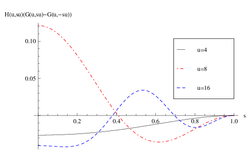
Refer to caption
Refer to caption
Figure 5: In sub-figure 5 we plot the integrand of equation (A.8), G⁡(u,s​u)​H​(u,s​u)G(u,su)H(u,su), for s∈(−1,1)s\in(-1,1). In sub-figure 5 we plot the integrand of equation (A.9), H⁡(u,s​u)​(G⁡(u,s​u)−G⁡(u,−s​u))H(u,su)\left(G(u,su)-G(u,-su)\right), for s∈(0,1)s\in(0,1). In both plots, the solid black line corresponds to u=4u=4, the dot-dashed red line corresponds to u=8u=8, and the dashed blue line corresponds to u=16u=16. Note that the integrand of equation (A.9) is well-behaved, whereas the integrand of equation (A.8) blows up at s=0s=0. For both plots, we chose the following parameters: t=1/2t=1/2, x=0x=0, μ=0.05\mu=0.05, σ2=0.34\sqrt{\sigma^{2}}=0.34, r=4r=4, V2=1V_{2}=1 and V3=1V_{3}=1.

References

  • [1] M. Al-Gwaiz, Sturm-Liouville theory and its applications, Springer Verlag, 2008.
  • [2] W. Amrein, A. Hinz, and D. Pearson, Sturm-Liouville theory: past and present, Birkhauser, 2005.
  • [3] F. Black and M. Scholes, The pricing of options and corporate liabilities, The Journal of Political Economy, 81 (1973), pp. 637–654.
  • [4] M. Bouzoubaa and A. Osseiran, Exotic Options and Hybrids: A Guide to Structuring, Pricing and Trading, Wiley, 2010.
  • [5] S.-Y. Choi, J.-P. Fouque, and J.-H. Kim, Option pricing under hybrid stochastic and local volatility, Submitted, (2010).
  • [6] J. Cox, Notes on option pricing I: Constant elasticity of diffusions, Unpublished draft, Stanford University, (1975). A revised version of the paper was published by the Journal of Portfolio Management in 1996.
  • [7] D. Davydov and V. Linetsky, Structuring, pricing and hedging double-barrier step options, Journal of Computational Finance, 5 (2001), pp. 55–88.
  • [8]  , Pricing options on scalar diffusions: An eigenfunction expansion approach, Operations Research, 51 (2003), pp. 185–209.
  • [9] J.-P. Fouque and M. J. Lorig, A fast mean-reverting correction to Heston’s stochastic volatility model, SIAM Journal on Financial Mathematics, 2 (2011), pp. 221–254.
  • [10] J.-P. Fouque, G. Papanicolaou, and R. Sircar, Derivatives in Financial Markets with Stochastic Volatility, Cambridge University Press, 2000.
  • [11] J.-P. Fouque, G. Papanicolaou, R. Sircar, and K. Solna, Short time-scale in S&P500 volatility, Computational Finance, 6 (2003).
  • [12]  , Singular perturbations in option pricing, SIAM J. Applied Mathematics, 63 (2003), pp. 1648–1665.
  • [13]  , Multiscale Stochastic Volatility for Equity, Interest-Rate and Credit Derivatives, Cambridge University Press, To Appear 2011.
  • [14] J.-P. Fouque, R. Sircar, and K. Sølna, Stochastic volatility effects on defaultable bonds, Applied Mathematical Finance, 13 (2006), pp. 215–244.
  • [15] J. Gatheral, The Volatility Surface: a Practitioner’s Guide, John Wiley and Sons, Inc., 2006.
  • [16] R. S. Goldstein and W. P. Keirstead, On the term structure of interest rates in the presence of reflecting and absorbing boundaries, SSRN eLibrary, (1997).
  • [17] P. Hagan, D. Kumar, A. Lesniewski, and D. Woodward, Managing smile risk.
  • [18] G. Hanson and A. Yakovlev, Operator theory for electromagnetics: an introduction, Springer Verlag, 2002.
  • [19] S. Heston, A closed-form solution for options with stochastic volatility with applications to bond and currency options, Rev. Financ. Stud., 6 (1993), pp. 327–343.
  • [20] E. Hillebrand, Overlaying time scales in financial volatility data, Advances in Econometrics, 20 (2006), pp. 153–178.
  • [21] D. Hinton and P. Schaefer, Spectral theory and computational methods of Sturm-Liouville problems, CRC, 1997.
  • [22] J. Hull and A. White, The pricing of options on assets with stochastic volatilities, The Journal of Finance, 42 (1987), pp. 281–300.
  • [23] A. Lewis, Applications of eigenfunction expansions in continuous-time finance, Mathematical Finance, 8 (1998), pp. 349–383.
  • [24]  , Option Valuation under Stochastic Volatility, Finance Press, 2000.
  • [25] V. Linetsky, Exotic spectra, Risk Magazine, (2002), pp. 85–89.
  • [26]  , The spectral decomposition of the option value, International Journal of Theoretical and Applied Finance, 7 (2004), pp. 337–384.
  • [27] R. Mendoza-Arriaga, P. Carr, and V. Linetsky, Time changed markov processes in unified credit-equity modeling, Mathematical Finance, 20 (2010), pp. 527–569.
  • [28] A. Mijatović, Local time and the pricing of time-dependent barrier options, Finance and Stochastics, 14 (2010), pp. 13–48.
  • [29] B. øksendal, Stochastic differential equations: an introduction with applications, Springer Verlag, 2003.
  • [30] A. Pelsser, Pricing double barrier options using laplace transforms, Finance and Stochastics, 4 (2000), pp. 95–104.
  • [31] I. Stakgold, Boundary value problems of mathematical physics, Society for Industrial Mathematics, 2000.
  • [32] E. Titchmarsh, Introduction to the theory of Fourier integrals, Clarendon Press Oxford, 1948.
  • [33] D. Zill and M. Cullen, Differential equations with boundary-value problems, Brooks/Cole Pub Co, 2008.
  • [34] D. Zwillinger, Handbook of differential equations, Academic Pr, 1998.