Black hole-neutron star mergers: effects of the orientation of the black hole spin
Abstract
The spin of black holes in black hole-neutron star (BHNS) binaries can have a strong influence on the merger dynamics and the postmerger state; a wide variety of spin magnitudes and orientations are expected to occur in nature. In this paper, we report the first simulations in full general relativity of BHNS mergers with misaligned black hole spin. We vary the spin magnitude from to for aligned cases, and we vary the misalignment angle from 0 to for . We restrict our study to 3:1 mass ratio systems and use a simple -law equation of state. We find that the misalignment angle has a strong effect on the mass of the postmerger accretion disk, but only for angles greater than . Although the disk mass varies significantly with spin magnitude and misalignment angle, we find that all disks have very similar lifetimes ms. Their thermal and rotational profiles are also very similar. For a misaligned merger, the disk is tilted with respect to the final black hole’s spin axis. This will cause the disk to precess, but on a time scale longer than the accretion time. In all cases, we find promising setups for gamma-ray burst production: the disks are hot, thick, and hyperaccreting, and a baryon-clear region exists above the black hole.
pacs
04.25.dg, 04.40.Dg, 04.30.-w, 47.75.+f, 95.30.SfI Introduction
Black hole-neutron star (BHNS) binary mergers present a remarkable opportunity to study strongly-curved spacetime and supernuclear-density matter in the most extreme, dynamical conditions. BHNS binaries in compact orbits emit strong gravitational waves, and they are expected to be one of the main sources for Advanced LIGO and VIRGO [1, 2]. Current estimates for the event rates of binary mergers coming from population synthesis models predict that Advanced LIGO will see about BHNS/yr, although uncertainties in the models allow for a large range of potential event rates, – 300 BHNS/yr [3]. These gravitational waves contain, in principle, a wealth of information on their source, such as the mass and spin of the black hole (BH) and the mass and radius of the neutron star (NS). Inferred properties of the NS could be used to constrain the NS equation of state. Information in the waves can only be extracted, however, by comparison with accurate numerically-generated predictions that provide the expected waveform for each possible BHNS system.
Mergers of BHNS binaries have also been proposed as potential progenitors of short-hard gamma-ray bursts (SGRB) [4]. The origin of SGRBs is not yet known, although it is certain that the engines are compact and located at cosmological distances, and there is evidence (such as their presence in nonstar forming regions) to support a mechanism different from that associated with long-soft GRBs, namely stellar core collapse. For BHNS mergers, the generation of a SGRB is possible only if the remnant black hole is surrounded by a massive, hot, thick accretion disk. Also, to obtain relativistic jets and a beamed outflow, a region mostly devoid of any matter is necessary (see e.g. [5] and references therein). Only numerical simulations in full general relativity with realistic microphysics can determine if these conditions are likely to be obtained.
Whether a disk forms or not will depend on the premerger characteristics of the binary, especially the BH mass, the NS radius, and the BH spin. Current estimates from population synthesis models suggest that most systems are likely to be formed with a black hole of . Relativistic simulations to date have considered cases of relatively low mass black holes ( ) [6, 7, 8, 9, 10, 11, 12, 13], for which the NS is expected to disrupt outside the innermost stable circular orbit (ISCO), making disk formation more likely. These simulations have found cases of massive disk formation, with resulting in the largest disks [12]. The NS radius is the parameter related to the equation of state that has the largest effect on the waveform and post-merger disk [13], with larger radii resulting in larger disks [8, 13].
The spin of the black hole can have a strong influence on the merger. The ISCO is smaller for prograde orbits around a spinning BH than for orbits around a nonspinning hole. Because disk formation is expected to be more likely if NS tidal disruption occurs outside the ISCO than if it occurs inside, BH spin can facilitate disk formation. With high BH spin, it is even plausible that BHNS binaries with the most likely mass ratios (7:1) give rise to substantial disks [14]. The magnitude of the BH spin is largely unconstrained by population synthesis models, as it comes mostly from the spin acquired during formation of the black hole in a core-collapse event [15]. The effect of aligned and antialigned spins was investigated in full general relativity for the 3:1 mass-ratio case by Etienne et al. [12]. They found that a large aligned spin (and correspondingly small ISCO) leads to a much more massive post-merger disk. For example, for and , a disk of can be obtained. For BHNS binaries with massive black holes (), forming a disk may in fact only be possible if the hole is spinning.
There is no reason to expect the black hole spin to be aligned with the orbital angular momentum. Population synthesis models predict a relatively wide distribution of orientations, with about half of the binaries having a misalignment between the BH spin and the orbital angular momentum of less than when the initial BH spin is [15]. Misalignment can reduce or reverse the BH spin effects described above. This can be understood by considering prograde orbits of test particles with small radial velocity, which become unstable farther away from the BH for inclined orbits than for equatorial orbits of the same angular momentum. Misalignment will also produce qualitatively new effects, including the precession of the premerger orbital plane and BH spin. The influence of misalignment has been studied for 10:1 mass-ratio binaries in the approximation that the spacetime is assumed to be Kerr. Rantsiou et al. [16] showed that, in this approximation, disks can be formed only at relatively low inclinations and only for near extremal black holes. Ultimately, though, simulations in full general relativity are needed to accurately model such systems.
In this paper, we report on fully relativistic studies of misaligned BHNS binaries. We limit ourselves to small mass systems () and a simplified equation of state, but we consider a significant range of black hole spin magnitudes and orientations. We confirm the results of Etienne et al [12] regarding the effects of an aligned BH spin. For misaligned spins, we find that the misalignment angle can have a strong effect on the post-merger disk mass, but only for angles greater than around . Although the disk mass varies greatly with BH spin, most other disk properties are very similar, including the accretion time scale, the location of the maximum density, the average temperature, and the entropy and angular momentum profiles. The disks are all thick, each with a height to radius ratio , nearly independent of . Crucially, they all have a baryon-clear region above and below the BH. The disks are misaligned with the final BH spin by . They do precess about the BH spin axis, but without reaching a fixed precession rate. Indeed, the steady-state precession time scale is expected to be significantly longer than the accretion time scale.
This paper is organized as follows. In Sec. II, we discuss the method used to construct the very general BHNS initial data we use. We also discuss in detail the improvements to our evolution code that have increased the accuracy by an order of magnitude over the results presented in Duez et al. [11]. We then present our run diagnostics in Sec. III. The different cases to be evolved are described in Sec. IV. We then present the results of the simulations in Secs. V and VI. Finally, we draw conclusions in Sec. VII.
II Numerical methods
II.1 Initial data
For numerical evolutions of Einstein’s equations, we decompose the spacetime under study into a foliation of spacelike hypersurfaces parametrized by the coordinate . Einstein’s equations can be written in the form of hyperbolic evolution equations plus a set of constraints that have to be satisfied on each slice. Our initial data at must be chosen such that it satisfies these constraints. We construct initial data using the Extended Conformal Thin Sandwich formalism (XCTS) [17, 18]. If we write the spacetime metric as
| (1) | |||||
the initial data to be determined include the lapse , the shift vector , the conformal factor , the conformal 3-metric and the extrinsic curvature (where is the Lie derivative along the normal to the slice). The constraints can be expressed as a set of 5 coupled elliptic equations for the lapse, shift, and conformal factor [18]. The physical properties of the system are then determined by the choice of the remaining free parameters: the trace of the extrinsic curvature , the conformal metric , their time derivatives and , and the matter stress-energy tensor .
The system of elliptic equations is solved using the spectral elliptic solver spells developed by the Cornell-Caltech collaboration [19], and initially used to construct initial data for binary black hole systems by Pfeiffer et al. [20, 18]. A detailed presentation of the methods used for the construction of BHNS initial data was given in Foucart et al. [21]. Here, we limit ourselves to a brief summary plus a description of the changes made to accommodate the possibility of arbitrary spin orientation.
As the system is expected to be initially in a quasiequilibrium state, with the binary in a low-eccentricity circular orbit of slowly decreasing radius, we work in a frame comoving with the binary and set the time derivatives to zero: and . As for and , we make a choice inspired by the results of Lovelace et al. [22] for binary black hole systems. Close to the BH, the metric matches its Kerr-Schild values for a BH of the desired mass and spin, while away from the BH, the conformal metric is flat and . The transition between these two regions is done by using the following prescription:
| (2) | |||||
| (3) | |||||
| (4) | |||||
| (5) |
where the subscript refers to the Kerr-Schild values, () is the coordinate distance to the center of the BH (NS), the coordinate radius of the BH apparent horizon, is the dimensionless spin of the BH, a constant of the order of the mass ratio, the coordinate location of the BH center with respect to the center of mass of the system, and is some freely specifiable width, chosen so that the metric is nearly flat at the location of the NS. The parameter , which is designed to impose a flat background at the location of the NS, is set to for .
Boundary conditions are imposed at infinity and on the apparent horizon of the BH (since the inside of the BH is excised from our computational domain). The boundary conditions at infinity are chosen so that the metric is asymptotically flat, while the inner boundary conditions follow the prescriptions of Cook and Pfeiffer [23], which make the inner boundary an apparent horizon in quasiequilibrium. There is some freedom in these boundary conditions: on the apparent horizon, the conformal lapse is not fixed (we set it to the value of an isolated Kerr BH), and the shift is determined only up to a rotation term . The value of determines the spin of the BH, but the exact relation between and the spin is unknown a priori; to get the desired BH spin, we have to solve iteratively for . On the outer boundary, the shift can be written as
| (6) |
where allows for a global rotation of the coordinates, for a radial infall with velocity , and for a boost. As an initial guess for the orbit of the binary, we can set the radial velocity at to 0 (). This assumption, as well as the quasiequilibirum formalism, clearly neglects the evolution of the orbit over time through the radial infall of the binary and the precession of the orbital plane. Both effects are, however, acting over relatively long time scales: over its first orbit, even the binary with the most inclined spin considered here (s.5i80 in the later sections) goes through less than of a full precession period of the BH spin while the coordinate separation between the compact objects is reduced by about . One known effect of the quasi-circular approximation is that the binary will have a nonzero eccentricity. The eccentricity can be decreased by modifying the initial values of and [24] (see also [21] for an application of that method to BHNS binaries) as long as the initial eccentricity and orbital phase can be accurately measured. Here, we only apply this technique when the spin of the BH is aligned with the orbital angular momentum of the binary. For precessing binaries, significantly reducing the eccentricity would require a larger initial separation for which the effects of eccentricity, precession and radial infall can be properly disantangled.
In the presence of matter, additional choices are required. We assume that the fluid is in hydrostatic equilibrium in the comoving frame, and require that its 3-velocity is irrotational. The first condition gives an algebraic relation between the enthalpy of the fluid, its 3-velocity , and the metric , while the second leads to another elliptic equation determining the velocity field. These equations are coupled to the constraints: the whole system can only be solved through an iterative method. For a BH with a spin aligned with the total angular momentum of the system, that method is described in Foucart et al. [21]: we solve for the metric using spells, then determine the new value of the enthalpy , as well as the orbital angular velocity (chosen so that the binary is in quasicircular orbit), the position of the BH in the equatorial plane (so that the total linear momentum vanishes), and the free parameter (to drive the spin of the BH to its desired value). Finally, we solve for the velocity field through the elliptic equation imposing an irrotational configuration, and go back to the first step.
In order to construct initial data for BHs with a spin that is not aligned with the orbital angular momentum of the binary, a few changes are necessary. First, we do not assume that is aligned with the orbital angular momentum. Instead, all 3 components of are solved for. We also abandon the assumption of equatorial symmetry, and control the position of the BH along the -axis of the orbital angular momentum by requiring that the NS is initially moving in the -plane, with its center in the plane (the coordinate of the location of the BH is chosen so that the condition is satisfied at the center of the NS). Finally, to guarantee that we impart a boost to the whole system through the boundary condition at infinity: . The center of mass is then expected to have a global motion during inspiral corresponding to that boost, and we check in Fig. 1 that this is indeed the case. By adding these conditions to the iterative procedure used to generate BHNS initial data, we are able to obtain high-precision initial configurations for arbitrary values of the orientation of the BH spin.

II.2 Evolution
The simulations presented here use the SpEC code developed by the Cornell-Caltech-CITA Collaboration [25]. To evolve BHNS systems, the two-grid method described in Duez et al. [11] is used. Einstein’s equations are evolved on a pseudospectral grid, using the first-order generalized harmonic formulation [26], while the hydrodynamical equations are solved on a separate finite difference grid called the “fluid grid”. The hydrodynamic equations are written in conservative form
| (7) |
To compute the flux on the faces of each finite difference cell, we use the third-order shock capturing PPM reconstruction method [27]. More details on the numerical methods used can be found in Duez et al. [11]. However, since the publication of [11], several important improvements have been made to the code, which are described in the following subsections.
II.2.1 Dynamic regridding
To accurately evolve a BHNS binary while determining its gravitational wave emission, simulations have to resolve events occurring at very different scales. When the neutron star is disrupted and a disk forms, we expect shocks in the disk, and steep density and temperature gradients close to the BH. But the disruption of the star also leads to the creation of a long tidal tail which can initially contain up to of the initial mass of the star and expand hundreds of kilometers away from the center of the BH [13]. Clearly, both the sharp, small-scale features around the black hole and the large-scale tidal tail should be properly resolved if we want to follow the formation of an accretion disk. Furthermore, to extract gravitational waves accurately, the evolution of the gravitational fields should extend to the wave zone, in regions where no matter at all is present.
Because we use different grids to evolve the metric and the fluid variables, the spectral grid on which we solve the generalized harmonic equations can be extended into the wave zone while the fluid grid used for the relativistic hydrodynamical equations only covers the region where matter is present. Our earlier simulations [11] were limited to nonspinning black holes. In that case, most of the matter was rapidly accreted onto the hole and the tidal tails and accretion disks were small enough that manually expanding the fluid grid at a few chosen timesteps allowed us to resolve the evolution of the fluid at a reasonable computational cost. For spinning black holes, this is no longer the case: cost-efficient evolutions require a grid with points concentrated in the high-density regions close to the BH, and coarser resolution in the tail. Furthermore, as the evolution of the fluid is highly dynamical, interrupting the simulation whenever the finite difference grid is no longer adapted to the fluid configuration becomes impractical. One solution would be to use an adaptive mesh refinement scheme, similar to the codes used by Yamamoto et al. [28] and Etienne et al. [12]. In our code, we choose instead to use a map between the fluid grid and the pseudospectral grid that concentrates grid points in the region close to the black hole and automatically follows the evolution of the fluid.
To do this, we measure the outflow of matter across surfaces close to but inside of the fluid grid boundaries. As soon as the outflow across one of these surfaces crosses a given threshold (chosen so that the amount of matter leaving the grid over the whole simulation is negligible compared to the final mass of the accretion disk), the grid expands. The opposite is done on fixed surfaces farther away from the grid boundaries to force the grid to contract whenever the fluid is moving away from a boundary. The map itself is the combination of:
- (i)
A translation of the center of the grid, to follow the general motion of the fluid
- (ii)
A linear scaling of each coordinate axis, to adapt to its expansions and contractions
- (iii)
A radial map smoothly transitioning from a high resolution region close to the black hole to a lower resolution region far away from it. The exact form of the map is
(8) (9) where the coefficients are chosen so that the map is at and and is chosen so that the grid is of the desired size. The radii and are fixed for the whole evolution and will determine respectively the minimum resolution in the neighborhood of the black hole and the characteristic lengthscale of the transition between the high and low resolution regions.
II.2.2 Excision
We find that our hydrodynamics code is more stable near the excision zone if we switch from PPM to the more diffusive MC reconstruction [29] in the vicinity of the excision zone. Therefore, we replace the face values determined by PPM reconstruction, with a weighted average:
| (10) |
where for and for .
The MC face-value computation must be altered when its regular stencil
would extend into the excised region, and doing this properly turns out to
be important for stability. Consider a one-dimensional problem with
grid points . Then the face-value reconstruction of
the function from the left and
from the right must be adjusted as follows.
(i) If is in the excision zone, but is outside,
set and
(ii) If is in the excision zone, but is outside,
set and
(iii) If is outside the excision zone, but is inside,
set
(iv) If is outside the excision zone, but is inside,
set
We also observed that the stability of our code close to the excision surface was strongly affected by the details of the interpolation method chosen for the communication from finite difference to spectral grid in that region. Previously, the interpolation stencil was shifted away from the excision boundary until the entire stencil was out of the excision zone. This could lead to unstable evolutions or large interpolation errors if the excision region happened to be located close to the boundary between two subdomains of the finite difference grid, and acceptable stencils could only be found far from the point we were interpolating to — or could not be found at all (to limit MPI communications, the stencil has to be entirely contained in one subdomain). Currently, we limit the displacement of the stencil to a maximum of 3 grid point separations. If there is no good stencil within that distance, we decrease the order of the interpolation, and keep doing so until an acceptable stencil is found.
Another interpolation method would be to forbid any displacement of the stencil, and immediately drop to lower order as soon as part of the stencil lies within the excision zone. Both algorithms are equally robust, but when tested on an actual BHNS merger the first appeared to perform better at maintaining a smooth solution and low constraint violations on the excision surface. Accordingly, we chose it as our standard interpolation method and used it for all simulations presented in this paper.
II.2.3 Coordinate evolution
In the generalized harmonic formulation, the evolution of the inertial coordinates is given by the inhomogeneous wave equation
| (11) |
where is the covariant derivative along . The evolution of the function can be freely specified, but its value on the initial slice is determined by the initial data (the lapse and shift at fix the initial evolution of the gauge). While the binary spirals in, we choose in the coordinate frame comoving with the system. In our previous paper [11], we changed the gauge evolution during the merger phase by damping exponentially in the comoving frame:
| (12) |
where is the disruption time—the time at which we begin damping— and is a damping time scale of order 10 ( being the total mass of the system). Further experimentation has shown that it is better not to change near the excision zone. In our current simulations, we set
| (13) | |||||
| (14) |
during the merger phase, where is the distance to the center of the black hole in the comoving frame, and is the excision radius.
II.2.4 Evolutions with fixed metric
During the merger of a BHNS binary, both the spacetime metric and the fluid configuration are highly dynamical. Einstein’s equations have to be solved together with the conservative hydrodynamics equations, and the evolution of that coupled system is computationally intensive. However, a few milliseconds after merger, the BH remnant settles into a quasistationary state as it accretes slowly from the surrounding accretion disk. Then, the evolution of the metric does not have a strong influence on the behavior of the system. In numerical simulations, we can thus extract some information on the long-term behavior of the final black hole-accretion disk system by neglecting the evolution of the metric and only evolving the fluid (c.f. [30]). Using this approximation, our code runs about 4 times faster.
To test the limitations of this method, we evolve the coupled system past the time at which we begin the approximate, fluid-only evolution. We look for differences in the accretion rate or the characteristics of the disk (temperature, density, inclination) between the two methods used. As long as we wait for the properties of the black hole to settle down before switching to the approximate evolution scheme, the two methods show extremely good agreement — except for the highest spin configuration, which leads to a massive disk that cannot be evolved accurately by fixing the background metric. In Fig. 2 we show the evolution of the density profile of a disk using both the full GR evolution and the fixed-metric approximation. The evolution of the accretion disk is mostly unaffected by the change of evolution scheme.

III Diagnostics
An indispensable test of numerical accuracy is convergence with grid resolution. We have evolved most of the cases discussed below at three resolutions. We call these Res1, Res2, and Res3; they correspond to , , and gridpoints, respectively, on the fluid grid and to , , and collocation points on the pseudospectral grid.
The black hole is described by its irreducible mass , its spin , and its Christodoulou mass . The spin is computed using the approximate Killing vector method [22].
To monitor the nuclear matter, we first measure the baryonic mass on the grid as a function of time. Initially, this will be the baryonic mass of the neutron star. After the tidal destruction of the star, it will be the sum of the accretion disk and the tidal tail masses. At late times (more than 10ms after merger), it will be the baryonic mass of the disk. The accretion time scale is .
We also analyze the heating in the disk. This is done through both an entropy and a temperature variable. When evolving with microphysical equations of state, the temperature and entropy are provided directly. For this study, we use a -law equation of state, so we need a way to estimate the entropy and temperature. The entropy measure we define as , where is the polytropic constant obtained from the relation between the pressure and the baryon density (), and is its initial, cold value. To estimate the physical temperature, , we assume that the thermal contribution to the specific internal energy is given by a sum of ideal gas and blackbody components:
| (15) |
where is the nucleon mass, and the factor reflects the number of relativistic particles, and is itself a function of . (See [8, 12], who also make this assumption.) For the most part, we will report density-averaged values of and . For example, the density-averaged entropy is
| (16) |
To launch a GRB, a baryon-clean region above the disk is probably needed. This does not mean that a wider clean region is always better, since a thick disk can help collimate the outflowing jet — but we want to determine whether such a region exists or not. To estimate the baryon-poor opening above our disks, we define the opening angle . This angle specifies the widest cone oriented along the BH spin in which the condition is everywhere satisfied: if is the opening angle within which we have at radius and azimuthal coordinate , then . In these simulations, the numerical method requires atmospheric corrections to be applied starting at , so that it is impossible to reliably predict the behavior of matter below that threshold. Therefore, we set .
For precessing binaries we also compute the tilt and twist of the disk, as defined by Fragile & Anninos [31]. If are the inertial coordinates, the stress-energy tensor, the Levi-Cevita tensor (with its last index limited to nonzero values), the angular momentum of the BH and an arbitrary unit vector orthogonal to , then , and the disk angular momentum are given by
| (17) | |||||
| (18) | |||||
| (19) | |||||
| (20) | |||||
| (21) |
These parameters determine the inclination and the precession of the disk with respect to the spin of the black hole: if , then the orbital angular momentum of the disk at radius is written as
| (22) |
Another useful property of the disk is its scale height, . For a disk with exponentially decreasing density, is defined by . Here, however, the vertical profile of the disk is significantly more complex, and various definitions of could be considered. We use the spread of the density distribution on a sphere of constant radius with its polar axis along and define
| (23) |
The parameter is somewhat arbitrary. For an exponential profile , while for a constant density profile ( for and otherwise) we have . The disks observed in our simulations are somewhat in between these two extremes. Accordingly, we make the approximate choice .
To measure the accuracy of our simulations, we monitor the ADM Hamiltonian and momentum constraints, and the generalized harmonic constraints [26]. At our middle resolution, peaks below for all cases and is less than during most of the inspiral. We also monitor the ADM mass and angular momentum . An important check of our simulations is that the changes in these quantities match the flux of energy and angular momentum in the outgoing gravitational radiation, which we reconstruct from the Newman-Penrose scalar as in Ref. [32].
IV Cases
In order to assess the influence of the black hole spin on the disruption and merger of BHNS binaries, we study configurations for which all other physical parameters are held constant. The mass of the black hole is , where is the ADM mass of an isolated neutron star with the same baryon mass as the star under consideration, and the initial coordinate separation is , with . For the nuclear equation of state, we use the polytrope
| (24) |
where is a fluid variable related to, but not equal to, the physical temperature. We set and choose so that the compaction of the star is . For polytropic equations of state, the total mass of the system does not have to be fixed: results can easily be rescaled by (see e.g. Sec. II-F of Foucart et al. [21]). However, whenever we choose to interpret our results in physical units (ms, km, ), we will assume that (). For that choice, the neutron star has a radius , and the initial separation is .
The different initial configurations and black hole spins studied are summarized in Table 1. We consider 3 different magnitudes of the dimensionless spin , all aligned with the orbital angular momentum. Then, we vary the inclination angle between the spin of the black hole and the initial angular velocity of the system, . Considering that most BHNS binary systems are expected to have (Belczynski et al. [15]), with about half of the binaries at , we choose . The orientation of the component of the BH spin lying in the orbital plane could also have measurable consequences. For example, Campanelli et al. [33] showed that the superkick configuration found in binary black hole systems is sensitive to the direction of the misaligned component of the BH spin. For BHNS binaries, kicks are relatively small, and we are more interested in the characteristics of the final black hole-disk system. After looking at different orientations for , we find that the influence of the orientation of the misaligned component of the BH spin is negligible compared to the influence of . For this first study of misaligned spins, we will thus limit ourselves to configurations for which the initial spin lies in the plane generated by the initial orbital angular momentum and the line connecting the two compact objects. As the different initial configurations do not use the same background metric, there is no guarantee that two binaries with the same initial coordinate separation can be directly compared. A better comparison between initial configurations is the orbital angular velocity of the system. In Table 1, we show that all configurations have initial angular velocity within of each other. This is the level of error that we expect from the quasiequilibrium method for binaries at this separation.
| Case | ||||||
|---|---|---|---|---|---|---|
| s0 | 0 | - | 4.16e-2 | 9.5e-3 | 0.66 | 7.5ms |
| s.5i0 | 0.5 | 0 | 4.11e-2 | 1.01e-2 | 0.91 | 11.4ms |
| s.9i0 | 0.9 | 0 | 4.13e-2 | 9.6e-3 | 1.13 | 15.0ms |
| s.5i20 | 0.5 | 20 | 4.09e-2 | 1.01e-2 | 0.90 | 10.5ms |
| s.5i40 | 0.5 | 40 | 4.10e-2 | 1.01e-2 | 0.87 | 9.9ms |
| s.5i60 | 0.5 | 60 | 4.11e-2 | 9.9e-3 | 0.82 | 9.0ms |
| s.5i80 | 0.5 | 80 | 4.13e-2 | 9.6e-3 | 0.76 | 7.7ms |
V The nonspinning case: a test of our accuracy
As an example, we consider the case s0, in which the BH is initially nonspinning. We evolve this case at each of our three resolutions. After a short (two orbits) inspiral, the neutron star is disrupted, and most of the matter is quickly swallowed by the black hole. The remainder expands into a tidal tail and then falls back to form an accretion disk.
Nearly identical systems have been studied both by Shibata et al [9] and by Etienne et al [12]. The former found an insignificant disk after merger, while the latter found 4% of the NS mass still outside the hole 300 () after merger. Both groups found a final BH spin of . We find a disk mass of 3.7% at 300 after merger, smaller than in [12], but closer to this result than to that in [9]. Our final BH spin is 0.56, in agreement with both previous studies.
In Fig. 3, we show the evolution of and for the entire merger phase for the three resolutions. Reassuringly, the different resolutions give very similar results, with the two higher resolutions being closest together. The baryonic mass is initially constant before accretion starts. Then, as the NS is disrupted and the core of the star is swallowed, drops rapidly. It next levels off while the remaining matter is in an accretion disk and an expanding tidal tail. When the tidal tail falls back onto the disk, there is a second phase of rapid accretion, after which the accretion rate settles down to a low value. At the end of the simulation, the accretion time scale is , implying that the total lifetime of the disk would be around 75ms. At late times, the deviation in between resolutions becomes somewhat larger, indicating that our errors have accumulated to about of the initial mass. For the purposes of this paper, this is adequate, since the disk on these time scales is affected by magnetic and radiation processes not included in the simulations. However, future long-term disk simulations will require higher accuracy.
As for the entropy, at the beginning of the merger it only deviates from zero because of numerical heating during the inspiral. As expected, this numerical heating is significantly lower at higher resolutions. The post-merger heating is not numerical, but a physical consequence of shocks in the disk and the disk-tail interface. A confirmation that the heating is physical is that it is nearly the same for all resolutions, and its magnitude is much larger than the numerical heating. When the disk settles, there is no further shock heating, so the entropy levels off. This indicates that the heating due to numerical viscosity is small compared to shock heating. Unfortunately, this is not the same as saying that the numerical viscosity is irrelevant altogether. However, the closeness of at each resolution indicates that this viscosity is not the main driving force of the accretion. The average temperature behaves in a way similar to the entropy. Starting from low values, it increases after the merger and stabilizes around 3MeV. All resolutions show the same growth, and all level off at the same value. After leveling off, though, displays 0.1MeV oscillations that do not converge well, another indication that our accuracy is sufficient for some but not all purposes.

In Fig. 4, we plot the ADM energy and orbital-axis angular momentum measured on a surface from the center of mass of the system. Also plotted is the evolution of these quantities expected from the gravitational radiation through this surface. Overall, the agreement is quite good, although there is some deviation in a while after the merger. This seems to be associated with an increase in constraint violations at the merger time. The relative constraint violations, as measured by , peak slightly below 1% at the middle resolution. The corresponding values for the ADM constraints are 1 –2 %, before both constraints fall back to low values. The deviations in happen around the time this constraint-violating pulse reaches the surface.

We have checked several other quantities, including the black hole mass and spin and the gravitational waveform. All of these show very good convergence.
VI Results
The general behavior of our simulations is typical of BHNS binaries for which the NS is disrupted outside the innermost stable circular orbit of the BH. From an initial separation of , the compact objects go through 2-3 orbits of inspiral driven by the emission of gravitational waves. When the distance between them has been reduced to about , tidal forces cause the neutron star to disrupt. Most of the matter is rapidly accreted into the black hole, while the rest is divided between a long tidal tail, expanding about away from the black hole, and a developing accretion disk. The duration of the inspiral varies with the spin of the BH, with the component of the BH spin along the orbital angular momentum delaying the merger. The merger time , which we define as the time at which 50% of the matter has been accreted onto the BH, is listed for all cases in Table 1.
The resulting accretion disk is highly asymmetric, and evolves in time. When the disk first forms, around 5ms after merger, it creates a torus of matter with its peak surface density (baryon density integrated over the height of the disk) at and a temperature . Then, as matter accretes from the tidal tail and shocks heat the fluid, the disk expands quickly. About after merger, the disk starts to settle into a stable, slowly accreting state. To compare the different configurations studied here, we look at the properties of this late-time stable configuration, listed in Table 2. In Table 3, we give the characteristics of the final black hole, as well as the kick velocity, the energy content of the emitted gravitational waves, and the peak amplitude of a dominant (2,2) mode of the waves. [The (2,2) and (2,-2) are the strongest modes, with nearly equal amplitude. See Section VI.2 on the higher modes.]
| Case | |||||||
|---|---|---|---|---|---|---|---|
| s0 | 5.2% | 3.0MeV | 50km | 0.20 | |||
| s.5i0 | 15.5% | 3.5MeV | 50km | 0.25 | |||
| s.9i0 | 38.9% | 5.6 MeV | 20km | 0.18 | |||
| s.5i20 | 14.5% | 3.6MeV | 50km | 0.20 | |||
| s.5i40 | 11.5% | 3.8 MeV | 50km | 0.22 | |||
| s.5i60 | 8.0% | 3.7MeV | 50km | 0.20 | |||
| s.5i80 | 6.1% | 3.6MeV | 50km | 0.25 |
| Case | ||||||
|---|---|---|---|---|---|---|
| s0 | 0.97 | 0.56 | 53 | 0.98% | 0.020 | |
| s.5i0 | 0.94 | 0.77 | 60 | 0.92% | 0.012 | |
| s.9i0 | 0.89 | 0.93 | 52 | 0.95% | 0.009 | |
| s.5i20 | 0.95 | 0.76 | 60 | 0.89% | 0.012 | |
| s.5i40 | 0.96 | 0.74 | 61 | 0.91% | 0.013 | |
| s.5i60 | 0.96 | 0.71 | 54 | 0.95% | 0.014 | |
| s.5i80 | 0.97 | 0.66 | 67 | 0.95% | 0.017 |
VI.1 Effects of spin magnitude
To test the effects of BH spin magnitude, we compare our results for s0, s.5i0, and s.9i0. A comparison of this type has already been performed by Etienne et al [12]. Our cases are different, though: unlike them, we do not consider an antialigned case, but we do push the BH spin to a slightly higher level in our run s.9i0.
Run s.9i0 presented special numerical challenges. In spec, the singularity and inner horizon of the BH have to be excised from the numerical grid while the apparent horizon must remain outside the excision surface. But for nearly extremal black holes the region between the inner horizon and the apparent horizon becomes very narrow. To perform excision in such cases, the excision boundary must nearly conform to the apparent horizon. We do this by introducing a coordinate map in the initial data so that the horizon is initially spherical on the pseudospectral grid. We then use our dual frame coordinate-control method [34] to fix the location of the horizon throughout the whole simulation. For lower spins this is not necessary, and we only begin to control the horizon location at the time of neutron star disruption. That modification excepted, case s.9i0 was simulated in exactly the same way as the other cases. The deviation between the results at resolutions Res2 and Res3 is somewhat larger than in the other cases (though still quite small). To be more exact, the relative deviation in the disk mass between Lev2 and Lev3 is about 9% (3% of the NS mass) for s.9i0 while it was about 5% for s0, and the deviation in merger time is about 4% for s.9i0 but only 0.3% for s0. The difference indicates that high resolution is needed when studying such extreme cases.
We find that systems with higher spiral in more slowly: from the same initial separation, s0, s.5i0, and s.9i0 take roughly 2, 3, and 3.7 orbits, respectively, before NS disruption begins. This effect exists in the post-Newtonian treatment [35] and it has already been seen both in binary black hole (e.g. [36]) and BHNS [12] simulations. Because of the prolonged inspiral for the high-spin cases, more angular momentum is radiated: 0.11 for s0 vs 0.14 for s.9i0. Additionally, as the BH becomes nearly extremal, increasing the spin becomes more and more difficult. This is reflected in the final spin of the BH: while increases from 0 to 0.56 for s0, it only increases from 0.9 to 0.93 for s.9i0.
We also confirm that the post-merger accretion disk mass increases significantly as the magnitude of the aligned BH spin is increased, as shown in Fig. 5. This is in qualitative agreement with Etienne et al. About (11ms) after merger they find 20% for an system, while for our system, we find 35% at a similar time.

VI.2 Effects of spin orientation
Most BHNS binaries are expected to have at least a moderate misalignment between the spin of the BH and the total angular momentum [15], and this should affect all stages of the binary evolution.
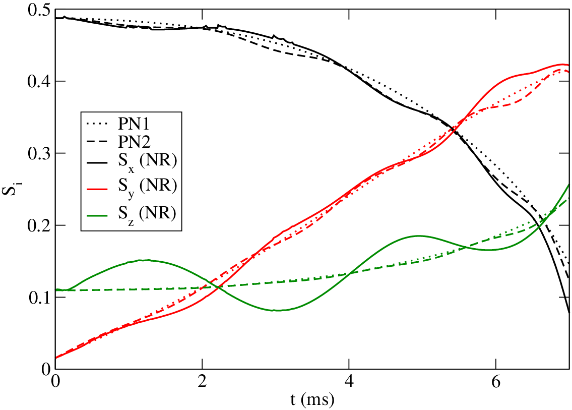
During inspiral, the orbital angular momentum and the BH spin precess around the total angular momentum of the system. The evolution of the coordinate components of the BH spin for the s.5i80 case is shown in Fig. 6. Over the two orbits of inspiral, the spin goes through about a quarter of a precession period. The qualitative evolution of the spin is well described by post-Newtonian corrections (see e.g. [37]), even though our simulation uses a different gauge choice. As for aligned spin, the infall velocity varies between cases: the larger the component of the spin aligned with the angular momentum, the slower the inspiral. Not too surprisingly, we find a monotonic decrease of the merger time with increasing misalignment angle , with for .
 |
 |
 |
 |
The disruption of the star and formation of a disk, shown in Fig. 7, proceed somewhat differently from what is observed for nonprecessing binaries. As before, the disruption of the star is accompanied by the formation of a long tidal tail. But because of the inclination of the BH spin, the orbital plane of the fluid continues to precess after disruption. Because the precession rate varies with the distance to the hole, the tail and the disk do not remain in the same plane. While for nonprecessing binaries matter from the tail falls back within the orbital plane of the disk, here matter is added to the disk at an angle varying in time. This significantly modifies the nature of the tail-disk interactions. At small inclination angles (), we have a direct collision between the developing disk and the tidal tail, while for larger inclinations the disk is initially formed of layers of high-density material at different angles with respect to the black hole spin.
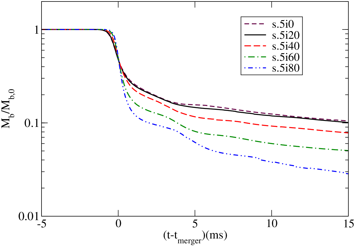
The mass of the disk, plotted in Fig. 8, decreases as the inclination of the binary increases. The transition between low and high mass disks is continuous, but more rapid at large inclinations: for , of the initial mass of the star () remains either in the tail or in the disk 5ms after merger. This is roughly similar to the disk formed for . At higher inclinations, the size of the disk drops sharply, to about of the initial mass of the star. We expect the disk mass to be even lower for antialigned spins (), though such configurations appear less likely to be found in astrophysical systems. These changes in the disk mass with the orientation of the BH spin show some similarities with the results of Rantsiou et al. [16], obtained in the small mass-ratio limit () by using a static background metric. They found that for a disk to be formed, the condition has to be satisfied. As our simulations use a mass ratio , which is more favorable to the formation of a disk, it is not too surprising that even high inclinations leave us with a significant disk; however, the influence of inclination remains important for . These factors are particularly useful when considering the potential of the final remnant to be a short gamma-ray burst progenitor. Since the influence of a misaligned BH spin is only felt for , the majority of BHNS binaries can form disks about as massive as is predicted by simulations that do not take into account the inclination of the BH spin.
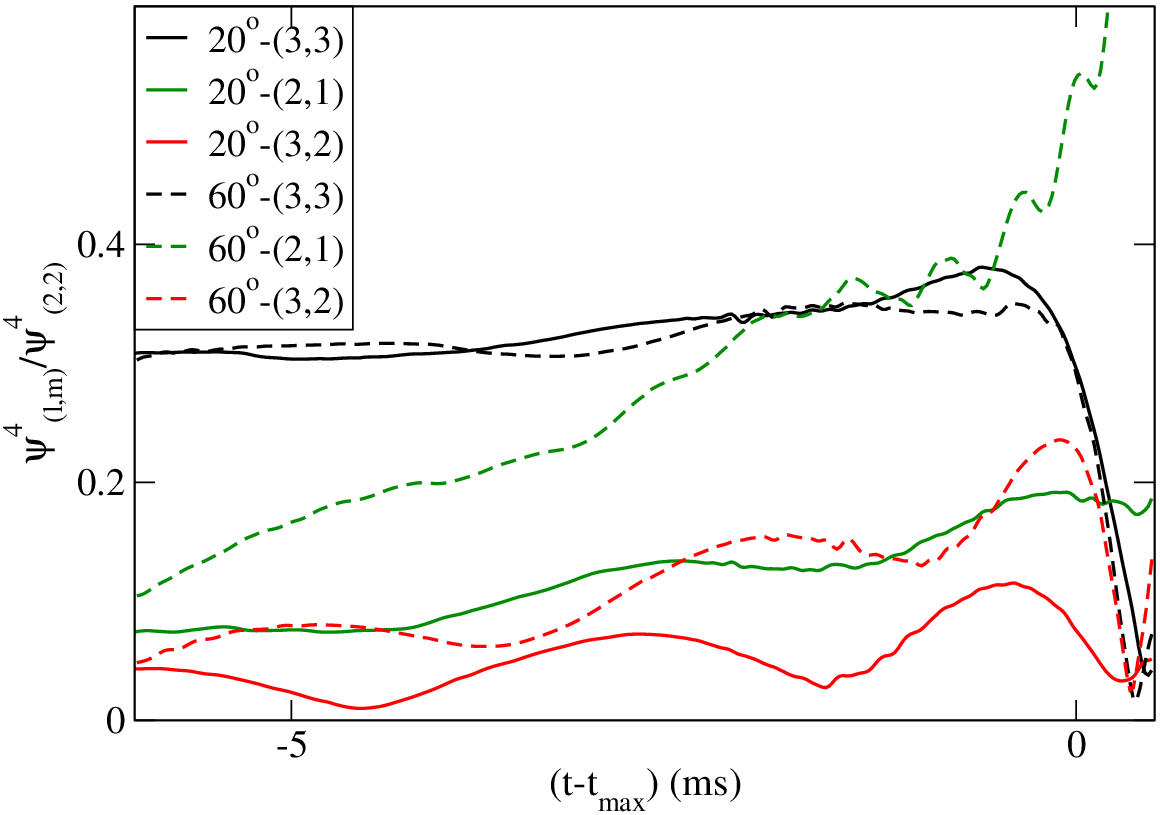
The gravitational wave signal is also significantly affected by the value of . We expand the Newman-Penrose scalar extracted at using the spin-weighted spherical harmonics and choosing the polar axis along the initial orbital angular momentum of the binary. The peak amplitude of the dominant (2,2) mode of will increase for large inclinations, as could be expected from the results obtained for aligned spins; here too, a large component of the spin along the orbital angular momentum works against large amplitudes. Additionally, the contribution of subdominant modes can become significant at large inclinations. In Fig. 9, we show the ratio of the amplitude of the scalar to the amplitude of the (2,2) mode for various modes and for . The modes most strongly affected by the precession of the binary are the (2,1) and (3,2) modes, the first reaching half the amplitude of the dominant mode around merger for the s.5i60 simulation. Analytical predictions for the effect of a precessing trajectory on the modal decomposition of the gravitational wave signal have been derived by Arun et al. [39]. We find qualitative agreement with their results if we assume that the compact objects follow the trajectories obtained from our numerical simulations. In particular, we note that for precessing binaries, the frequency of the (2,1) mode is closer to than to . The (2,1) and (2,2) modes have similar frequencies, so that the ratio of their amplitude computed using the scalar is close to the result one would obtain by using the gravitational strain instead. This will not be true for the (3,3) mode, which has a frequency : since , we have .
In Fig. 10, we plot the gravitational strain as observed from a distance of for the simulations s.5i0 and s.5i80. The three waveforms correspond to observation points whose lines of sight are inclined by , and with respect to the initial orbital angular momentum of the system. Over the short inspiral considered here, the effects of precession are relatively small. The main difference visible in these waveforms is the slower inspiral experienced by the binary with aligned spin. We can also note that in the misaligned configuration the star does not disrupt as strongly as in the aligned case, causing the cutoff of the wave emission to occur at a later time. As a consequence, the cutoff frequency of the wave is larger for misaligned spins than for aligned spins. This explains why the amplitude of the gravitational strain is comparable for both configurations, while the misaligned case showed a significantly larger amplitude when the wave was measured using the scalar (a similar effect occurs if both spins are aligned but of different magnitudes). Finally, the precession of the orbit causes the gravitational wave emission of the misaligned configuration to peak at a non-zero inclination with respect to the initial orbital angular momentum. Here, at the time of merger the wave measured at an inclination of is slightly larger than at . For these effects to be more visible, and in particular for a full precession period to be observable, longer simulations are required ( orbits).

VI.3 Post-merger accretion disks
The evolution of the accretion disk over time scales comparable to its expected lifetime is likely to be significantly influenced by physical effects that are not taken into account in our simulations, mostly the magnetic effects and the impact of neutrino cooling. We do not expect the results of our simulations to accurately represent the details of the late-time evolution of the disk, but we can nonetheless extract some information regarding the general characteristics of the final remnant. To obtain these approximate results, which are summarized in Table 2, we use the fixed-metric approximation described in Sec. II.2.4, starting after merger. At that time, the disk is still expanding, and will typically settle down to a more stable quasiequilibrium profile with a relatively low accretion rate over about .
The coordinate distance between the peak surface density of the disk (averaged over all points at a given coordinate radius) and the center of the BH shows no strong or monotonic dependence on the BH spin. After the initial expansion of the disk, variations in the details of the interactions between the tidal tail and the accretion disk can lead to different evolutions of the density profile. On average, the disks tend to expand slightly, while their density decreases because of continued accretion onto the black hole. However, neither the tidal tail nor the disk are homogeneous, so that the evolution of the density profile shows significant oscillations around that average behavior. The accretion rate is larger for the more massive disks, so that the expected lifetime of the disk is of the same order of magnitude for a nonspinning BH () as for the highly spinning BH ().
The thermal evolution of the disk does not vary much between configurations. The temperature rises rapidly during the formation of the disk, then stabilizes at about 3.5MeV in each case — although the average entropy is about 10% lower for spinning black holes than for s0. For most configurations, the temperature then remains relatively stable for the rest of the evolution, with oscillations of order 10%. The highest spin configuration s.9, however, reaches significantly higher temperatures, with . Fig. 11 shows the entropy and specific angular momentum profile of three of our disks at the end of the simulation. At the final time, each of the disks shows an inverted entropy gradient in the inner region between the black hole and the radius of maximum surface density. The entropy difference between the inner edge of the disk and the density maximum is about 10%. However, the disk is at least partially stabilized by the strong shear in the rotational velocity in these inner regions.
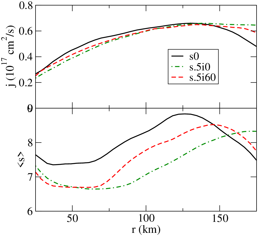
Lower panel: For the same configurations, entropy of the disk averaged over all points at a given distance from the black hole center.
In Fig. 12, we show two snapshots of the disk profile for the s.5i60 simulation at, respectively, 20ms and 40ms after merger. As the disk keeps accreting, the surface density decreases but the profile is otherwise mostly constant. The small inverted entropy gradient and the strong positive specific angular momentum gradient of the inner disk are visible, while outside the radius of maximum density the entropy profile is mostly constant and the specific angular momentum increases more slowly until km. Beyond this radius, matter is still in the remnant tidal tail rather than the settled disk. The time evolution of these two quantities is extremely small, the only difference being a smoother profile at late times. The disk is relatively thick, with at all radii within the disk, a value that remains constant from a few milliseconds after merger to the end of the simulation.
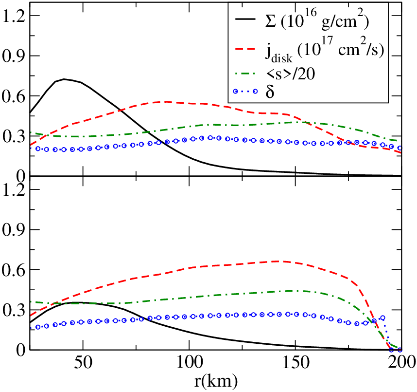
For inclined disks, we also measure the tilt and twist of the disk, as defined by Eq. (22). For large inclinations (s.5i60 and s.5i80), the tilt angle between the disk angular momentum and the orientation of the BH spin varies slowly during the evolution of the disk, at least in the higher density regions. Fig. 13 shows the tilt and twist profiles 20, 30 and 40ms after merger for simulation s.5i60. In the inner part of the disk (), the tilt decreases from to over those 20ms. The precession of the disk is more significant: we observe a variation of the twist of about over the same period. However, the precession rate is not constant at all radii and changes in time; the disk has not reached a state in which it precesses at a constant rate as one solid body. For smaller inclinations, relative variations in the tilt are larger. The inclination of the disk decreases at late-time to , and no global precession is observed.
An inclined disk showing some similarities with the results of our most inclined simulations (s.5i60 and s.5i80) was evolved in the presence of magnetic fields by Fragile et al. [40]. Even though the two simulations vary greatly in their initial conditions — Fragile et al. start their simulation from a torus of matter with peak density at () — the thickness and inclination of the disks are equivalent and some results from [40] could apply to the late time behavior of our disks. In Fragile et al., the inner disk is warped by the gravitomagnetic torque of the black hole, leading to larger tilts at lower radii. The same torque leads to a precession of the disk over a period of about 4s (for a black hole remnant of final mass ). This last effect is, however, acting over time scales longer than the lifetime of the disk formed in BHNS mergers, so that it seems unlikely that our disk would have time to reach the steady precession described in [40]. The magneto-rotational instability (MRI), on the other hand, appears to develop over roughly one orbital time scale, or about for the initial configuration chosen in [40] and a central black hole of mass . The rise of the MRI might be even faster for a disk more similar to the results of our simulations, as the peak of the density profile is significantly closer to the black hole in our disks than in [40], and the evolution time scale is thus shorter: the orbital period of circular orbits at is about 5ms. The MRI should have a strong influence on the redistribution of angular momentum in the fluid, and therefore on the accretion rate. However, the accretion rate is also influenced by the presence of shocks in the disk (see e.g. Fragile and Blaes [41] for shocks in tilted disks similar to [40]). This means that interactions between the disk and the matter falling back in the tidal tail are also likely to play an important role in the determination of the lifetime of the disk. Thus, both the magnetic effects and realistic initial conditions are required to accurately predict the lifetime of the disks resulting from BHNS mergers.

Lower panel: Twist profile for the same configuration. Over the 20ms of evolution, the disk goes through more than one fourth of a precession period.
VII Conclusions
Astrophysical BHNS binaries are expected to have BH spins that are not aligned with the orbital angular momentum of the system. We performed here the first fully general relativistic simulations of BHNS systems with precessing orbits. We find that for realistic inclinations of the BH spin with respect to the initial orbital angular momentum (), a mass ratio of 1:3, and a moderate black hole spin , the mass of the disk varies by about a factor of 2. More important, the inclination of the spin seems to have a significant impact on the final remnant only for . According to population synthesis models by Belczynski et al. [15], this means that, for binaries with initial spin of 0.5, half of the systems would have disks nearly as massive as if the BH spin was aligned with the orbital angular momentum of the system. This confirms the relevance of the aligned BHNS studies previously undertaken by ourselves and by other groups. At late times, the inclination of the disks formed in these precessing systems remain relatively modest (). Most of the angular momentum of the system is in the orbital motion of the binary, which precesses around the total angular momentum of the system at a small misalignment angle ( for ). The black hole spin axis itself is inclined at a larger angle to the total angular momentum, but its misalignment decreases as the hole accretes matter from the disrupted neutron star. This suggests that more inclined disks could be observed for larger black hole spins or more extreme mass ratios. Here, our most inclined binaries have an average tilt . From the results of Fragile et al. [40], we would expect those disks to precess as one solid body around the black hole — but only over time scales far longer than the expected lifetime of our post-merger disks ().
For spins aligned with the orbital angular momentum, our study shows qualitative agreement with previous results by Etienne et al. [12]. As expected, large spins favor the formation of a massive disk. By studying a higher initial spin (), we also show that large disks of mass can be obtained for .
All the cases studied here produce post-merger systems that are promising SGRB central engines. Despite large differences in the disk masses, the lifetime of the system seems mostly independent of the black hole spin; we find an accretion time scale for all cases. The disks have a peak surface density located about away from the hole, and extend about twice as far. They are always thick (), hot (MeV), and accreting at a super-Eddington rate (). All simulations also show the presence of a baryon-free region, at least at densities above the threshold at which atmospheric corrections begin to have an impact (). This region covers a cone with an opening angle of around the axis of the black hole spin, except for the high-spin configuration for which the disk is significantly closer to the BH, and the opening angle varies within the range . Such a region is required if relativistic jets are to be launched.
Accretion continues throughout the disk evolution, but the thermal and rotational profiles do seem to stabilize. The specific angular momentum of the disks increases with radius, so they are not subject to the Rayleigh instability. The angular velocity, however, decreases with radius, so these disks are subject to the magneto-rotational instability (MRI), an effect not included in our simulations.
The late-time behavior of the black hole-accretion disk system is critical if we want to understand the potential of BHNS mergers as progenitors for short gamma-ray bursts. Currently, the measurement of the properties of the disk and their evolution in time suffers from the limitations of our simulations. The general characteristics of the disk can be obtained, but a more detailed evolution would certainly require the inclusion of magnetic fields and neutrino radiation. These effects will be added to our evolutions in the near future.
Acknowledgements.
We thank Geoffrey Lovelace and Harald Pfeiffer for useful discussions and suggestions. This work was supported in part by a grant from the Sherman Fairchild Foundation, by NSF Grants Nos. PHY-0652952 and PHY-0652929, and NASA Grant No. NNX09AF96G. This research was supported in part by the NSF through TeraGrid [42] resources provided by NCSA’s Ranger cluster under Grant No. TG-PHY990007N. Computations were also performed on the GPC supercomputer at the SciNet HPC Consortium. SciNet is funded by: the Canada Foundation for Innovation under the auspices of Compute Canada; the Government of Ontario; Ontario Research Fund - Research Excellence; and the University of Toronto.References
- [1] ligo web page, http://www.ligo.caltech.edu.
- [2] ego-virgo web page, http://www.ego-gw.it.
- [3] ligo Scientific Colaboration and virgo Scientific Colaboration, Classical and Quantum Gravity 27, 173001 (2010), eprint 1003.2480v2.
- [4] B. Paczynski, Acta Astronomica 41, 257 (1991).
- [5] W. H. Lee and E. Ramirez-Ruiz, New Journal of Physics 9, 17 (2007), eprint arXiv:astro-ph/0701874.
- [6] M. Shibata and K. Uryu, Phys. Rev. D74, 121503 (2006), eprint gr-qc/0612142.
- [7] M. Shibata and K. Uryu, Class. Quant. Grav. 24, S125 (2007), eprint astro-ph/0611522.
- [8] M. Shibata and K. Taniguchi, Phys. Rev. D77, 084015 (2008), eprint 0711.1410.
- [9] M. Shibata, K. Kyutoku, T. Yamamoto, and K. Taniguchi, Phys. Rev. D79, 044030 (2009), eprint 0902.0416.
- [10] Z. B. Etienne, J. A. Faber, Y. T. Liu, S. L. Shapiro, K. Taniguchi, and T. W. Baumgarte, Phys. Rev. D 77, 084002 (2008), eprint 0712.2460.
- [11] M. D. Duez, F. Foucart, L. E. Kidder, H. P. Pfeiffer, M. A. Scheel, and S. A. Teukolsky, Phys. Rev. D 78, 104015 (2008), eprint 0809.0002.
- [12] Z. B. Etienne, Y. T. Liu, S. L. Shapiro, and T. W. Baumgarte, Phys. Rev. D79, 044024 (2009).
- [13] M. D. Duez, F. Foucart, L. E. Kidder, C. D. Ott, and S. A. Teukolsky, Classical and Quantum Gravity 27, 114106 (2010), eprint 0912.3528.
- [14] V. Ferrari, L. Gualtieri, and F. Pannarale, Phys. Rev. D 81, 064026 (2010), eprint 0912.3692.
- [15] K. Belczynski, R. E. Taam, E. Rantsiou, and M. van der Sluys, Astrophys. J. 682, 474 (2008), eprint arXiv:astro-ph/0703131.
- [16] E. Rantsiou, S. Kobayashi, P. Laguna, and F. A. Rasio, Astrophys. J. 680, 1326 (2008), eprint arXiv:astro-ph/0703599.
- [17] J. W. York, Phys. Rev. Lett. 82, 1350 (1999).
- [18] H. P. Pfeiffer, Ph.D. thesis, Cornell University (2003), arXiv:gr-qc/0510016v1.
- [19] H. P. Pfeiffer, L. E. Kidder, M. A. Scheel, and S. A. Teukolsky, Comput. Phys. Commun. 152, 253 (2003).
- [20] H. P. Pfeiffer, G. B. Cook, and S. A. Teukolsky, Phys. Rev. D 66, 024047 (2002).
- [21] F. Foucart, L. E. Kidder, H. P. Pfeiffer, and S. A. Teukolsky, Phys. Rev. D77, 124051 (2008).
- [22] G. Lovelace, R. Owen, H. P. Pfeiffer, and T. Chu, Phys. Rev. D78, 084017 (2008).
- [23] G. B. Cook and H. P. Pfeiffer, Phys. Rev. D 70, 104016 (2004).
- [24] H. P. Pfeiffer, D. A. Brown, L. E. Kidder, L. Lindblom, G. Lovelace, and M. A. Scheel, Classical and Quantum Gravity 24, S59 (2007), eprint arXiv:gr-qc/0702106.
- [25] http://www.black-holes.org/SpEC.html.
- [26] L. Lindblom, M. A. Scheel, L. E. Kidder, R. Owen, and O. Rinne, Class. Quant. Grav. 23, S447 (2006).
- [27] P. Colella and P. R. Woodward, Journal of Computational Physics 54, 174 (1984).
- [28] T. Yamamoto, M. Shibata, and K. Taniguchi, Phys. Rev. D78, 064054 (2008), eprint 0806.4007.
- [29] B. van Leer, J. Comput. Phys. 23, 276 (1977).
- [30] B. C. Stephens, S. L. Shapiro, and Y. T. Liu, Phys. Rev. D 77, 044001 (2008), eprint 0802.0200.
- [31] P. C. Fragile and P. Anninos, Astrophys. J. 623, 347 (2005), eprint arXiv:astro-ph/0403356.
- [32] M. Boyle, D. A. Brown, L. E. Kidder, A. H. Mroué, H. P. Pfeiffer, M. A. Scheel, G. B. Cook, and S. A. Teukolsky, Phys. Rev. D 76, 124038 (2007).
- [33] M. Campanelli, C. O. Lousto, Y. Zlochower, and D. Merritt, Physical Review Letters 98, 231102 (2007), eprint arXiv:gr-qc/0702133.
- [34] M. A. Scheel, H. P. Pfeiffer, L. Lindblom, L. E. Kidder, O. Rinne, and S. A. Teukolsky, Phys. Rev. D 74, 104006 (2006), eprint arXiv:gr-qc/0607056.
- [35] L. E. Kidder, Phys. Rev. D 52, 821 (1995), eprint arXiv:gr-qc/9506022.
- [36] M. Campanelli, C. O. Lousto, and Y. Zlochower, Phys. Rev. D 74, 041501 (2006), eprint arXiv:gr-qc/0604012.
- [37] G. Faye, L. Blanchet, and A. Buonanno, Phys. Rev. D 74, 104033 (2006), eprint arXiv:gr-qc/0605139.
- [38] http://www.black-holes.org/explore2.html.
- [39] K. G. Arun, A. Buonanno, G. Faye, and E. Ochsner, Phys. Rev. D 79, 104023 (2009), eprint 0810.5336.
- [40] P. C. Fragile, C. C. Lindner, P. Anninos, and J. D. Salmonson, Astrophys. J. 691, 482 (2009), eprint 0809.3819.
- [41] P. C. Fragile and O. M. Blaes, Astrophys. J. 687, 757 (2008), eprint 0807.2453.
- [42] C. Catlett et al., in Advances in Parallel Computing, edited by L. Grandinetti (IOS press, Amsterdam, 2007).