Virialization of high redshift dark matter haloes
Abstract
We present results of a study of the virial state of high redshift dark matter haloes in an N-body simulation. We find that the majority of collapsed, bound haloes are not virialized at any redshift slice in our study () and have excess kinetic energy. At these redshifts, merging is still rampant and the haloes cannot strictly be treated as isolated systems. To assess if this excess kinetic energy arises from the environment, we include the surface pressure term in the virial equation explicitly and relax the assumption that the density at the halo boundary is zero. Upon inclusion of the surface term, we find that the haloes are much closer to virialization, however, they still have some excess kinetic energy. We report trends of the virial ratio including the extra surface term with three key halo properties: spin, environment, and concentration. We find that haloes with closer neighbors depart more from virialization, and that haloes with larger spin parameters do as well. We conclude that except at the lowest masses (), dark matter haloes at high redshift are not fully virialized. This finding has interesting implications for galaxy formation at these high redshifts, as the excess kinetic energy will impact the subsequent collapse of baryons and the formation of the first disks and/or baryonic structures.
Keywords:
cosmology: dark matter galaxies: high-redshift1 Introduction
In the standard cold dark matter (LCDM) model, small Gaussian perturbations in the dark matter density field at early times provide the seeds for the formation of structure in the Universe. The dark matter gravitationally collapses, and forms bound structures that eventually relax into a state of virial equilibrium. The number density of collapsed dark matter haloes at a given mass and epoch, the mass function, of these relaxed haloes provides powerful constraints on the parameters of the LCDM model (Haiman et al., 2001; Cunha & Evrard, 2010, see e.g. ). Various analytical methods (Press & Schechter, 1974; Bond et al., 1991; Sheth & Tormen, 1999, e.g. ) also predict the halo mass function for collapsed, bound, and virialized haloes in LCDM. However, simulations at high redshift () have found that the majority of collapsed, bound haloes are not in virial equilibrium (Jang-Condell & Hernquist, 2001; Hetznecker & Burkert, 2006; Davis & Natarajan, 2010). Thus, there seems to be a mis-match with simulations; they find mass functions (which assume the haloes are virialized) that match the analytic predictions, and yet the detailed structure of the haloes shows that they are not virialized. In this paper, we explore in detail the virialization state of dark matter haloes at high redshift in order to understand this discrepancy.
For an isolated collapsed, bound dark matter halo in equilibrium, the scalar virial theorem,
| (1) |
provides a simple relationship between the halo’s total kinetic () and potential () energies. In LCDM, dark matter haloes are expected to reach virial equilibrium rapidly upon collapse when they detach from the Hubble flow. The timescale for virialization is of the order of the dynamical time, which for a dark matter halo may be estimated as , where is the virial radius and the circular velocity, . For a halo at this is roughly , or one percent of the Hubble time at that redshift. Therefore, despite rapid merging activity these haloes have had sufficient time to reach virial equilibrium, but do not appear to do so in the simulations.
Here we explore the energy budget of these haloes, to determine why simulated haloes at high redshift are apparently out of virial equilibrium. There are several possibilities which may explain this finding. In this paper, we probe this issue by relaxing two assumptions typically made when applying the virial theorem. First, we include the non-negligible contributions of the environment to the halo’s gravitational potential and secondly, we do not truncate the density profile of the halo at the virial radius. While these two assumptions are valid for isolated haloes typical of the local Universe, at high redshift when the Universe was denser, these assumptions are incorrect. In addition to these two assumptions, it is possible that systematic errors from the halo finding algorithm may bias measurements of halo virialization. Finally, we explore the possibility that the departure from virialization is correlated with key halo properties. The organization of this paper is as follows: we derive the virial equation from the momentum equation in section 2, explicitly retaining the surface terms that are usually neglected. In section 3 present simulation results and the correlations between halo energetics and key halo structural properties, namely, halo spin, concentration, and local environment. We conclude in section 4 with a discussion of our findings and their implications.
2 The Virial Equation
Here we derive the virial theorem for dark matter haloes including boundary effects and an external gravitational potential. An isolated system of collisionless particles in equilibrium satisfies the scalar virial theorem (see Equation 1). This result is derived under the assumption that the mass density approaches zero at large radii for a finite mass distribution. In this work, our systems of interest are high redshift dark matter haloes, which form within a cosmic web of sheets, voids, and filaments. We therefore cannot assume that the mass density approaches zero at the boundary of these systems. We also consider the potential due to nearby particles exterior to the haloes.11 1 In what follows, we use the Einstein summation convention where repeated indices correspond to summations.
The virial theorem is obtained from the conservation of momentum for a dark matter halo modeled as a collisionless fluid. Following Binney & Tremaine (1987), the corresponding fluid equation is multiplied by and integrated over the volume , with the caveat that the surface terms resulting from integration by parts do not vanish. In this case, the tensor virial theorem corresponding to a collisionless fluid is given by,
| (2) |
where is the moment of inertia tensor, is the kinetic energy tensor, is the potential energy tensor. We denote the mass density, position, average velocity, and gravitational potential by , , , and respectively. The vector is the outward-pointing unit normal to the surface that encloses the volume . The third term on the right of equation (2) corresponds to the kinetic stresses on the halo boundary. The last term is the time derivative of the moment of inertia flux through the surface (Ballesteros-Paredes, 2006). The scalar virial theorem is obtained by taking the trace of equation (2):
| (3) |
Following Binney & Tremaine (1987) and Ballesteros-Paredes (2006), the potential energy term may be broken up into contributions from particles inside and outside of the halo, , so that
| (4) |
Note that the first term is the gravitational potential energy of the halo, which we denote as from here on. In the case of a spherical volume, the last term in equation (3) is , where is the radius and is the mass enclosed within the volume. Assuming that this term is negligible for a steady-state system, we obtain
| (5) | |||||
| (6) | |||||
| (7) |
for a halo in virial equilibrium. and represent corrections to the standard virial relation and can be explicitly calculated for simulated dark matter haloes.
3 Simulation Results
Using GADGET-2 (Springel, 2005), we ran a dark matter only simulation with the WMAP5 cosmological parameters (Dunkley et al., 2009, {} = {0.258, 0.742, 0.044, 0.719, 0.963, 0.796},) from to (see Davis & Natarajan (2010) for full details). Our dark matter particle mass is , which sets a comoving box size at , with dark matter particles. We use the HOP algorithm to identify collapsed dark matter haloes (Eisenstein & Hut, 1998). HOP first calculates a density for each particle by smoothing over its nearest 64 neighbors using a cubic spline kernel. It then groups particles with their densest neighbor, and density thresholds are used to ensure that haloes are not being over-counted as sub-haloes within a larger halo. We choose density thresholds to match the high redshift mass function described in Reed et al. (2007). Lastly, we remove unbound particles from each halo.
For each halo, we calculate the total potential energy, , using a direct summation over the particles assigned to the halo:
| (8) |
where is the separation between particles and , is Newton’s gravitational constant, and the particle mass. The total kinetic energy, is found by summing over the particle’s individual kinetic energies:
| (9) |
In measuring and , we must ensure that we have enough particles in our halo sample to accurately measure the energies. We addressed this question in Davis & Natarajan (2010), and summarize the relevant points here. We re-ran our simulation with one eighth as many particles ( total) and with eight times as many particles ( total). This allows us to compare directly individual halos with different resolutions. We used the halo centre of mass to cross-matched the halo catalogues. We show in Figure 1 the change in and for the and runs as a function of the number of particles in the low resolution halo. We find that at least particles are required to accurately measure the kinetic and potential energies, and restrict our halo sample to halos with at least this many particles, corresponding to a halo mass of .


Having measured the kinetic and potential energies of our haloes, we can define the virial ratio,
| (10) |
which for fully virialized haloes should be zero. However, as our measurements of and are instantaneous quantities, and not time averaged, we expect a range of values for , with a mean value of zero. There are various cuts on used in the literature to select strictly virialized haloes: Shaw et al. (2006) use , Bett et al. (2007) use , and Neto et al. (2007) use . As noted in Davis & Natarajan (2010) we find that our haloes do not have , but are offset to high values of kinetic energy such that for all redshifts, and haloes are further from virialization at higher redshifts. One possibility is that the extra terms in the virial equation ( and ) are not negligible at higher redshifts, where large amounts of infalling material contribute to the terms. As the Universe expands, we expect a smaller contribution from these extra terms. Our findings follow the general trend reported in Hetznecker & Burkert (2006) at lower redshift, though their fitting function cannot be extended to our redshift range.
The virialization process is expected to happen from the inside out. Thus, it should be possible to identify a virialized core. To do this, we calculated and only for particles inside three smaller radii: and For the choice of boundary at , we do find virialized cores, as expected. We show in Figure 2 histograms of for these three inner radii as well as the histogram of for the entire halo. We find that for smaller radii, the mean value of shifts towards , as expected for a virialized object. Thus we conclude that the halo cores of our sample are virialized, while the entire halo is not.

The departure from virial equilibrium motivated our interest in the extra terms in the virial equation. We calculate the contribution to the potential energy from the external mass distribution, (equation 6). Converting the volume integral into a sum over particles, we find
| (11) |
where is the total number of particles in the halo (see equation 11). To calculate the gravitational acceleration acting on particle we sum over all particles, , within which are not part of the halo itself:
| (12) |
However, after calculating this term, we find that it is negligible compared to (of order ). Thus, even at higher redshifts where it may be expected that external matter will affect the total gravitational term in the virial equation, we find that it provides only a small contribution to the total energy.
We next examine the term in equation 7, . Following Shaw et al. (2006) , we select halo particles between and , where is the radius which encloses a mean overdensity of . This defines the surface over which we perform the summation. Then, approximating the surface integral as a summation over particles in this shell, we calculate as:
| (13) |
where is the mean radius of the particles in the shell of thickness . Each particle, , has a radial velocity . We note that our term is similar to that of Shaw et al. (2006), but not identical to their surface pressure term. Here we included only the contribution from the velocity component normal to the surface. This may be important if the velocities of the particles falling into the halo are on predominantly radial orbits, such as falling into the halo along a filament, and would then have a larger surface term than when simply calculating the total pressure (which is proportional to ). We find that at least particles are required in the shell to correctly resolve and calculate ; haloes with fewer particles have strongly biased (low) values of . We therefore only include haloes with more than 30 particles in this shell for the remainder of this work.
We point out that our halos are not spherical – there is no guarantee that the density cuts used by the HOP algorithm yields spherical halos. However, in our calculation of , we have chosen a spherical surface over which to measure this term. Thus, we wish to test whether there is any bias in the value of arising from the real shapes of haloes. To measure halo shapes, we use the same method as in Davis & Natarajan (2010). First, we calculate the normalized moment of inertia tensor. The ratios of the eigenvalues () of this tensor can be used to define a halo’s sphericity () and triaxiality (). We found, however, no trend between shape and or . Thus, we conclude that our choice of using a spherical shell rather than following the outer boundary of the HOP halo does not bias our results.

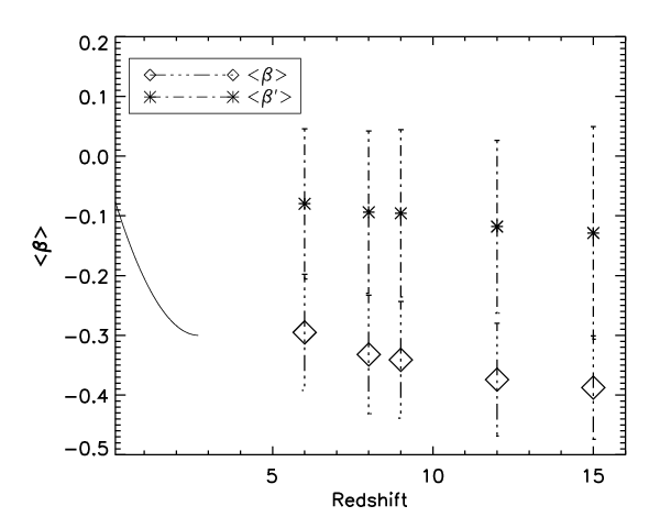
Having found that is negligible, we now include only the surface pressure term, , in our calculation of a corrected virial ratio, , where:
| (14) |
and show in the top panel of Figure 3, a histogram of and at . Without including the term, we find , and after inclusion, we find . The standard deviation of the corrected distribution increases slightly, from to . With the inclusion of , we find that the virial theorem is nearly satisfied by our haloes at : approximately lie within the cut applied by Shaw et al. (2006) of , whereas only of the haloes have .
At higher redshifts, however, becomes increasingly negative, implying that our haloes are farther from virialization at higher redshift even after the correction arising from the surface term is taken into account. This is to be expected, as these haloes have had less time to fully relax. We show in the bottom panel of Figure 3 and as a function of redshift. We include as the solid curve the fitting function of Hetznecker & Burkert (2006)22 2 Note that there is a typo in their fitting function as reported in their paper. It should read , where . which they found for redshifts less than . We find that the correction term, does not fully correct the virial ratio at any redshift, and the in fact correction is less effective at higher redshifts as seen in Figure 3.
3.1 Correlation of with halo properties
After including the extra term, from the virial equation, we have found that the haloes still do not have a mean of zero as expected. We compare to other halo properties, in an attempt to find the source of the offset.
The effect of the local environment is first examined, as it addresses the assumption of isolation in the virial theorem. In a recent paper Davis & Natarajan (2010) studied correlations between the local environment and halo structural properties. We use one of their metrics of the local environment, the distance to the nearest neighbor (D3), and compare it with the virial ratios, and . We expect that haloes in denser environments and with close neighbors will have larger surface terms, as these haloes are least likely to be in isolation as is assumed by the standard virial theorem. Thus we expect a trend with and environment, and after accounting for the surface terms, any remaining correlation could explain the increased dispersion seen in compared to .
We find that for extremely unvirialized haloes such that , the mean value of D3 is with a standard deviation of . We note here that our box size at this epoch is kpc. However, for the full sample of haloes, the mean distance is with . Thus, the extremely unvirialized haloes are slightly systematically closer to other haloes. In Figure 4 we show the correlation between and D3 at ; the solid curve shows the mean value of D3 binned by with error bars depicting the error of the mean, and the dashed curve shows a linear fit to the mean trend with a slope and y-intercept . The fit has a reduced . There is only a slight trend for haloes with small values of to have closer neighbors than halos with large values of . However, there is large scatter in the values of D3 in a given range of , implying that environment is not the only factor in the dispersion of .
Hetznecker & Burkert (2006) report a correlation between the spin parameter,
and their definition of the virial coefficient, . They found that for redshifts between , is proportional to , and that the relationship varied with redshift. As they note, we expect a relationship between and , with scatter due to the angular momentum, , in the definition of . When we use their definition of , we find similar results, but this definition does not account for the surface term of equation 13. We show in Figure 4 the correlation between and at . We report a similar trend to Hetznecker & Burkert (2006). For comparison, we fit our data to the same relationship: , and found best fit values of and , similar to the values Hetznecker & Burkert (2006) found of and for all haloes in their simulation between .
In Davis & Natarajan (2010) we fit NFW profiles to our halo sample at . Using the scale radius from the fit, we define the halo concentration, . In this work, we look for a correlation between halo concentration and . Analytic models of dark matter haloes with galaxy and cluster scale masses at low redshift and which use the NFW density profile find that haloes with smaller concentrations are further from virialization () Lokas & Mamon (2001). For these massive haloes, simulations run by Shapiro et al. (2004) match the analytic trends predicted by Lokas & Mamon (2001). We find, however, that our halo sample does not follow the same trend reported in Lokas & Mamon (2001). Our simulations show that haloes which are virialized () have smaller concentrations than haloes with .
Another method of finding relaxed haloes is to use the offset between the center of mass and the center of the potential well (D’Onghia & Navarro, 2007, see e.g.). We use the location of the densest particle in the halo as a proxy for the center of the halo’s potential well, and compare this offset, , to . We find a small trend for haloes with small values of to have larger offsets, as shown in Figure 4 for the haloes at . However, we note that there does not seem to be a systematic shift in for haloes with . Thus, we conclude that using to find virialized haloes is not effective at these redshifts.


4 Discussion
In this paper, we explore the question of whether or not high redshift dark matter haloes are virialized. Including the surface term in the virial equation, of our haloes at are virialized () whereas without the term, only of them are. However, the distribution of virial ratios is still not centered around . A mean of would be expected if the spread of is due simply to the fact that our measurements of the kinetic and potential energies are not time-averaged. Therefore, we conclude that simulated dark matter haloes at high redshifts are not virialized. On average, they have too much kinetic energy. One explanation for this excess kinetic energy is due to the approximations that we have made in calculating the terms in the virial theorem. A key issue is the choice of the shell in calculating , which is arbitrary. It needs to be large enough so that we can sufficiently resolve the flux through the shell. However, with better particle resolution, the shell could be narrowed for a better approximation to the surface integral. We have also fixed the shell as spherical, whereas the haloes are not truly spherical. Also, because of the time resolution of our snapshots, we are not able to test if the moment of inertia flux (the last term in equation 3) is truly negligible.
Our findings could be a consequence of the deployed halo finding algorithms at high redshifts. Since virialization happens from the inside out, it is possible to find a virialized core by looking at regions interior to the standard definition of the virial radius. This would be necessary if one seeks to find fully virialized sets of particles at high redshift. Altering the halo finder would however, alter the mass function derived from our simulations, which would put it out of line with mass functions from other simulations at similar redshifts (Reed et al., 2007) and from analytic predictions.
Finally, our finding has important implications for galaxy formation. Haloes with excess kinetic energy will mostly likely also have increased turbulence when baryonic gas falls into the central regions of the halo. The ensuing turbulent viscosity could be an effective method for transporting angular momentum in high redshift dark matter haloes. This might alter the cooling and collapse of baryons in these high redshift haloes than expected, as suggested in recent results reported by Grief et al. (2011).
Acknowledgements
We are grateful for the helpful comments of the referee. We also thank Laurie Shaw for many helpful discussions. This work was supported in part by the facilities and staff of the Yale University Faculty of Arts and Sciences Hight Performance Computing Center.
References
- Ballesteros-Paredes (2006) Ballesteros-Paredes J., 2006, MNRAS, 372, 443
- Bett et al. (2007) Bett P., Eke V., Frenk C. S., Jenkins A., Helly J., Navarro J., 2007, MNRAS, 376, 215
- Binney & Tremaine (1987) Binney J., Tremaine S., 1987, Galactic dynamics. Princeton, NJ, Princeton University Press, 1987, 747 p.
- Bond et al. (1991) Bond J. R., Cole S., Efstathiou G., Kaiser N., 1991, ApJ, 379, 440
- Cunha & Evrard (2010) Cunha C. E., Evrard A. E., 2010, Phys Rev D, 81, 083509
- Davis & Natarajan (2010) Davis A. J., Natarajan P., 2010, MNRAS, 407, 691
- D’Onghia & Navarro (2007) D’Onghia E., Navarro J. F., 2007, MNRAS, 380, L58
- Dunkley et al. (2009) Dunkley J., Komatsu E., Nolta M. R., Spergel D. N., Larson D., Hinshaw G., Page L., Bennett C. L., Gold B., Jarosik N., Weiland J. L., Halpern M., Hill R. S., Kogut A., Limon M., Meyer S. S., Tucker G. S., Wollack E., Wright E. L., 2009, ApJS, 180, 306
- Eisenstein & Hut (1998) Eisenstein D. J., Hut P., 1998, ApJ, 498, 137
- Grief, White, Klessen & Springel (2011) Grief, T., White, S., Klessen, R., Springel, V., 2011, ArXiv Astrophysics e-prints 1101.5493
- Haiman et al. (2001) Haiman Z., Mohr J. J., Holder G. P., 2001, ApJ, 553, 545
- Hetznecker & Burkert (2006) Hetznecker H., Burkert A., 2006, MNRAS, 370, 1905
- Jang-Condell & Hernquist (2001) Jang-Condell H., Hernquist L., 2001, ApJ, 548, 68
- Lokas & Mamon (2001) Lokas E. L., Mamon G. A., 2001, MNRAS, 321, 155
- Neto et al. (2007) Neto A. F., Gao L., Bett P., Cole S., Navarro J. F., Frenk C. S., White S. D. M., Springel V., Jenkins A., 2007, MNRAS, 381, 1450
- Press & Schechter (1974) Press W. H., Schechter P., 1974, ApJ, 187, 425
- Reed et al. (2007) Reed D. S., Bower R., Frenk C. S., Jenkins A., Theuns T., 2007, MNRAS, 374, 2
- Shapiro et al. (2004) Shapiro P. R., Iliev I. T., Martel H., Ahn K., Alvarez M. A., 2004, ArXiv Astrophysics e-prints 0409173
- Shaw et al. (2006) Shaw L. D., Weller J., Ostriker J. P., Bode P., 2006, ApJ, 646, 815
- Sheth & Tormen (1999) Sheth R. K., Tormen G., 1999, MNRAS, 308, 119
- Springel (2005) Springel V., 2005, MNRAS, 364, 1105