The Carter Constant for Inclined Orbits About a Massive Kerr Black Hole: I. circular orbits

P. G. Komorowski* S. R. Valluri*# M. Houde*

Abstract

In an extreme binary black hole system, an orbit will increase its angle of inclination ( ${\iota}$ ) as it evolves in Kerr spacetime. We focus our attention on the behaviour of the Carter constant ( ${Q}$ ) for near-polar orbits; and develop an analysis that is independent of and complements radiation reaction models. For a Schwarzschild black hole, the polar orbits represent the abutment between the prograde and retrograde orbits at which ${Q}$ is at its maximum value for given values of latus rectum ( ${\tilde{l}}$ ) and eccentricity ( ${e}$ ). The introduction of spin ( ${\tilde{S}}={\left|\mathbf{J}\right|}/{M}^{2}$ ) to the massive black hole causes this boundary, or abutment, to be moved towards greater orbital inclination; thus it no longer cleanly separates prograde and retrograde orbits.

To characterise the abutment of a Kerr black hole (KBH), we first investigated the last stable orbit (LSO) of a test-particle about a KBH, and then extended this work to general orbits. To develop a better understanding of the evolution of ${Q}$ we developed analytical formulae for ${Q}$ in terms of ${\tilde{l}}$ , ${e}$ , and ${\tilde{S}}$ to describe elliptical orbits at the abutment, polar orbits, and last stable orbits (LSO). By knowing the analytical form of $\partial{Q}/\partial{\tilde{l}}$ at the abutment, we were able to test a 2PN flux equation for Q. We also used these formulae to numerically calculate the $\partial{\iota}/\partial{\tilde{l}}$ of hypothetical circular orbits that evolve along the abutment. From these values we have determined that $\partial{\iota}/\partial{\tilde{l}}=-\left(122.7{\tilde{S}}-36{\tilde{S}}^{3}\right){\tilde{l}}^{-11/2}-\left(63/2\,{\tilde{S}}+35/4\,{\tilde{S}}^{3}\right){\tilde{l}}^{-9/2}-15/2\,{\tilde{S}}{\tilde{l}}^{-7/2}-9/2\,{\tilde{S}}{\tilde{l}}^{-5/2}$ . By taking the limit of this equation for ${\tilde{l}}\rightarrow\infty$ , and comparing it with the published result for the weak-field radiation-reaction, we found the upper limit on $\left|\partial{\iota}/\partial{\tilde{l}}\right|$ for the full range of ${\tilde{l}}$ up to the LSO. Although we know the value of $\partial{Q}/\partial{\tilde{l}}$ at the abutment, we find that the second and higher derivatives of ${Q}$ with respect to ${\tilde{l}}$ exert an influence on $\partial{\iota}/\partial{\tilde{l}}$ . Thus the abutment becomes an important analytical and numerical laboratory for studying the evolution of ${Q}$ and ${\iota}$ in Kerr spacetime and for testing current and future radiation back-reaction models for near-polar retrograde orbits.

*Department of Physics and Astronomy, #Department of Applied Mathematics, University of Western Ontario, London, Ontario

1 Introduction

In his landmark work of 1968, Brandon Carter derived a new constant of motion that pertained to orbital motion in the gravitational field of a Kerr black hole (KBH) [1]. In due course, this constant became known as the Carter constant, which joins the set of important constants of motion: orbital angular momentum ( ${L}_{z}$ , ${z}$ -axis projection), orbital energy ( ${E}$ ), and finally the Carter constant ( ${Q}$ ). These constants of motion can be developed rigorously from the Hamilton-Jacobi equation [1, 2, 3].

An extreme mass ratio binary black hole system is composed of a secondary object (which may be a compact object (CO) of several solar masses) in orbit around a primary object (which is a massive black hole (MBH) of several million solar masses). Extreme mass ratio inspirals (EMRIs) are expected to emit gravitational wave radiation (GW) of sufficiently high energy and in the appropriate frequency band for detection by the Laser Interferometer Space Antenna (LISA) to be feasible [4, 5, 6, 7]. The emission of GW causes the constants of motion to evolve, which in turn affects the GW power spectrum. Therefore some useful methods have been developed to describe this evolution. For example, the quadrupole formalism [8, 9, 10, 11] and the Teukolsky equation [12, 13, 14] have yielded important results. The analytical description of the evolution of ${Q}$ has been more difficult to achieve than it has for the other two constants of motion [15]; although the use of the Teukolsky equation has shown great promise [16, 15, 4, 5, 7] in this endeavour.

As the CO inspirals, the gravitational radiation reaction causes the value of ${Q}$ to change [16, 17, 18, 15, 4, 19, 20, 21, 5, 22, 7]. Therefore a non-equatorial orbit lists as its angle of inclination, ${\iota}$ , increases with respect to time; a near-polar prograde orbit becomes polar, and ultimately retrograde [23, 17]. Such listing behaviour of an inclined orbit has been studied and confirmed using the most current Teukolsky-based fluxes [22]. It is our goal to develop an analytical and numerical methodology for testing and improving radiation reaction models for predicting orbit listing and inspirals for near-polar orbits.

Our interest lies in studying KBH systems; yet, the Schwarzschild black hole (SBH) is an important datum. An infinitesimal amount of spin angular momentum ( ${\delta}{\tilde{S}}\ll 1$ ) may be imparted to an MBH such that, for practical purposes, it can be regarded as an SBH (by virtue of its minuscule effect on the surrounding spacetime); and yet, the spherical symmetry of the system has been broken and a ${z}$ -axis defined. Then an SBH can be considered to have a prograde or retrograde inclined orbit; and the set of polar orbits define the abutment, at which ${Q}$ will be at its maximum value ( ${Q}$ is non-negative for any bound orbit), for given values of ${\tilde{l}}$ , ${e}$ , and ${\tilde{S}}$ (ceteris paribus).

In section 2 the motion of a test-particle in an inclined orbit is analysed from first principles [24, 25, 26, 27] to yield the effective radial potential and an analytical expression of ${\tilde{L}}_{z}$ for a last stable orbit (LSO). In section 3 we continue our analysis to find the roots of the effective radial and polar-angle potentials and use them to derive analytical expressions for ${\tilde{E}}$ and ${X}^{2}$ (where ${X}={\tilde{L}}_{z}-{\tilde{S}}{\tilde{E}}$ ). The concept of the abutment is then refined. In section 4, we derive a set of critical formulae that express ${Q}$ at the LSO, along the abutment, and for the set of polar orbits. The interrelationships between these formulae are examined and a map of admissible values of ${Q}$ , with respect to ${\tilde{l}}$ and ${e}$ is drawn. In section 5, this map is used to better understand the path in the ${Q}$ - ${\tilde{l}}$ plane that is followed by an evolving circular orbit. We demonstrate the importance of the first and second derivatives of ${Q}$ (on the abutment) with respect to ${\tilde{l}}$ for understanding the rate of change of ${\iota}$ as the orbit lists.

We shall use geometrical units by setting the speed of light and gravitational constant to unity (i.e. ${c}=1$ and ${G}=1$ ); therefore, mass-energy is in units of time (seconds). In addition, many of the parameters we use will be normalised with respect to the mass of the black hole ( ${M}$ ) or with respect to the test-particle mass ( ${m}$ ). In appendix A, the symbols used in this paper are tabulated. By emphasising normalised variables, the analytical equations and numerical formalism are much better handled.

2 The Motion of a Test-Particle in an Inclined Orbit

A sound mathematical analysis can be made on the assumption that the secondary body is of infinitesimal mass (i.e. a test-particle). In such a case, the background metric of the MBH dominates. In the case of EMRIs, the small ratio of the CO mass to the MBH mass ( ${\eta}\lessapprox 10^{-5}$ ) warrants our use of idealised test-particle calculations [4, 28, 5, 7].

2.1 Basic orbital equations

We begin by considering a test-particle in orbit about a KBH of arbitrary spin, ${\tilde{S}}$ , for which the four-momentum can be given the general definition [29],

\displaystyle P_{\gamma}

\displaystyle=

\displaystyle\biggl[-{m}{\tilde{E}},\>m\frac{{\tilde{\Sigma}}}{{\tilde{\Delta}}}\left({\it\frac{dR}{d\tilde{\tau}}}\right),\>{m}{M}{\tilde{L}}_{\theta},\>{m}{M}{\tilde{L}}_{z}\biggr],

(1)

where

\displaystyle{\tilde{\Delta}}

\displaystyle=

\displaystyle\left({R}^{2}-2\,R+{\tilde{S}}^{2}\right)

(2)

and

\displaystyle{\tilde{\Sigma}}

\displaystyle=

\displaystyle{\left(R^{2}+\tilde{S}^{2}{\cos^{2}\left(\theta\right)}\right)}.

(3)

Unlike the analysis in Komorowski et al. [29], we shall use normalised variables at the outset and offer a more thorough treatment. Because we are now considering inclined elliptical orbits, one cannot simplify the four-momentum by setting ${\tilde{L}}_{\theta}=0$ . But by knowing the Carter constant in terms of normalised variables (i.e. obtained by dividing through by ${m}{M}$ ),

\displaystyle{Q}

\displaystyle=

\displaystyle{\frac{\cos^{2}\left(\theta\right){\tilde{L}_{{z}}}^{2}}{\sin^{2}\left(\theta\right)}}+{\tilde{L}_{{\theta}}}^{2}+\cos^{2}\left(\theta\right){\tilde{S}}^{2}\left(1-{\tilde{E}}^{2}\right),

(4)

one can obtain the component of orbital angular momentum, ${\mathbf{L}}$ , projected upon the equatorial plane of the KBH,

\displaystyle{\tilde{L}}_{\theta}

\displaystyle=

\displaystyle\sqrt{{Q}-{\frac{\cos^{2}\left(\theta\right){\tilde{L}_{{z}}}^{2}}{\sin^{2}\left(\theta\right)}}-\cos^{2}\left(\theta\right){\tilde{S}}^{2}\left(1-{\tilde{E}}^{2}\right)},

(5)

and substitute it into the expression for the four-momentum:

	$\displaystyle P_{\gamma}$	$\displaystyle=$			(6)
		$\displaystyle\biggl[-{m}{\tilde{E}},m\frac{{\tilde{\Sigma}}}{{\tilde{\Delta}}}\left({\it\frac{dR}{d\tilde{\tau}}}\right),{m}{M}{\sqrt{{Q}-{\frac{\cos^{2}\left(\theta\right){\tilde{L}_{{z}}}^{2}}{\sin^{2}\left(\theta\right)}}-\cos^{2}\left(\theta\right){\tilde{S}}^{2}\left(1-{\tilde{E}}^{2}\right)}},{m}{M}{\tilde{L}}_{z}\biggr].$			(6)

The invariant quantity,

\displaystyle\vec{P}\cdot\vec{P}

\displaystyle=

\displaystyle\left.P_{\gamma}P_{\delta}g^{\delta\gamma}\right|_{Kerr}=-{m}^{2},

(7)

is calculated tensorially using the inverse Kerr metric (see Appendix B) and used to develop the radial orbital equation for a test-particle:

$\displaystyle{\tilde{\Sigma}}^{2}{\left(\frac{dR}{d\tilde{\tau}}\right)}^{2}$	$\displaystyle=$	$\displaystyle-\left({1-{\tilde{E}}^{2}}\right){R}^{4}+2\,{R}^{3}$	(8)
	$\displaystyle-$	$\displaystyle\left({\tilde{L}_{z}}^{2}+{\tilde{S}}^{2}{\left(1-{\tilde{E}}^{2}\ \right)}+Q\right){R}^{2}$
	$\displaystyle+$	$\displaystyle 2\,\left(\left({\tilde{L}_{z}-{\tilde{S}}{\tilde{E}}}\right)^{2}+Q\right)R-{Q{\tilde{S}}^{2}}.$

By setting ${Q}=0$ , equation (8) reduces to the equation for an equatorial orbit (see [20])

At the radial turning points, $d{R}/d{\tilde{\tau}}=0$ . Equation (8) becomes:

$\displaystyle 0$	$\displaystyle=$	$\displaystyle{R}^{4}-2\,{\frac{{R}^{3}}{1-{\tilde{E}}^{2}}}$	(9)
	$\displaystyle+$	$\displaystyle{\frac{\left({\tilde{L}_{z}}^{2}+{\tilde{S}}^{2}{\left(1-{\tilde{E}}^{2}\ \right)}+Q\right){R}^{2}}{1-{\tilde{E}}^{2}}}$
	$\displaystyle-$	$\displaystyle 2\,{\frac{\left(\left({\tilde{L}_{z}-{\tilde{S}}{\tilde{E}}}\right)^{2}+Q\right)R}{1-{\tilde{E}}^{2}}}+{\frac{Q{\tilde{S}}^{2}}{1-{\tilde{E}}^{2}}}.$

In the limit ${\tilde{S}}\rightarrow 0$ (set ${\tilde{S}}=0$ while retaining a non-zero value for ${Q}$ ) equation (9) becomes

\displaystyle 0

\displaystyle=

\displaystyle{R}^{4}-2\,{\frac{{R}^{3}}{1-{\tilde{E}}^{2}}}+{\frac{\left({\tilde{L}_{z}}^{2}+Q\right){R}^{2}}{1-{\tilde{E}}^{2}}}-2\,{\frac{\left({\tilde{L}_{z}}^{2}+Q\right)R}{1-{\tilde{E}}^{2}}}.

(10)

Thus, the square of the total orbital angular momentum, ${{\tilde{L}}^{2}}={\tilde{L}_{z}}^{2}+Q$ , confirms that, for the specific case of an SBH, ${Q}$ represents the square of the component of angular momentum projected on $x-y$ plane of the coordinate system (see Appendix B in Schmidt [30] and Appendix C in this paper for a more detailed treatment).

Some important research [21, 31] has been performed by working with the orbital inclination angle, ${\iota}$ , instead of ${Q}$ ; but in our study, the value of ${Q}$ will be taken as a system parameter. If ${Q}$ is chosen to be zero, then the orbital plane coincides with the equatorial plane of the KBH (i.e. ${\iota}=0$ and ${\theta}\equiv\pi/2$ ) and for a test-particle in a polar orbit (i.e. ${\iota}=\frac{\pi}{2}$ and $0\leq\theta\leq\pi$ ) ${\tilde{L}}_{z}$ must vanish. The choice of working directly with the Carter constant, ${Q}$ , as a system parameter is consistent with the approach taken by Carter [1] and more recently emphasised by others [32, 5, 22].

2.2 Effective Radial Potential

To proceed, we use a version of equation (8), which is quadratic in, ${\tilde{E}}$ ,

	$\displaystyle-R\left({R}^{3}+R{\tilde{S}}^{2}+2\,{\tilde{S}}^{2}\right){\tilde{E}}^{2}+4\,R\tilde{L}_{{z}}{\tilde{S}}{\tilde{E}}$
	$\displaystyle+R\left(R-2\right)\left(Q+{\tilde{L}_{{z}}}^{2}\right)+{R}^{2}\left({R}^{2}-2\,R+{\tilde{S}}^{2}\right)+Q{\tilde{S}}^{2}$	$\displaystyle=$	$\displaystyle 0.$		(11)

The roots of this equation can be used to determine the effective potential of the test-particle ( ${\tilde{V}}_{\pm}$ ):

	$\displaystyle{\tilde{V}}_{\pm}$	$\displaystyle=$	$\displaystyle\left(2\,R{\tilde{L}}_{{z}}\tilde{S}\pm\sqrt{{R}{Z}{\tilde{\Delta}}}\right)$		(12)
		$\displaystyle\times$	$\displaystyle\left(R\left({R}^{3}+{\tilde{S}}^{2}R+2\,{\tilde{S}}^{2}\right)\right)^{-1}$		(12)

where

\displaystyle{Z}

\displaystyle=

\displaystyle{R}^{5}+\left(Q+{\tilde{S}}^{2}+{\tilde{L}_{{z}}^{2}}\right){R}^{3}+2\,{R}^{2}{\tilde{S}}^{2}+{\tilde{S}}^{2}RQ+2\,Q{\tilde{S}}^{2}.

When the last stable orbit (LSO) is reached, ${\tilde{E}}$ corresponds to a local maximum of ${\tilde{V}}_{+}$ closest to the event horizon. Therefore one calculates the derivative of ${\tilde{V}}_{+}$ with respect to ${R}$ and equates it to zero, i.e.

$\displaystyle\frac{d{\tilde{V}}_{+}}{d{R}}$	$\displaystyle=-$	$\displaystyle\Biggl(2R\tilde{S}\tilde{L}_{{z}}\left(3\,{R}^{2}+{\tilde{S}}^{2}\right)\sqrt{{R}{Z}{\tilde{\Delta}}}+{R}^{3}{Z}_{1}{\tilde{L_{z}}^{2}}$	(13)
		$\displaystyle+\left({R}^{3}+{\tilde{S}}^{2}R+2\,{\tilde{S}}^{2}\right){Z}_{2}\Biggr)$
	$\displaystyle\times$	$\displaystyle\Biggl({R}\sqrt{{R}{Z}{\tilde{\Delta}}}{\left({R}^{3}+{\tilde{S}}^{2}R+2\,{\tilde{S}}^{2}\right)^{2}}\Biggr)^{-1}$
	$\displaystyle=$	$\displaystyle 0$

where

\displaystyle{Z}_{1}

\displaystyle={R}^{5}-3\,{R}^{4}+{\tilde{S}}^{2}{R}^{3}

\displaystyle-3\,{R}^{2}{\tilde{S}}^{2}+6\,{\tilde{S}}^{2}R-2\,{\tilde{S}}^{4},

and

	$\displaystyle{Z}_{2}$	$\displaystyle=$	$\displaystyle-{R}^{6}+{R}^{5}Q-\left(2\,{\tilde{S}}^{2}+3\,Q\right){R}^{4}+\left(2\,Q{\tilde{S}}^{2}+4\,{\tilde{S}}^{2}\right){R}^{3}$
		$\displaystyle-$	$\displaystyle\left({\tilde{S}}^{4}+2\,Q{\tilde{S}}^{2}\right){R}^{2}+{\tilde{S}}^{4}QR+{\tilde{S}}^{4}Q.$

2.3 Orbital Angular Momentum at the Last Stable Orbit

We can now develop an equation for the ${\tilde{L}}_{z}$ of a test-particle in an inclined orbit about a KBH (in a manner similar to that described in [29]) and extend the concept to general orbits. It should be noted, the value of ${\tilde{L}}_{z}$ considered here is not valid for general orbits, but pertains to the LSO. After eliminating the square root in equation (13) to yield a new equation that is quadratic in, ${{\tilde{L}}_{z}}^{2}$ , the solution is found to be:

	$\displaystyle{{\tilde{L}}_{z}}^{2}=\Bigl\{-{R}^{8}+\left(3+Q\right){R}^{7}+\left(-2\,{\tilde{S}}^{2}-6\,Q\right){R}^{6}$
	$\displaystyle+\left(\left(-6+2\,Q\right){\tilde{S}}^{2}+9\,Q\right){R}^{5}+\left(-{\tilde{S}}^{4}+\left(-10\,Q+12\right){\tilde{S}}^{2}\right){R}^{4}$
	$\displaystyle+\left(\left(-5+Q\right){\tilde{S}}^{4}+6\,Q{\tilde{S}}^{2}\right){R}^{3}-6\,{\tilde{S}}^{4}{R}^{2}Q$
	$\displaystyle+5\,{\tilde{S}}^{4}{R}Q-2\,{\tilde{S}}^{6}Q$
	$\displaystyle\pm 2{\tilde{S}}{\left(3\,{R}^{2}+{\tilde{S}}^{2}\right)}{\tilde{\Delta}}\sqrt{\left({R}^{5}-{R}^{4}Q+3\,{R}^{3}Q+{Q}^{2}{\tilde{S}}^{2}\right)}\Bigr\}$
	$\displaystyle\biggl({R}^{4}\left({R}^{3}+9\,R-4\,{\tilde{S}}^{2}-6\,{R}^{2}\right)\biggr)^{-1},$		(14)

which provides a relationship between ${\tilde{L}}_{z}$ and ${R}$ (which here, represents the pericentre radius) of the test-particle LSO. This result is independent of whether one begins the calculation with ${\tilde{V}}_{+}$ or ${\tilde{V}}_{-}$ .

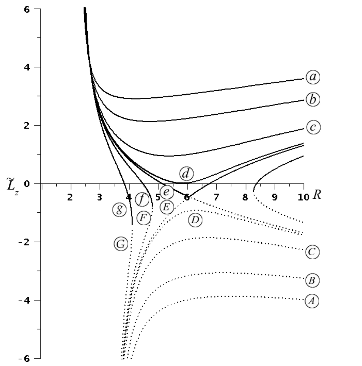
One can now plot ${\tilde{L}}_{z}$ with respect to the value of the pericentre (the point of closest approach, ${R}_{p}$ ) for an LSO for the cases where ${\tilde{S}}=0.0$ (Figure 1), ${\tilde{S}}=0.5$ (Figure 2) and ${\tilde{S}}=0.99$ (Figure 3). The values of ${\tilde{L}}_{z}$ calculated for an SBH are plotted in Figure 1 for the range of ${Q}$ values $0.0$ to ${16.0}$ .

For an SBH, the prograde (plus) and retrograde (minus) formulae for ${\tilde{L}}_{z}^{2}$ (equation (14)) are reflections of one another about the ${R}$ axis (Figure 1). But when ${\tilde{S}}>0$ , the plus equations are pulled below the ${R}$ axis and this symmetry is lost (Figures 2 and 3). There now exists a set of retrograde LSOs which are governed by the plus form of equation (14). The importance of this fact is revealed when we set the quantity beneath the square root in equation (14) to zero; i.e.

\displaystyle{R}^{5}-{Q}{R}^{4}+3{Q}{R}^{3}+{Q}^{2}{S}^{2}

\displaystyle=

\displaystyle 0.

(15)

The polynomial describes the boundary at which the plus and minus equations for ${\tilde{L}}_{z}^{2}$ are equal and it offers an insight into the behaviour of ${Q}$ for LSOs that are nearly polar ( ${\iota}\simeq\pi/2$ ). If ${\tilde{S}}=0$ , then for an elliptical LSO [33, 11, 29],

{R}_{p}=2\left(3+{e}\right)/\left(1+{e}\right).

(16)

By substituting equation (16) into equation (15) and solving for ${Q}$ , one obtains:

\displaystyle{Q}

\displaystyle=

\displaystyle 4\left(3+{e}\right)^{2}\left[\left(1+{e}\right)\left(3-{e}\right)\right]^{-1}.

(17)

This result applies to LSOs at the boundary and specifies an upper limit on ${Q}$ for orbits around an SBH. Now we must develop these ideas for general orbits about a KBH that have not yet reached their LSO.

3 Analysis of the Trajectory Equations

3.1 Introduction

There exist four trajectory equations [1, 34, 30] in two categories:

category (a)

(those that are periodic in radius, ${R}$ , or polar angle, ${\theta}$ )

{\tilde{\Sigma}}\frac{{dR}}{{d\tilde{\tau}}}=\pm\sqrt{{\tilde{V}}_{R}\left(R\right)}

(18)

{\tilde{\Sigma}}\frac{{d\theta}}{{d\tilde{\tau}}}=\pm\sqrt{{\tilde{V}}_{\theta}\left(\theta\right)}

(19)

category (b)

(those that are monotonically increasing in azimuthal angle, ${\varphi}$ , or coordinate time, ${t}$ )

{\tilde{\Sigma}}\frac{{d\phi}}{{d\tilde{\tau}}}={\tilde{V}}_{\phi}

(20)

{\tilde{\Sigma}}\frac{{d\tilde{t}}}{{d\tilde{\tau}}}={\tilde{V}}_{t}.

(21)

See Appendix B to see equations for functions ${\tilde{V}}_{R}\left({R}\right)$ , ${\tilde{V}}_{\theta}$ , ${\tilde{V}}_{\phi}$ , and ${\tilde{V}}_{t}$ . We have already developed equation (18) in section 2.1 (equation (8)). And equation (19) can also be developed by a similar method (see Appendix C).

One obtains, viz. equations (18) and (19), the following condition

\frac{{dR}}{{\sqrt{\tilde{V}_{R}\left(R\right)}}}=\frac{{d\theta}}{{\sqrt{\tilde{V}_{\theta}\left(\theta\right)}}},

(22)

on the geodesic of the test-particle, which is a general form of the equation specified by Schmidt (equation (16) in [30]). Given equation (19) [34], one can find the proper time of the orbit:

	$\displaystyle\tilde{\tau}$	$\displaystyle=$	$\displaystyle{\int_{{\theta}_{1}}^{{\theta}_{2}}}{\frac{{\tilde{\Sigma}d\theta}}{{\sqrt{{\tilde{V}}_{\theta}}}}}$		(23)
		$\displaystyle=$	$\displaystyle{\int_{{r}_{1}}^{{r}_{2}}}{\frac{{R^{2}dR}}{{\sqrt{{\tilde{V}}_{R}}}}}+{\tilde{S}^{2}}{\int_{{\theta}_{1}}^{{\theta}_{2}}}\frac{{\cos^{2}\left(\theta\right)}}{{\sqrt{{\tilde{V}}_{\theta}}}}d\theta,$		(23)

where the integral has been split into its separate ${R}$ and $\theta$ integral terms viz. equation (22). The same result is found when starting with equation (18) instead. Two other important integrals that can be calculated for coordinate time and azimuthal angle are given in Schmidt (equations (14) and (15) [30]) in which a detailed analysis is made on the basis of the Hamiltonian. Equation (23) can be solved to yield elliptic functions [20]; therefore, the roots of ${\tilde{V}}_{R}$ and ${V}_{\theta}$ contain information necessary for deriving analytical formulae for ${Q}$ in terms of ${\tilde{l}}$ and ${e}$ (for given ${\tilde{S}}$ ) and ${\iota}$ as a function of ${Q}$ . This will be shown in sections 3.3 and 4.

3.2 Roots of the Radial Equation

We introduce ${X}={\tilde{L}}_{z}-{\tilde{S}}{\tilde{E}}$ and convert equation (9) to the form:

$\displaystyle 0$	$\displaystyle=$	$\displaystyle{R}^{4}-2\,\frac{{R}^{3}}{\left({1-{\tilde{E}}^{2}}\right)}$	(24)
	$\displaystyle+$	$\displaystyle\frac{\left({X}^{2}+{\tilde{S}}^{2}+2{\tilde{S}}{\tilde{E}}{X}+Q\right){R}^{2}}{\left({1-{\tilde{E}}^{2}}\right)}$
	$\displaystyle-$	$\displaystyle\frac{2\,\left({X}^{2}+Q\right){R}}{\left({1-{\tilde{E}}^{2}}\right)}+\frac{{Q{\tilde{S}}^{2}}}{\left({1-{\tilde{E}}^{2}}\right)}.$

This substitution is consistent with the approach in [29] and that undertaken by Glampedakis and Kennefick [20]; and it will help us to derive the latus rectum of the LSO. Analytically, the use of ${X}^{2}$ in this case offers an advantage over the use of ${L}_{z}^{2}$ .

3.2.1 Elliptical Orbits.

By finding the four roots of equation (24) one can derive analytical formulae for ${X}$ and ${\tilde{E}}$ , in terms of ${e}$ , ${\tilde{l}}$ , ${Q}$ , and ${\tilde{S}}$ , which apply to general orbits (and are not limited to the LSO). Although the roots are easily obtained in terms of the constants of motion: ${\tilde{L}}_{z}$ , ${\tilde{E}}$ , and ${Q}$ ; they are complicated and as such not helpful. To simplify the analysis, we assume a priori that an inclined orbit can be characterised by an eccentricity, ${e}$ [35]. Therefore the radius of the orbit at its pericentre is described by

\displaystyle{r}_{p}

\displaystyle=

\displaystyle{\frac{{\tilde{l}}}{1+{e}}},

(25)

and correspondingly, at its apocentre

\displaystyle{r}_{a}

\displaystyle=

\displaystyle{\frac{{\tilde{l}}}{1-{e}}}.

(26)

To proceed, consider an expansion of the four possible roots $\left\{{r}_{4}<{r}_{3}\leq{r}_{p}\leq{r}_{a}\right\}$ :

$\displaystyle{R}^{4}$
$\displaystyle-\left(r_{{3}}+r_{{4}}+r_{{a}}+r_{{p}}\right){R}^{3}$
$\displaystyle+\left(r_{{4}}r_{{3}}+r_{{3}}r_{{a}}+r_{{3}}r_{{p}}+r_{{4}}r_{{a}}+r_{{4}}r_{{p}}+r_{{p}}r_{{a}}\right){R}^{2}$
$\displaystyle-\left(r_{{4}}r_{{3}}r_{{a}}+r_{{4}}r_{{3}}r_{{p}}+r_{{3}}r_{{p}}r_{{a}}+r_{{4}}r_{{p}}r_{{a}}\right)R$
$\displaystyle+r_{{4}}r_{{3}}r_{{p}}r_{{a}}$	$\displaystyle=$	$\displaystyle 0$	(27)

By equating the coefficients of the two polynomials in equations (24) and (27) one obtains the two independent equations:

\displaystyle{\frac{{\tilde{l}}\left(2\,r_{{4}}r_{{3}}+r_{{3}}{\tilde{l}}+r_{{4}}{\tilde{l}}\right)}{\left(1-{e}^{2}\right)}}

\displaystyle=

\displaystyle 2\,{\frac{{X}^{2}+Q}{1-{\tilde{E}}^{2}}},

(28)

and

\displaystyle{\frac{r_{{4}}r_{{3}}{\tilde{l}}^{2}}{1-{e}^{2}}}

\displaystyle=

\displaystyle{\frac{Q{\tilde{S}}^{2}}{1-{\tilde{E}}^{2}}},

(29)

which have been simplified viz. equations (25) and (26). Let us solve equations (28) and (29) to obtain:

\displaystyle{r}_{3}

\displaystyle=

\displaystyle{\frac{\left(1-{e}^{2}\right)}{{\tilde{l}}^{3}\left(1-{\tilde{E}}^{2}\right)}}\left[\left(Q\left(\tilde{l}-{\tilde{S}}^{2}\right)+{X}^{2}\tilde{l}\right)\pm\sqrt{{Z}_{3}}\right]

(30)

and

\displaystyle{r}_{4}

\displaystyle=

\displaystyle{\frac{Q{\tilde{S}}^{2}\left(1-{e}^{2}\right)}{{r}_{3}{\tilde{l}}^{2}\left(1-{\tilde{E}}^{2}\right)}}

(31)

where

	$\displaystyle{Z}_{3}$	$\displaystyle=$	$\displaystyle\left({\tilde{l}}-{\tilde{S}}^{2}\right)^{2}{Q}^{2}$
		$\displaystyle-$	$\displaystyle\tilde{l}\left({\frac{\left(1-{\tilde{E}}^{2}\right){\tilde{S}}^{2}{\tilde{l}}^{3}}{1-{e}^{2}}}-2\,{X}^{2}\tilde{l}+2\,{X}^{2}{\tilde{S}}^{2}\right)Q+{X}^{4}{\tilde{l}}^{2}.$

If ${Q}=0$ then selecting the minus sign in equation (30) yields ${r}_{3}=0$ ; therefore, the plus sign is the one taken as physically meaningful. For ${Q}=0$ , equation (30) reduces to

{r}_{3}=2\,{\frac{{X}^{2}\left(1-{e}^{2}\right)}{{\tilde{l}}^{2}\left(1-{\tilde{E}}^{2}\right)}},

(32)

which applies to an equatorial orbit. The value of ${r}_{4}$ equals zero when ${Q}=0$ as can be seen in equation (31).

3.2.2 Parabolic Orbits.

Parabolic orbits have importance to the empirical study of the interaction of stars with massive black holes (MBHs) [36, 37]. For parabolic orbits both ${e}=1$ and ${\tilde{E}}=1$ . We refer back to equation (24); and set ${\tilde{E}}=1$ :

$\displaystyle 0$	$\displaystyle=$	$\displaystyle{R}^{3}$	(33)
	$\displaystyle-$	$\displaystyle\frac{1}{2}\left({X}^{2}+{\tilde{S}}^{2}+2\,\tilde{S}X+Q\right){R}^{2}$
	$\displaystyle+$	$\displaystyle\left({X}^{2}+Q\right)R-\frac{1}{2}{Q{\tilde{S}}^{2}}.$

There are now three possible finite roots $\left\{{r}_{4}<{r}_{3}\leq{r}_{p}\right\}$ , which can be used in a new general equation ( ${r}_{a}$ is infinite in the case of a parabolic orbit):

	$\displaystyle{R}^{3}-\left(r_{{3}}+r_{{4}}+r_{{p}}\right){R}^{2}$
	$\displaystyle+\left(r_{{4}}r_{{3}}+r_{{3}}r_{{p}}+r_{{4}}r_{{p}}\right)R-r_{{4}}r_{{3}}r_{{p}}$	$\displaystyle=$	$\displaystyle 0.$		(34)

The pericentre simplifies (viz. ${{e}=1}$ ) to become,

\displaystyle{r}_{p}

\displaystyle=

\displaystyle{\frac{{\tilde{l}}}{2}};

(35)

and correspondingly, at its apocentre,

\displaystyle{r}_{a}

\displaystyle\rightarrow

\displaystyle\infty.

(36)

We obtain the solutions for the additional roots:

\displaystyle{r}_{3}

\displaystyle=

\displaystyle{\frac{1}{{\tilde{l}}^{2}}}\left[\left(Q\left(\tilde{l}-{\tilde{S}}^{2}\right)+{X}^{2}\tilde{l}\right)\pm\sqrt{{Z}_{4}}\right]

(37)

and

\displaystyle{r}_{4}

\displaystyle=

\displaystyle{\frac{Q{\tilde{S}}^{2}}{{r}_{3}{\tilde{l}}}}

(38)

where

\displaystyle{Z}_{4}

\displaystyle=

\displaystyle\left({\tilde{l}}-{\tilde{S}}^{2}\right)^{2}{Q}^{2}-\tilde{l}\left({{\tilde{S}}^{2}{\tilde{l}}^{2}}-2\,{X}^{2}\tilde{l}+2\,{X}^{2}{\tilde{S}}^{2}\right)Q+{X}^{4}{\tilde{l}}^{2}.

3.3 Roots of the Polar-Angle Equation

Let us focus on the denominator of the second term in equation (23), i.e. ${\sqrt{{\tilde{V}}_{\theta}}}$ , to derive an analytical relationship for the limits of integration, ${\theta}_{1}$ and ${\theta}_{2}$ , from which one may determine ${\iota}$ . We shall work with ${\tilde{V}}_{\theta}$ in terms of ${\tilde{L}}_{z}$ , i.e.

	$\displaystyle\mathcal{I}=$
	$\displaystyle{\tilde{S}^{2}}{\int_{{\theta}_{1}}^{{\theta}_{2}}}\frac{{\sin\left(\theta\right)}{\cos^{2}\left(\theta\right)}d\theta}{{\sqrt{{Q}\sin^{2}\left(\theta\right)-\sin^{2}\left(\theta\right)\cos^{2}\left(\theta\right){\tilde{S}}^{2}\left(1-{\tilde{E}}^{2}\right)-\cos^{2}\left(\theta\right){\tilde{L}_{z}}^{2}}}}.$		(39)

Equation (23) is an elliptic integral; thus the limits of integration correspond to the zeros of the denominator. By making the substitution

{u}=\cos\left({\theta}\right),

(40)

the integral, ${\mathcal{I}}$ , becomes

	$\displaystyle\mathcal{I}$	$\displaystyle=$	$\displaystyle{\tilde{S}^{2}}{\int_{{u}_{1}}^{{u}_{2}}}\frac{-{u^{2}}du}{{\sqrt{{\tilde{S}}^{2}\left(1-{\tilde{E}}^{2}\right){u^{4}}-\left({Q}+{\tilde{L_{z}}}^{2}+{\tilde{S}}^{2}\left(1-{\tilde{E}}^{2}\right)\right){u}^{2}+{Q}}}}$		(41)
		$\displaystyle=$	$\displaystyle{\tilde{S}^{2}}{\int_{{u}_{1}}^{{u}_{2}}}\frac{-{u^{2}}du}{{\tilde{S}}\sqrt{1-{\tilde{E}}^{2}}{\sqrt{\left({u^{2}-\beta_{+}}\right)\left({u^{2}-\beta_{-}}\right)}}},$		(41)

for which the roots, ${\beta}_{\pm}=\cos^{2}\left(\theta_{\pm}\right)$ , can be calculated and used to determine (viz. $\cos\left(\theta\right)=\cos\left(\frac{\pi}{2}-\iota\right)=\sin\left(\iota\right)$ ) the exact angle of inclination of an orbit for which the values of ${\tilde{S}}$ , ${Q}$ , and ${\tilde{L}_{z}}$ are known, when working in Boyer-Lindquist coordinates. We will calculate ${\iota}$ using

\sin^{2}\left({\iota}\right)=\frac{1}{2}\,\frac{{Q+\tilde{L}_{z}^{2}+\tilde{S}^{2}\left({1-\tilde{E}^{2}}\right)-\sqrt{\left({Q+\tilde{L}_{z}^{2}+\tilde{S}^{2}\left({1-\tilde{E}^{2}}\right)}\right)^{2}-4\,Q\tilde{S}^{2}\left({1-\tilde{E}^{2}}\right)}}}{{\tilde{S}^{2}\left({1-\tilde{E}^{2}}\right)}},

(42)

which differs from the approximation in [21, 5]. N.B.: in dealing with results that are first-order and third-order in $\tilde{S}$ , one may consider the approximation to $\iota$ to be reasonably close to equation (42) [38].

3.4 Orbital Energy and an Analytical Expression for ${X}^{2}$

As outlined in [20], the next step will be to develop a formula for orbital energy, ${\tilde{E}}$ , in terms of ${e}$ , ${\tilde{l}}$ , and ${X}^{2}$ . By referring to equations (24) and (27), this derivation proceeds by solving

\displaystyle r_{{4}}+r_{{3}}+r_{{p}}+r_{{a}}

\displaystyle=

\displaystyle 2\,\left(1-{\tilde{E}}^{2}\right)^{-1}

(43)

to yield

\displaystyle\tilde{E}

\displaystyle=

\displaystyle\pm\frac{1-{e}^{2}}{{\tilde{l}}^{2}}\sqrt{Q\left({\tilde{l}}-{\tilde{S}}^{2}\right)+{X}^{2}{\tilde{l}}+{\tilde{l}}^{3}\left({e}^{2}+{\tilde{l}}-1\right)\left(1-{e}^{2}\right)^{-2}},

(44)

for which we use the positive case. For ${Q}=0$ , equation (44) simplifies to

\displaystyle\tilde{E}

\displaystyle=

\displaystyle\sqrt{1-\frac{\left(1-{e}^{2}\right)}{{\tilde{l}}}\left(1-{\frac{{X}^{2}\left(1-{e}^{2}\right)}{{\tilde{l}}^{2}}}\right)},

(45)

which is the expression for ${\tilde{E}}$ in an equatorial orbit.

It is interesting to observe that for an inclined orbit around an SBH ( ${\tilde{S}}=0$ ), the equation for ${\tilde{E}}$ (equation (44)) reduces to

{\tilde{E}}=\sqrt{{\frac{\left(\tilde{l}-2\left(1+{e}\right)\right)\left(\tilde{l}-2\left(1-{e}\right)\right)}{\tilde{l}\left(\tilde{l}-3-{e}^{2}\right)}}},

(46)

which is the expression for orbital energy of a test-particle in orbit around an SBH, (Cutler, Kennefick, and Poisson (see equation (2.5) in [33])). Further, this equation for ${\tilde{E}}$ shows no dependence on ${Q}$ . This property is expected since the orbital energy must be independent of orientation in the spherically symmetric coordinate system of an SBH.

In the general case, we observe that ${\tilde{E}}$ is a function of ${X}^{2}$ (see equation (44)); and thus it is not in explicit form because ${X}={\tilde{L}}_{z}-{\tilde{S}}{\tilde{E}}$ . Therefore the use of ${X}^{2}$ in place of $\left({\tilde{L}}_{z}-{\tilde{S}}{\tilde{E}}\right)^{2}$ simplifies the analysis by avoiding an unending recursive substitution of ${\tilde{E}}$ into the equation. Although one may derive a formula for ${\tilde{E}}$ in explicit form, it is better to perform the analysis using equation (44).

To calculate an analytical expression for ${X}^{2}$ , we substitute equation (44) into our original quartic (equation (9)) and evaluate it at either ${r}_{p}$ or ${r}_{a}$ (the two simplest choices of the four roots) to yield:

	$\displaystyle\left({1+{e}}\right)^{-2}\biggl({\tilde{l}^{2}\left({\tilde{S}^{2}-l}\right)+2\,QS^{2}\left({1+{e}^{2}}\right)+\tilde{l}\left({X^{2}+Q}\right)\left({\tilde{l}-3-{e}^{2}}\right)}$				(47)
	$\displaystyle{+2\tilde{S}X\sqrt{l\left({X^{2}+Q}\right)\left({1-{e}^{2}}\right)^{2}-Q\tilde{S}^{2}\left({1-{e}^{2}}\right)^{2}+\tilde{l}^{3}\left({\tilde{l}+{e}^{2}-1}\right)}}\biggr)$	$\displaystyle=$	$\displaystyle 0.$

By eliminating the square root, and solving for ${X}^{2}$ in the resulting quadratic, one obtains:

\displaystyle{X}_{\pm}^{2}

\displaystyle=

\displaystyle{\frac{{Z}_{5}+{Z}_{6}{Q}\pm 2{\tilde{S}}\,\sqrt{{Z_{7}}{Z_{8}}{Z_{9}}}}{\tilde{l}\left(\tilde{l}\left(3-\tilde{l}+{e}^{2}\right)^{2}-4\,{\tilde{S}}^{2}\left(1-{e}^{2}\right)^{2}\right)}},

(48)

where

{Z}_{5}={\tilde{l}}^{3}\left\{\left(\tilde{l}+3\,{e}^{2}+1\right){\tilde{S}}^{2}-\tilde{l}\left(3-\tilde{l}+{e}^{2}\right)\right\},

	$\displaystyle{Z}_{6}$	$\displaystyle=$	$\displaystyle-2\,\left(1-{e}^{2}\right)^{2}{\tilde{S}}^{4}+2\,\tilde{l}\left(2\,{e}^{4}+\left(2-\tilde{l}\right){e}^{2}+4-\tilde{l}\right){\tilde{S}}^{2}$
			$\displaystyle-{\tilde{l}}^{2}\left(3-\tilde{l}+{e}^{2}\right)^{2},$

{Z_{7}}={\tilde{S}^{2}\left({1+{e}}\right)^{2}+\tilde{l}\left({\tilde{l}-2(1+{e})}\right)},

{Z_{8}}={\tilde{S}^{2}\left({1-{e}}\right)^{2}+\tilde{l}\left({\tilde{l}-2(1-{e})}\right)},

and

{Z_{9}}={\left({\tilde{l}^{5}+\tilde{S}^{2}Q^{2}\left({1-{e}^{2}}\right)^{2}+Q\tilde{l}^{3}\left({3-\tilde{l}+{e}^{2}}\right)}\right)}.

(49)

${X}_{\pm}^{2}$ has a minus and a plus solution, which we will carefully describe in the next section. We have avoided the analytical difficulties that would arise by working with ${\tilde{L}}_{z}$ directly. Indeed, the advantage of using ${X}={\tilde{L}}_{z}-{\tilde{S}}{\tilde{E}}$ is more than a simple change of variables, but rather an essential step in solving these equations.

3.5 Prograde and Retrograde Descriptions of ${X}^{2}$

The expression for ${X}_{\pm}^{2}$ (see equation (48)) contains the square root, $\pm 2{\tilde{S}}\,\sqrt{{Z_{7}}{Z_{8}}{Z_{9}}}$ , for which, ${Q}$ is found only in ${Z}_{9}$ as a quadratic. Therefore it is easy to derive an expression for ${Q}$ for which ${Z}_{9}=0$ and thus determine where the minus and plus equations for ${X}_{\pm}^{2}$ meet or abut (viz. ${Z}_{9}=0$ ). This information is important for determining which form of equation (48) to use. We will call the set of general orbits for which ${Z}_{9}=0$ , the abutment, to avoid confusing it with the result for the boundary between the plus and minus forms of ${\tilde{L}}_{z}$ at the LSO.

A prograde orbit has an ${\tilde{L}}_{z}>0$ . Correspondingly, when ${\tilde{L}}_{z}<0$ the orbit is retrograde; and if ${\tilde{L}}_{z}=0$ , the orbit is polar. When using the minus and plus forms of the equation for ${X}_{\pm}^{2}$ (equation (48)), one must recognise that ${X}_{-}^{2}$ governs all of the prograde orbits, the polar orbits, and the near-polar retrograde orbits up to the abutment; and ${X}_{+}^{2}$ governs the remaining retrograde orbits. If one considers an SBH system then the abutment will be comprised only of polar orbits (and it is only then that ${X}_{\pm}^{2}$ cleanly separates the prograde and retrograde orbits). If ${\tilde{S}}>0$ , the abutment will always consist of retrograde orbits.

For orbits governed by ${X}_{+}^{2}$ , ${X}_{+}=-\sqrt{{X}_{+}^{2}}$ ; but for those governed by ${X}_{-}^{2}$ , the choice of sign depends on the value of ${Q}$ . The plot of ${X}_{-}^{2}$ with respect to ${Q}$ for a circular orbit with ${\tilde{l}}=6.25$ about a KBH of ${\tilde{S}}=0.5$ (Figure 4) shows that for $\partial{X}_{-}/\partial{Q}$ to remain continuous over the range of real values of ${Q}$ , the minus sign must be chosen when evaluating ${X}_{-}$ for ${Q}>{Q}_{switch}$ . An analytical formula for ${Q}_{switch}$ can be found by solving ${X}_{-}^{2}=0$ for ${Q}$ . The general solution is

\displaystyle{Q}_{switch}

\displaystyle=

\displaystyle{\tilde{l}}^{2}\left({\tilde{l}}-{\tilde{S}}^{2}\right)\left({\tilde{l}}\left({\tilde{l}}-{e}^{2}-3\right)+2\left(1+{e}^{2}\right){\tilde{S}}^{2}\right)^{-1},

(50)

and for an SBH

\displaystyle{Q}_{switch}

\displaystyle=

\displaystyle{\tilde{l}}^{2}\left({\tilde{l}}-{e}^{2}-3\right)^{-1}.

(51)

For large orbits ( ${\tilde{l}}\rightarrow\infty$ ) equation (50) can be converted to its asymptotic form by first factoring out ${\tilde{l}}$ from each term to obtain,

\displaystyle{Q}

\displaystyle=

\displaystyle{\tilde{l}}\left(1-\frac{{\tilde{S}}^{2}}{{\tilde{l}}}\right)\left(1-\frac{3+{e}^{2}}{{\tilde{l}}}+\frac{2\left(1+{e}^{2}\right){\tilde{S}}^{2}}{{\tilde{l}}^{2}}\right)^{-1},

(52)

for which the denominator may be brought up to the numerator to yield

\displaystyle{Q}

\displaystyle\cong

\displaystyle{\tilde{l}}\left(1-\frac{{\tilde{S}}^{2}}{{\tilde{l}}}\right)\left(1+\frac{3+{e}^{2}}{{\tilde{l}}}-\frac{{\left(3+{e}^{2}\right)}^{2}+2\left(1+{e}^{2}\right){\tilde{S}}^{2}}{{\tilde{l}}^{2}}\right).

(53)

In the limit as ${\tilde{l}}\rightarrow\infty$ ,

\displaystyle{Q}_{switch}

\displaystyle=

\displaystyle{\tilde{l}}+3+{e}^{2}-{\tilde{S}}^{2}.

(54)

Equation (54) describes the locus of points at which ${\tilde{L}}_{z}={\tilde{S}}{\tilde{E}}$ (which is effectively constant for large ${\tilde{l}}$ ); therefore, ${Q}_{switch}$ does not describe a trajectory.

We have developed two formulae: one for the ${\tilde{L}}_{z}^{2}$ at the LSO (equation (14)) and the other for the ${X}_{\pm}^{2}$ of general circular and elliptical orbits (equation (48)). For each, there is an expression that describes where the plus and minus forms are equal. For ${\tilde{L}}_{z}^{2}$ , the boundary between the plus and minus forms is described by

\displaystyle{R}_{p}^{5}-{Q}{R}_{p}^{4}+3{Q}{R}_{p}^{3}+{Q}^{2}{S}^{2}

\displaystyle=

\displaystyle 0,

(55)

where ${R}_{p}$ represents the pericentre. And for ${X}_{\pm}^{2}$ , the abutment is described by

\displaystyle{\tilde{l}}^{5}+{\tilde{S}}^{2}{Q}^{2}\left(1-{e}^{2}\right)^{2}+{Q}{\tilde{l}}^{3}\left(3-{\tilde{l}}+{e}^{2}\right)

\displaystyle=

\displaystyle 0.

(56)

As equations (55) and (56) describe the boundaries (where the plus and minus forms are equal) that pertain to different quantities ( ${\tilde{L}}_{z}$ and ${X}_{\pm}^{2}$ ) they will not in general coincide. If one substitutes ${R}_{p}={\tilde{l}}/\left(1+{e}\right)$ into equation (55) one obtains:

\displaystyle{\tilde{l}}^{5}-{Q}{\left(1+{e}\right)}{\tilde{l}}^{4}+3{Q}{\left(1+{e}\right)}^{2}{\tilde{l}}^{3}+{Q}^{2}{\tilde{S}}^{2}{\left(1+{e}\right)}^{5}

\displaystyle=

\displaystyle 0,

(57)

which equals equation (56) when ${e}=0$ , (i.e. for a circular orbit). If ${\tilde{S}}=0$ (SBH case), then ${X}_{\pm}^{2}={\tilde{L}}_{\pm}^{2}$ and the two boundaries must be identical. If one substitutes ${\tilde{l}}=6+2{e}$ into equation (56) and solves for ${Q}$ , then the same expression as in equation (17) is obtained.

4 The Characteristics of the Carter Constant Equations and the Domain of the Orbital Parameters

4.1 Introduction

In describing an arbitrary orbit, it must be recognised that each parameter ( ${\tilde{l}}$ , ${e}$ , and ${Q}$ ) has a domain. The value of ${e}$ lies between 0, for a circular orbit, and 1 for a parabolic orbit. Although ${\tilde{l}}$ has no upper limit, its minimum value is ${\tilde{l}}_{LSO}$ ; while ${Q}$ , which is non-negative, does have an upper limit that depends on the size of ${\tilde{l}}$ . The complicated interrelationships between these parameters can be better understood if we derive a set of analytical formulae to describe the behaviour of ${Q}$ with respect to ${\tilde{l}}$ and ${e}$ . In the sections that follow, we shall examine the LSO, abutment, and polar orbits. A representative plot of these curves is shown in Figure 5 for ${e}=\left\{0.0,\,0.25,\,0.50,\,0.75,\,1.0\right\}$ and a KBH spin of ${\tilde{S}}=0.99$ .

4.2 Last Stable Orbit

In [29] a new analytical formula for the latus rectum of an elliptical equatorial LSO was developed. We can perform a similar treatment for inclined LSOs; but the polynomial that results is of ninth order in ${\tilde{l}}$ , currently making the derivation of an analytical solution infeasible. The use of the companion matrix [39, 40, 29] simplifies the numerical calculation of the prograde and retrograde ${\tilde{l}}_{LSO}$ .

We refer back to equations (25), (26), (30), and (31); but because ${\tilde{E}}$ will equal the maximum value of ${\tilde{V}}_{+}$ (closest to the event horizon) we can specify ${r}_{3}={r}_{p}$ as an additional condition [26, 33, 29]. Therefore the remaining root, ${r}_{4}$ , can be easily solved viz.

{\frac{r_{{4}}{\tilde{l}}^{3}}{\left(1+{e}\right)\left(1-{e}^{2}\right)}}={\frac{Q{\tilde{S}}^{2}}{1-{\tilde{E}}^{2}}},

(58)

to yield,

{r}_{4}={\frac{Q{\tilde{S}}^{2}\left(1+{e}\right)\left(1-{e}^{2}\right)}{\left(1-{\tilde{E}}^{2}\right){\tilde{l}}^{3}}}.

(59)

Substituting the four roots (two of which are equal) into equation (43) yields

{\frac{Q{\tilde{S}}^{2}\left(1+{e}\right)\left(1-{e}^{2}\right)}{\left(1-{\tilde{E}}^{2}\right){\tilde{l}}^{3}}}+2\,{\frac{\tilde{l}}{1+{e}}}+{\frac{\tilde{l}}{1-{e}}}=2\,\left(1-{\tilde{E}}^{2}\right)^{-1}.

(60)

Substituting the expression for ${\tilde{E}}$ (equation (44)) into equation (60) and cross multiplying, we obtain:

{\tilde{l}}^{4}\left(1+{e}\right)^{2}\left(1-{e}\right)^{3}Z_{{10}}Z_{{11}}=0

(61)

where

Z_{10}=\left(-3\,\tilde{l}-2\,\tilde{l}{e}+{e}^{2}\tilde{l}\right){X}_{\pm}^{2}+4\,Q{\tilde{S}}^{2}+4\,Q{\tilde{S}}^{2}{e}-2\,Q\tilde{l}{e}+Q{e}^{2}\tilde{l}-3\,Q\tilde{l}+{\tilde{l}}^{3}

and

Z_{11}=\left(1-{e}^{2}\right)\left({\tilde{l}}{X}_{\pm}^{2}+Q\tilde{l}-Q{\tilde{S}}^{2}\right)-{\tilde{l}}^{3}.

By setting ${Z}_{10}=0$ and substituting the formula for ${X}_{\pm}^{2}$ (viz. equation (48)) one obtains a polynomial, ${p}\left({\tilde{l}}\right)$ , in terms of ${\tilde{l}}$ (to order 9), ${e}$ , ${Q}$ (to second order), and ${\tilde{S}}$ (see equation (108) in Appendix B). The companion matrix of ${p}\left({\tilde{l}}\right)$ provides a powerful method to calculate the values of ${\tilde{l}}$ for both a prograde and retrograde LSO by numerically evaluating the eigenvalues of the matrix. Optimised techniques for solving for eigenvalues are available [41, 42]. Such a numerical analysis was performed to obtain representative values of ${\tilde{l}}_{LSO}$ . The corresponding values of ${\tilde{l}}_{LSO}$ , which we derived from ${Z}_{11}=0$ (ceteris paribus) were smaller and thus not physically reachable by a test-particle. This result demonstrates that ${Z}_{10}=0$ is the appropriate solution.

Because ${p}\left({\tilde{l}}\right)$ is a quadratic in terms of ${Q}$ , an alternative way to analyse the behaviour of orbits as they approach their LSO is available. One solves for ${Q}$ , analytically, to obtain:

\displaystyle{Q}_{LSO}

\displaystyle=

\displaystyle\frac{1}{4}\left({Z_{12}-{\tilde{S}}^{2}{Z}_{13}\sqrt{Z_{14}}}\right)\left({\tilde{S}}^{4}Z_{15}\right)^{-1},

(62)

where

	$\displaystyle{Z}_{12}$	$\displaystyle=$	$\displaystyle{\tilde{l}}^{4}\left({e}+1\right)\left({\tilde{l}}^{2}-\left(2\,{e}^{2}+{e}+3\right)\tilde{l}+2\,\left({e}+1\right)\left(2\,{e}^{2}-{e}+3\right)\right){\tilde{S}}^{2}$
			$\displaystyle-{\tilde{l}}^{3}\left({e}+1\right)^{2}\left(2\,{e}^{3}+{e}^{2}+\tilde{l}\left(3-{e}\right)+1\right){\tilde{S}}^{4},$

\displaystyle Z_{13}

\displaystyle=

\displaystyle\left(3-{e}\right)\left(\left({e}+1\right)^{2}{\tilde{S}}^{2}-\tilde{l}\left(2\,{e}+2-\tilde{l}\right)\right),

\displaystyle Z_{14}

\displaystyle=

\displaystyle{\tilde{l}}^{5}\left({e}+1\right)^{3}\left(\left({e}-1\right)^{2}{\tilde{S}}^{2}+\tilde{l}\left(\tilde{l}+2\,{e}-2\right)\right),

and

	$\displaystyle{Z}_{15}$	$\displaystyle=$	$\displaystyle\left({e}+1\right)^{2}\left(\left({e}-1\right)^{2}\left({e}+1\right)^{3}{\tilde{S}}^{2}\right.$
			$\displaystyle\left.-\tilde{l}\left({\tilde{l}}^{2}-\left({e}+1\right)\left({e}^{2}-2\,{e}+3\right)\tilde{l}+\left(2\,{e}^{2}-4\,{e}+3\right)\left({e}+1\right)^{2}\right)\right).$

We now have, through equation (62), the means to plot the value of ${Q}_{LSO}$ with respect to ${\tilde{l}}_{LSO}$ . For a KBH, one may use ${\tilde{l}}_{LSO}$ in the domain $\left[{\tilde{l}}_{LSO,\>prograde},{\tilde{l}}_{LSO,\>retrograde}\right]$ as the independent variable.

4.3 The Abutment

The roots of equation (49) allow us to calculate the value of ${Q}$ along the abutment ( ${Q}_{X}$ ) in terms of the orbital values of ${\tilde{l}}$ , ${e}$ , and the KBH spin, ${\tilde{S}}$ ; and we obtain, taking the minus sign of the quadratic solution:

	$\displaystyle{Q}_{X}$	$\displaystyle=$	$\displaystyle\frac{{\tilde{l}}^{2}}{2{\tilde{S}}^{2}{\left(1-{e}^{2}\right)}^{2}}\left(\tilde{l}\left(\tilde{l}-{e}^{2}-3\right)\right.$		(63)
			$\displaystyle\left.-\sqrt{{\tilde{l}}^{2}\left(\tilde{l}-{e}^{2}-3\right)^{2}-4\,\tilde{l}\left(1-{e}^{2}\right)^{2}{\tilde{S}}^{2}}\right).$		(63)

Equation (63) appears to have poles at ${\tilde{S}}=0$ and ${e}=1$ ; but we can demonstrate that it reduces to a well behaved function at these values of ${\tilde{S}}$ and ${e}$ . We first factor out the term, ${\tilde{l}}\left(\tilde{l}-{e}^{2}-3\right)$ , to obtain

\displaystyle Q_{X}

\displaystyle=

\displaystyle\frac{{\tilde{l}}^{3}\left({\tilde{l}}-{e}^{2}-3\right)}{2\left(1-{e}^{2}\right)^{2}{\tilde{S}}^{2}}\left(1-\sqrt{1-\frac{4\left(1-{e}^{2}\right)^{2}{\tilde{S}}^{2}}{{\tilde{l}}\left({\tilde{l}}-{e}^{2}-3\right)^{2}}}\right).

(64)

Equation (64) can be simplified by making a binomial expansion of its square root to yield,

	$\displaystyle Q_{X}$	$\displaystyle=$	$\displaystyle\frac{{\tilde{l}}^{3}\left({\tilde{l}}-{e}^{2}-3\right)}{2\left(1-{e}^{2}\right)^{2}{\tilde{S}}^{2}}\Bigl\{1-1+\frac{2\left(1-{e}^{2}\right)^{2}{\tilde{S}}^{2}}{{\tilde{l}}\left({\tilde{l}}-{e}^{2}-3\right)^{2}}$		(65)
			$\displaystyle+2\left[\frac{\left(1-{e}^{2}\right)^{2}{\tilde{S}}^{2}}{{\tilde{l}}\left({\tilde{l}}-{e}^{2}-3\right)^{2}}\right]^{2}+4\left[\frac{\left(1-{e}^{2}\right)^{2}{\tilde{S}}^{2}}{{\tilde{l}}\left({\tilde{l}}-{e}^{2}-3\right)^{2}}\right]^{3}+10\left[\frac{\left(1-{e}^{2}\right)^{2}{\tilde{S}}^{2}}{{\tilde{l}}\left({\tilde{l}}-{e}^{2}-3\right)^{2}}\right]^{4}\ldots\Bigr\}.$		(65)

Equation (65), simplifies to a power series in terms of ${\left(1-{e}^{2}\right)}^{2}{\tilde{S}}^{2}$ ; therefore, only the first term will remain when ${\tilde{S}}=0$ or ${e}=1$ . We now have a greatly simplified expression, which applies to elliptic orbits around an SBH and parabolic orbits about a KBH, i.e.

	$\displaystyle Q_{X}$	$\displaystyle=$	$\displaystyle{\tilde{l}}^{2}\left({\tilde{l}}-{e}^{2}-3\right)^{-1}$		(66)
		$\displaystyle=$	$\displaystyle{\tilde{l}}^{2}\left({\tilde{l}}-4\right)^{-1}.$		(66)

Further, as ${\tilde{l}}\rightarrow\infty$ in elliptical orbits,

\displaystyle\frac{4\left(1-{e}^{2}\right)^{2}{\tilde{S}}^{2}}{{\tilde{l}}\left({\tilde{l}}-{e}^{2}-3\right)^{2}}

\displaystyle\rightarrow 0

(67)

therefore, a similar binomial treatment may be performed on equation (64) to yield ${Q}_{X}\cong{\tilde{l}}+{e}^{2}+3$ for large ${\tilde{l}}$ . This result is consistent with the fact that as ${\tilde{l}}\rightarrow\infty$ , the spacetime looks more Schwarzschild in nature. As in the case of equation (17), ${Q}_{X}$ (equation (63)) also defines an upper limit on ${Q}$ for specific values of ${\tilde{l}}$ and ${e}$ . The points above the ${Q}_{X}$ curve are inaccessible; and this property can be shown by direct calculation.

This result confirms the choice of the minus sign in solving the quadratic equation (56) for ${Q}_{X}$ . Recall that equation (48) applies to bound orbits in general and is not restricted to LSOs (as is the case for ${L}_{z}^{2}$ (see equation (14))); therefore, the value of ${Q}_{X}$ can be evaluated for all values of ${\tilde{l}}\geq{\tilde{l}}_{LSO,\>prograde}$ ; and it will apply to both sets of orbits governed by ${X}_{-}^{2}$ or ${X}_{+}^{2}$ .

4.4 Polar Orbit

We shall consider polar orbits in this paper; although orbits of arbitrary inclination are also important. The polar orbit (governed by ${X}_{-}^{2}$ ) is precisely defined by setting ${\tilde{L}}_{z}=0$ from which we obtain ${X}_{-}^{2}={\tilde{S}}^{2}{\tilde{E}}^{2}$ ; therefore, we can derive an analytical formula for ${Q}$ of a polar orbit ( ${Q}_{polar}$ ) of arbitrary ${\tilde{l}}$ and ${e}$ .

We have the formula for ${X}_{-}^{2}$ in terms of ${\tilde{l}}$ , ${e}$ , and ${Q}$ (see equation (48)); and ${\tilde{E}}$ can also be expressed in these terms (see equation (44)). Therefore ${X}_{-}^{2}-{\tilde{S}}^{2}{\tilde{E}}^{2}=0$ can be simplified and factored to yield:

\displaystyle{A}{\left({B}_{1}{Q}-{\tilde{l}}^{2}{B}_{2}\right)}\left({C}_{1}{Q}-{\tilde{l}}^{2}{C}_{2}\right)

\displaystyle=

\displaystyle 0

(68)

where

\displaystyle A

\displaystyle=

\displaystyle{\tilde{l}}^{3}-\left(2\,{e}^{2}+6\right){\tilde{l}}^{2}+\left({e}^{2}+3\right)^{2}{\tilde{l}}-4\,{S}^{2}\left(1-{e}^{2}\right)^{2},

	$\displaystyle{B}_{1}={\tilde{l}}^{5}{b}_{1}$	$\displaystyle=$	$\displaystyle{\tilde{l}}^{5}\Bigl\{1-\left(3+{e}^{2}\right){\tilde{l}}^{-1}+2\,{\tilde{S}}^{2}\left(1+{e}^{2}\right){\tilde{l}}^{-2}-2\,{\tilde{S}}^{2}\left(1-{e}^{2}\right)^{2}{\tilde{l}}^{-3}$
			$\displaystyle+{\tilde{S}}^{4}\left(1-{e}^{2}\right)^{2}{\tilde{l}}^{-4}+{\tilde{S}}^{4}\left(1-{e}^{2}\right)^{3}{\tilde{l}}^{-5}\Bigr\},$

	$\displaystyle{B}_{2}={\tilde{l}}^{4}{b}_{2}$	$\displaystyle=$	$\displaystyle{\tilde{l}}^{4}\left\{1+2\,{\tilde{S}}^{2}\left(1+{e}^{2}\right){l}^{-2}\right.$
			$\displaystyle-4\,{\tilde{S}}^{2}\left(1-{e}^{2}\right){\tilde{l}}^{-3}+{\tilde{S}}^{4}\left(1-{e}^{2}\right)^{2}{\tilde{l}}^{-4}\Bigr\},$

	$\displaystyle{C}_{1}={\tilde{l}}^{5}{c}_{1}$	$\displaystyle=$	$\displaystyle{\tilde{l}}^{5}\Bigl\{1-\left(3+{e}^{2}\right){\tilde{l}}^{-1}+2\,{\tilde{S}}^{2}\left(1+{e}^{2}\right){\tilde{l}}^{-2}+2\,{\tilde{S}}^{2}\left(1-{e}^{2}\right)^{2}{\tilde{l}}^{-3}$
			$\displaystyle-3{\tilde{S}}^{4}\left(1-{e}^{2}\right)^{2}{\tilde{l}}^{-4}+{\tilde{S}}^{4}\left(1-{e}^{2}\right)^{3}{\tilde{l}}^{-5}\Bigr\},$

and

	$\displaystyle{C}_{2}={\tilde{l}}^{4}{c}_{2}$	$\displaystyle=$	$\displaystyle{\tilde{l}}^{4}\left\{1-4{\tilde{S}}^{2}{\tilde{l}}^{-1}+2\,{\tilde{S}}^{2}\left(3-{e}^{2}\right){l}^{-2}\right.$
			$\displaystyle-4\,{\tilde{S}}^{2}\left(1-{e}^{2}\right){\tilde{l}}^{-3}+{\tilde{S}}^{4}\left(1-{e}^{2}\right)^{2}{\tilde{l}}^{-4}\Bigr\}.$

The factor, ${A}$ , offers no physically meaningful results. It does not provide a solution for ${Q}$ ; and for $0\leqq{\tilde{S}}<1.0$ and $0\leqq{e}\leqq 1.0$ , we find that $3\leq{\tilde{l}}\leq 4$ , which lies beyond the LSO. The factor, ${B}_{1}{Q}-{\tilde{l}}^{2}{B}_{2}=0$ , yields the result

\displaystyle{Q}_{polar}

\displaystyle=

\displaystyle{\tilde{l}}^{2}{B}_{2}{B}_{1}^{-1}.

(69)

And the factor, ${C}_{1}{Q}-{\tilde{l}}^{2}{C}_{2}=0$ , yields the result

\displaystyle{Q}_{polar}

\displaystyle=

\displaystyle{\tilde{l}}^{2}{C}_{2}{C}_{1}^{-1}.

(70)

We examine equations (69) and (70) to discover which one is physically significant. In the Schwarzschild limit ( ${\tilde{S}}\rightarrow 0$ ) we find that they coincide. But let us consider the weak-field limit ( ${\tilde{l}}\rightarrow\infty$ ). Equation (69), ${Q}_{polar}={\tilde{l}}{b}_{2}{b}_{1}^{-1}$ , can be expanded in powers of ${\tilde{l}}$ . And the terms with powers of ${\tilde{l}}^{-1}$ and lower approach zero as ${\tilde{l}}\rightarrow\infty$ to yield the asymptotic limit of equation (69):

\displaystyle{Q}_{polar}

\displaystyle\cong

\displaystyle{\tilde{l}}+3+{e}^{2}.

(71)

In a similar treatment of equation (70) one obtains:

\displaystyle{\tilde{l}}{c}_{2}{c}_{1}^{-1}

\displaystyle\cong

\displaystyle{\tilde{l}}+3+{e}^{2}-4{\tilde{S}}^{2},

(72)

which we can disregard as unphysical because it incorrectly implies that the spin of the KBH influences the trajectory of a test-particle at infinity. This situation differs from that described by equation (54), which does not describe a trajectory. Test calculations confirm that equation (69) is the appropriate choice and equation (70) can be disregarded since the values of ${\tilde{l}}_{LSO}$ obtained by solving equation (70) are less than (or equal to) the results from equation (69) (ceteris paribus). Equation (69) applies to all bound orbits, hence ${Q}_{polar}$ can be evaluated over a range ${\tilde{l}}\geq{\tilde{l}}_{LSO,\>prograde}$ ; but it applies only to orbits governed by ${X}_{-}^{2}$ . In the SBH case ( ${\tilde{S}}=0$ ), ${B}_{1}={\tilde{l}}^{5}-\left(3+{e}^{2}\right){\tilde{l}}^{4}$ and ${B}_{2}={\tilde{l}}^{4}$ . Therefore

\displaystyle{Q}_{polar}

\displaystyle=

\displaystyle{\tilde{l}}^{2}\left({\tilde{l}}-{e}^{2}-3\right)^{-1},

(73)

which has an asymptotic behaviour similar to that of ${Q}_{X}$ .

4.5 Some Characteristics of the Carter Constant Formulae

4.5.1 The last stable orbit on the abutment.

In Figures (5) and (6) one observes that the functions for ${Q}_{X}$ and ${Q}_{LSO}$ intersect at a single tangential point, which represents the value of ${\tilde{l}}$ of an LSO that lies at the abutment described by ${X}_{\pm}^{2}$ . The equation ${Q}_{X}-{Q}_{LSO}=0$ (see equations (63) and (62)) can be solved to yield:

\displaystyle{\tilde{l}}_{LSO,\>abutment}

\displaystyle=

\displaystyle\frac{1}{12}\left({Z}_{16}^{\frac{1}{3}}+{\chi}_{1}+{\chi}_{0}{Z}_{16}^{-\frac{1}{3}}\right),

(74)

where

\displaystyle{Z}_{16}

\displaystyle=

\displaystyle\left(216\left(1+{e}\right)\left(5+{e}\right)^{2}\left(1-{e}\right)^{2}{\tilde{S}}^{2}+{\chi}_{1}{\chi}_{2}{\chi}_{3}\right)+12\sqrt{3{Z}_{17}},

$\displaystyle{Z}_{17}$	$\displaystyle=$	$\displaystyle\left(1+{e}\right)\left(5+{e}\right)^{2}$
	$\displaystyle\times$	$\displaystyle\left\{108\left(1+{e}\right)\left(5+{e}\right)^{2}\left(1-{e}\right)^{4}{\tilde{S}}^{4}\right.$
		$\displaystyle+{\chi}_{1}{\chi}_{2}{\chi}_{3}\left(1-{e}\right)^{2}{\tilde{S}}^{2}$
		$\displaystyle\left.-\left(1+{e}\right)\left(9-{e}^{2}\right)^{2}{\chi}_{4}^{2}\right\},$

\displaystyle{\chi}_{0}

\displaystyle=

\displaystyle{e}^{6}+6{e}^{5}-9{e}^{4}-60{e}^{3}+111{e}^{2}+342{e}+441,

\displaystyle{\chi}_{1}

\displaystyle=

\displaystyle{e}^{3}+3{e}^{2}+3{e}+33,

\displaystyle{\chi}_{2}

\displaystyle=

\displaystyle{e}^{3}+3{e}^{2}-9{e}-3,

\displaystyle{\chi}_{3}

\displaystyle=

\displaystyle{e}^{3}+3{e}^{2}-21{e}-39,

and

\displaystyle{\chi}_{4}

\displaystyle=

\displaystyle{e}^{3}+3{e}^{2}-5{e}+9.

It is at this tangential point that the ${Q}_{LSO}$ curve is split into two segments: the minus segment ( ${\tilde{l}}<{\tilde{l}}_{LSO,\>abutment}$ ) that defines the values of ${\tilde{l}}_{LSO}$ (and ${Q}_{LSO}$ ) associated with inclined LSOs that are governed by ${X}_{-}^{2}$ ; and the plus segment ( ${\tilde{l}}>{\tilde{l}}_{LSO,\>abutment}$ ), which corresponds to inclined LSOs governed by ${X}_{+}^{2}$ . Consequently, the points beneath ${Q}_{LSO}$ define only orbits governed by ${X}_{-}^{2}$ . Further, orbits with ${\tilde{l}}$ and ${Q}$ values that lie to the left of the minus segment of ${Q}_{LSO}$ are undefined. Therefore the ${Q}_{LSO}$ curve for ${\tilde{l}}<{\tilde{l}}_{LSO,\>abutment}$ and the ${Q}_{X}$ curve for ${\tilde{l}}>{\tilde{l}}_{LSO,\>abutment}$ define a curve along which the upper limit of ${Q}$ is specified.

Calculations of the value of ${\tilde{l}}_{LSO,\,abutment}$ (equation (74)) were performed for various eccentricities and two values of KBH spin ( ${\tilde{S}}=0.5$ and ${\tilde{S}}=0.99$ ); they are listed in table 1. We have also numerically calculated the values of ${\tilde{l}}$ for the maximal point of the ${Q}_{LSO}$ curve and listed them for comparison. For both circular and parabolic orbits,

\displaystyle{\tilde{l}}_{LSO,\,abutment}

\displaystyle=

\displaystyle{\tilde{l}}_{LSO,\,max},

(75)

irrespective of the value of ${\tilde{S}}$ . Otherwise,

\displaystyle{\tilde{l}}_{LSO,\,abutment}

\displaystyle<

\displaystyle{\tilde{l}}_{LSO,\,max},

(76)

from which one may infer the curve that specifies the upper limit of ${Q}$ is monotonically increasing with respect to ${\tilde{l}}$ (with a point of inflection at ${\tilde{l}}_{LSO,\,abutment}$ for circular and parabolic orbits). The values of ${\tilde{l}}_{LSO,\,abutment}$ show that the upper limit of ${Q}$ also increases monotonically with respect to ${e}$ . Further, ${\tilde{l}}_{LSO,\,abutment}=8.0$ for a parabolic orbit, which equals the ${\tilde{l}}_{LSO}$ of a parabolic orbit about an SBH.

Table 1: Parameters calculated for the tangential intersection of the

{Q}_{X}

and

{Q}_{LSO}

curves for an elliptical orbit about a KBH of spin

{\tilde{S}}=0.5

and

{\tilde{S}}=0.99

. The

{\tilde{l}}

of the LSO at the maximum point of the

{Q}_{LSO}

curve is included for comparison.

${e}$	${Q}_{LSO}$	${\iota}$ (deg.)	${\tilde{l}}_{LSO,\,abutment}$	${\tilde{l}}_{LSO,\,max}$	${Q}_{LSO}$	${\iota}$ (deg.)	${\tilde{l}}_{LSO,\,abutment}$	${\tilde{l}}_{LSO,\,max}$
			$\tilde{S}=0.50$				$\tilde{S}=0.99$
$0.0$	$12.054503$	$97.6$	$6.067459$	$6.067459$	$12.203171$	$104.4$	$6.245480$	$6.245480$
$0.1$	$12.102329$	$97.2$	$6.256148$	$6.268429$	$12.245340$	$103.8$	$6.407328$	$6.449754$
$0.2$	$12.237084$	$96.9$	$6.445623$	$6.467077$	$12.366092$	$103.3$	$6.570627$	$6.646723$
$0.3$	$12.449596$	$96.7$	$6.635958$	$6.663706$	$12.559674$	$103.0$	$6.735976$	$6.836993$
$0.4$	$12.734670$	$96.6$	$6.827228$	$6.858566$	$12.823381$	$102.8$	$6.903945$	$7.020995$
$0.5$	$13.090081$	$96.5$	$7.019514$	$7.051863$	$13.156912$	$102.7$	$7.075097$	$7.199015$
$0.6$	$13.515997$	$96.5$	$7.212909$	$7.243768$	$13.562022$	$102.7$	$7.250004$	$7.371204$
$0.7$	$14.014676$	$96.6$	$7.407517$	$7.434425$	$14.042359$	$102.9$	$7.429271$	$7.537586$
$0.8$	$14.590357$	$96.7$	$7.603465$	$7.623953$	$14.603445$	$103.1$	$7.613543$	$7.698050$
$0.9$	$15.249308$	$96.9$	$7.800900$	$7.812451$	$15.252772$	$103.5$	$7.803527$	$7.852335$
$1.0$	$16.000000$	$97.1$	$8.000000$	$8.000000$	$16.000000$	$103.9$	$8.000000$	$8.000000$

4.5.2 The last stable polar orbit.

The polar curve applies to polar orbits, which are governed by ${X}_{-}^{2}$ ; therefore, only the intersection of the ${Q}_{polar}$ curve with the minus segment of the ${Q}_{LSO}$ curve ( ${\tilde{l}}<{\tilde{l}}_{LSO,\>abutment}$ ) needs to be considered. It is at this point that the ${\tilde{l}}_{LSO}$ of a polar orbit of arbitrary ${e}$ is defined. It was found from numerical calculations of ${\tilde{l}}_{polar,\,LSO}$ (where the ${Q}_{polar}$ curve intersects the minus segment of the ${Q}_{LSO}$ curve) and ${\tilde{l}}$ value at the minimal point of ${Q}_{polar}$ that in the case of circular and parabolic orbits,

\displaystyle{\tilde{l}}_{polar,\,min}

\displaystyle=

\displaystyle{\tilde{l}}_{polar,\,LSO};

(77)

otherwise,

\displaystyle{\tilde{l}}_{polar,\,min}

\displaystyle<

\displaystyle{\tilde{l}}_{polar,\,LSO}.

(78)

One may infer from this result that the value of ${Q}_{polar}$ is monotonically increasing with respect to ${\tilde{l}}$ (and has a point of inflection at ${\tilde{l}}_{polar,\,LSO}$ for circular and parabolic orbits).

4.5.3 The Schwarzschild limiting case.

The analysis of these formulae in the case where ${\tilde{S}}\rightarrow 0$ is an important test. An examination of the analytical formulae for ${Q}_{switch}$ (equation (51)), ${Q}_{X}$ (equation (63)), and ${Q}_{polar}$ (equation (69)), show that when ${\tilde{S}}=0$ , all three formulae equal

\displaystyle{Q}

\displaystyle=

\displaystyle{\tilde{l}}^{2}\left({\tilde{l}}-{e}^{2}-3\right)^{-1}.

(79)

In the Schwarzschild limit, we find that the abutment and the set of polar orbits approach one another, as required by the spherical symmetry of Schwarzschild spacetime.

5 The Analysis of the Carter Constant for an Evolving Orbit

5.1 Introduction

We shall now perform an analysis of the evolution of ${Q}$ in Kerr spacetime in the domain, which is defined by the three ${Q}$ curves we have derived ( ${Q}_{LSO}$ , ${Q}_{X}$ , ${Q}_{polar}$ ) in equations (62), (63), and (69). The behaviour of ${Q}_{switch}$ (equation (50)) will not be considered here, although it is important in guiding the choice of sign in $\pm\sqrt{{X}_{-}^{2}}$ .

The three equations for ${Q}_{X}$ , ${Q}_{LSO}$ , and ${Q}_{polar}$ define a map (see Figure 6) from which one might infer the characteristics of a path followed by an inclined orbit as it evolves. These paths ( ${Q}_{path}$ ) fall into two families: one governed by ${X}_{-}^{2}$ and the other by ${X}_{+}^{2}$ . We conjecture that paths in the same family never cross; therefore, if ${Q}_{path}$ reaches ${Q}_{X}$ , then it can do so only once. Let us concentrate on the behaviour of an evolving orbit at the abutment, which is where, ${Q}_{path}$ , may change from one family to the other. Therefore there are two modes to consider:

\displaystyle{X}_{-}^{2}

\displaystyle\Rightarrow

\displaystyle{X}_{+}^{2}

(80)

and

\displaystyle{X}_{+}^{2}

\displaystyle\Rightarrow

\displaystyle{X}_{-}^{2}.

(81)

The mode represented by equation (80) corresponds to a rapid listing rate, where prograde orbits can cross ${Q}_{polar}$ and intersect ${Q}_{X}$ . The mode represented by equation (81) corresponds to orbits that: list at a slow rate, have constant ${\iota}$ , or exhibit decreasing ${\iota}$ over time. And a prograde orbit cannot reach ${Q}_{X}$ since ${Q}_{X}$ lies on the retrograde side of ${Q}_{polar}$ .

For this paper we will consider the evolution of a circular orbit ( ${e}=0$ ) because we wish to limit our initial analysis to the relationship between ${Q}$ and ${\tilde{l}}$ . Elliptical orbits will be treated in a forthcoming paper [38].

5.2 The Evolutionary Path in the ${Q}$ - ${\tilde{l}}$ Plane

In Figure 6 one may imagine a path, ${Q}_{path}$ , that starts at a large value of ${\tilde{l}}$ as both ${Q}$ and ${\tilde{l}}$ monotonically decrease with respect to time. If the curve reaches ${Q}_{X}$ then it must intersect it tangentially (as the zone above the ${Q}_{X}$ curve is inaccessible). It is at that point that the orbit ceases to be governed by ${X}_{\mp}^{2}$ and is governed by ${X}_{\pm}^{2}$ .

At the abutment, $\partial{Q}/\partial{\tilde{l}}$ and $\partial{Q}/\partial{e}$ can be calculated analytically (see Appendix B) irrespective of the model used to determine the radiation back reaction. Given an ${\dot{\tilde{l}}}=d{\tilde{l}}/d{t}$ and ${\dot{e}}=d{e}/d{t}$ that have been derived according to some independent model, then according to a linear approximation one may define

\displaystyle{\dot{Q}}

\displaystyle=

\displaystyle\frac{\partial{Q}}{\partial{\tilde{l}}}{\dot{\tilde{l}}}+\frac{\partial{Q}}{\partial{e}}{\dot{e}}.

(82)

For a circular orbit ( ${e}=0$ ) it has been proven that ${\dot{e}}=0$ [18]; therefore, the second term in equation (82) is zero.

5.2.1 A Preliminary Test at the Abutment.

Because we can perform an analytical calculation of $\partial{Q}/\partial{\tilde{l}}$ at the abutment, we can estimate ${\dot{\tilde{l}}}$ viz. equation (82),

\displaystyle\frac{\partial{\tilde{l}}}{\partial{t}}

\displaystyle=

\displaystyle{\dot{Q}}\left(\frac{\partial{Q}}{\partial{\tilde{l}}}\right)^{-1},

(83)

if the 2PN ${Q}$ flux (see equation (A.3) in [22] (after equation (56) in [5])) is known, i.e.

$\displaystyle\left(\frac{\partial{Q}}{\partial{t}}\right)_{2PN}$	$\displaystyle=$	$\displaystyle-{\sin\left({\iota}\right)}\frac{64}{5}\frac{{m}}{{M}^{2}}{\left(1-{e}^{2}\right)^{3/2}}{\tilde{l}}^{-7/2}\sqrt{{Q}}$	(84)
	$\displaystyle\times$	$\displaystyle\Bigl[{g}_{9}\left({e}\right)-{\tilde{l}}^{-1}{g}_{11}\left({e}\right)+\left({\pi}{g}_{12}\left({e}\right)-{\cos\left({\iota}\right)}{\tilde{S}}{g}_{10}^{b}\left({e}\right)\right){\tilde{l}}^{-3/2}$
		$\displaystyle-\left({g}_{13}\left({e}\right)-{\tilde{S}}^{2}{\left({g}_{14}\left({e}\right)-\frac{45}{8}{\sin}^{2}\left({\iota}\right)\right)}\right){\tilde{l}}^{-2}\Bigr],$

where the functions ${g}_{9}\left({e}\right)$ , ${g}_{10}^{b}\left({e}\right)$ , ${g}_{11}\left({e}\right)$ , ${g}_{12}\left({e}\right)$ , ${g}_{13}\left({e}\right)$ , and ${g}_{14}\left({e}\right)$ are listed in Appendix B (the Carter constant, $Q$ , has been normalised by dividing by $\left(mM\right)^{2}$ ). We performed test calculations on circular orbits of ${\tilde{l}}=\left\{7.0,\;100.0\right\}$ with KBH spin ${\tilde{S}}=\left\{0.05,\;0.95\right\}$ , which correspond to those used by Hughes [4]. In table 2, we compare our results with those of Hughes to find that they are reasonably consistent, with some deviation for ${\tilde{S}}=0.95$ and ${\tilde{l}}=7.0$ . We have adjusted the results in Hughes by dividing them by $\sin\left(\iota\right)$ (where ${\iota}\cong\pi/3$ ) so that they will correspond to our near-polar orbits; but this is only an approximation since ${\iota}$ appears in other terms in equation (84).

Table 2: An estimate of

\left(M^{2}/m\right)\partial{\tilde{l}}/\partial{t}

, based on equation (83), for circular orbits. The values in parenthesis (which were originally calculated at

{\iota}\cong\pi/3

) are taken from Hughes [4] and have been adjusted by dividing by

\sin\left({\iota}\right)

	${\tilde{l}}=7$		${\tilde{l}}=100$
${\tilde{S}}=0.05$	$-1.1827\times{10}^{-1}$	( $-1.2638\times{10}^{-1}$ )	$-1.2683\times{10}^{-5}$	( $-1.4637\times{10}^{-5}$ )
${\tilde{S}}=0.95$	$-1.3747\times{10}^{-1}$	( $-5.2540\times{10}^{-2}$ )	$-1.2679\times{10}^{-5}$	( $-1.4553\times{10}^{-5}$ )

5.3 The analysis of $\iota$ on the abutment

The analysis of $\iota$ and its derivatives with respect to $\tilde{l}$ and $e$ will be treated in detail in a forthcoming paper [38]; but it is appropriate to present a short preliminary exploration here.

Unlike $Q_{2PN}$ (which appears in equation (84)), $Q_{X}$ contains no explicit variable, $\iota$ ; therefore, for circular orbits this property greatly simplifies the total derivative of $Q_{X}$ with respect to $\tilde{l}$ since $\partial Q_{X}/\partial\iota=0$ , i.e.

	$\displaystyle\frac{dQ_{X}}{d\tilde{l}}$	$\displaystyle=$	$\displaystyle\frac{\partial Q_{X}}{\partial\tilde{l}}+\frac{\partial Q_{X}}{\partial\iota}\frac{\partial\iota}{\partial\tilde{l}}$		(85)
		$\displaystyle=$	$\displaystyle\frac{\partial Q_{X}}{\partial\tilde{l}}.$		(85)

Therefore equation (85) demonstrates that $\partial\iota/\partial\tilde{l}$ is not constrained on the abutment in the same way as $\partial Q/\partial\tilde{l}$ (see section 5.2.1). Consider equations (63), (48), (44), and (42). They form a calculation sequence, which on the abutment creates a one to one mapping, $Q_{X}\rightarrow\iota$ ; otherwise, there are two possible values of $\iota$ for a given value of $Q$ . Thus $\partial\iota/\partial\tilde{l}$ can be found either by numerical methods or analytically [38]. In the remainder of this section we shall investigate the behaviour of $\partial\iota/\partial\tilde{l}$ for orbits on the abutment.

5.3.1 Numerical Analysis of ${\iota}$ on the abutment

We can numerically estimate the change of ${\iota}$ with respect to ${\tilde{l}}$ at the abutment by first finding the change in ${Q}$ for an extrapolation of the evolving orbit’s path ( ${Q}_{path}$ ). Because both ${Q}_{path}={Q}_{X}$ and ${\partial Q}_{path}/{\partial\tilde{l}}={\partial Q}_{X}/{\partial\tilde{l}}$ at the point where ${Q}_{path}$ intersects ${Q}_{X}$ , the equations of the second-order extrapolation of ${Q}_{path}$ at the abutment can be written as

	$\displaystyle{Q}_{path}\left({\tilde{l}}-{\delta}{\tilde{l}}\right)$	$\displaystyle=$	$\displaystyle{Q_{X}}-{\delta}{\tilde{l}}\frac{\partial{Q}_{X}}{\partial{\tilde{l}}}+\frac{{\delta}{\tilde{l}}^{2}}{2}\frac{\partial^{2}{Q}_{path}}{\partial{\tilde{l}}^{2}}$		(86)
	$\displaystyle{Q}_{path}\left({\tilde{l}}+{\delta}{\tilde{l}}\right)$	$\displaystyle=$	$\displaystyle{Q_{X}}+{\delta}{\tilde{l}}\frac{\partial{Q}_{X}}{\partial{\tilde{l}}}+\frac{{\delta}{\tilde{l}}^{2}}{2}\frac{\partial^{2}{Q}_{path}}{\partial{\tilde{l}}^{2}}.$		(87)

These equations are used to calculate ${\iota}_{-}$ (associated with ${\tilde{l}}-{\delta}{\tilde{l}}$ ) and ${\iota}_{+}$ ( ${\tilde{l}}+{\delta}{\tilde{l}}$ ), where $\delta{\tilde{l}}$ is the small amount ( ${10}^{-32}$ ) by which we extrapolate from the value of ${\tilde{l}}$ at which ${Q}_{X}$ and ${Q}_{path}$ intersect. Equations (86) and (87) include the second derivative of ${Q}_{path}$ with respect to ${\tilde{l}}$ , which warrants further analysis.

Because $\delta{\tilde{l}}$ is so small we used MATLAB, set to a precision of 256 digits, to perform the numerical analysis. From these extrapolated values of ${Q}_{path}$ we obtain

\displaystyle\frac{\partial{\iota}}{\partial{\tilde{l}}}

\displaystyle\cong

\displaystyle{\left({\iota}_{+}-{\iota}_{-}\right)}{\left(2{\delta}{\tilde{l}}\right)}^{-1}.

(88)

N.B.: Since ${\iota}$ increases as ${\tilde{l}}$ decreases (with respect to time), $\partial{\iota}/\partial{\tilde{l}}\leqq 0$ .

5.3.2 The first-order extrapolation.

Consider a first-order linear approximation, in which we drop the second derivatives in equations (86) and (87). The derivation of the corresponding change in ${\iota}$ requires a sequence of calculations to be performed, which we will briefly outline.

1.

Specify the spin ( ${\tilde{S}}$ ) of the KBH.
2.

Select the values of ${\tilde{l}}$ and ${e}$ for the point of intersection with the abutment. For this work, ${e}=0$ .
3.

Calculate ${Q}_{X}$ using equation (63) and ${\partial{Q}_{X}/\partial{\tilde{l}}}$ using equation (110) (given in Appendix B).
4.

Calculate ${\tilde{l}}_{LSO,\,abutment}$ using equation (74). It must be smaller than the value of ${\tilde{l}}$ specified in point (2) otherwise the test-particle would be placed beyond the LSO.
5.

Calculate the values of ${Q}_{path}\left({\tilde{l}}-\delta{\tilde{l}}\right)$ and ${Q}_{path}\left({\tilde{l}}+\delta{\tilde{l}}\right)$ according to a prescribed estimate or extrapolation at ${\tilde{l}}$ .
6.

Calculate ${X}_{-}$ and ${X}_{+}$ (equation (48)) from ${Q}_{path}\left({\tilde{l}}+\delta{\tilde{l}}\right)$ (We use $-{\sqrt{{X}_{+}^{2}}}$ and we must use $-{\sqrt{{X}_{-}^{2}}}$ if ${Q}_{path}\left({\tilde{l}}\pm\delta{\tilde{l}}\right)>{Q}_{switch}$ ).
7.

Calculate ${X}_{+}$ and ${X}_{-}$ from ${Q}_{path}\left({\tilde{l}}-\delta{\tilde{l}}\right)$ .
8.

Using equation (44), calculate the orbital energies ( ${\tilde{E}}$ ) for each of ${Q}_{path}\left({\tilde{l}}-\delta{\tilde{l}}\right)$ and ${Q}_{path}\left({\tilde{l}}+\delta{\tilde{l}}\right)$ .
9.

Now that the values of ${X}_{+}$ , ${X}_{-}$ , ${\tilde{E}}$ , ${\tilde{l}}$ are known; the value of ${\iota}$ ( ${\iota}_{-}$ and ${\iota}_{+}$ ) can be calculated viz. equation (42). We use the expression, ${\tilde{L}}_{z}={X}+{\tilde{S}}{\tilde{E}}$ .
10.

We can estimate $\partial{\iota}/\partial{\tilde{l}}$ viz. equation (88).

We have performed this sequence of first-order calculations for each mode (equations (80) and (81)) over a range of ${\tilde{S}}$ and ${\tilde{l}}$ values; and a representative set is shown in table 3. The slow and fast modes yield $\partial{\iota}/\partial{\tilde{l}}$ values that are of opposite sign; and these results might suggest that the slow mode corresponds to orbits for which $\partial{\iota}/\partial{t}<0$ . But let us first assess the validity of the first-order approximation by testing it in the Schwarzschild limit. The results for small ${\tilde{S}}$ (table 3) demonstrate that this approximation is incomplete since it produces a non-zero result for ${\tilde{S}}\gtrapprox 0$ , which is unphysical. On each side of the abutment, the value of ${Q}_{path}$ is underestimated. This observation warrants the study of a more complete model that includes the higher derivatives of ${Q}_{path}$ . Indeed, we have found that using $\partial{Q}_{X}/\partial{\tilde{l}}$ alone cannot offer a sufficiently accurate mathematical description of the orbital evolution at the abutment and warrants the development of second and higher derivatives of ${Q}_{path}$ . One reasonably expects this numerical method to produce an accurate estimate of $\partial{\iota}/\partial{\tilde{l}}$ ; but the transition an orbit makes at the abutment from ${X}_{\mp}^{2}$ to ${X}_{\pm}^{2}$ makes its behaviour more complicated.

Table 3: The values of

\partial{\iota}/\partial{\tilde{l}}

(in radians) obtained by a linear extrapolation by

{\delta\tilde{l}}={10^{-32}}

	$\tilde{l}=6.25$	$\tilde{l}=7.0$	$\tilde{l}=10.0$	$\tilde{l}=100$
${\tilde{S}}=0.99$
${\iota}$ (deg)	$104.3865$	$101.5796$	$96.1803$	$90.1719$
1st-order (slow)	$+8.7969235019\times{10}^{-2}$	$+6.3997248415\times{10}^{-2}$	$+2.6730499968\times{10}^{-2}$	$+2.6454077633\times{10}^{-4}$
1st-order (fast)	$-2.4667033336\times{10}^{-1}$	$-1.7158228931\times{10}^{-1}$	$-6.3094796456\times{10}^{-2}$	$-3.5520692654\times{10}^{-4}$
2nd-order (slow)	$-7.9350549169\times{10}^{-2}$	$-5.3792520450\times{10}^{-2}$	$-1.8182148244\times{10}^{-2}$	$-4.5333075104\times{10}^{-5}$
$\left(\frac{\partial{\iota}}{\partial{\tilde{l}}}\right)_{min}$	$-7.9350549169\times{10}^{-2}$	$-5.3792520450\times{10}^{-2}$	$-1.8182148244\times{10}^{-2}$	$-4.5333075104\times{10}^{-5}$
${\tilde{S}}=0.5$
${\iota}$ (deg)	$97.2125$	$95.8133$	$93.1100$	$90.0868$
1st-order (slow)	$+1.1326853682\times{10}^{-1}$	$+8.3013385020\times{10}^{-2}$	$+3.4263245153\times{10}^{-2}$	$+2.8653789706\times{10}^{-4}$
1st-order (fast)	$-1.7629701738\times{10}^{-1}$	$-1.3675258947\times{10}^{-1}$	$-5.2506108860\times{10}^{-2}$	$-3.3232275582\times{10}^{-4}$
2nd-order (slow)	$-3.9452655089\times{10}^{-2}$	$-2.6869602227\times{10}^{-2}$	$-9.1214318535\times{10}^{-3}$	$-2.2892429382\times{10}^{-5}$
$\left(\frac{\partial{\iota}}{\partial{\tilde{l}}}\right)_{min}$	$-3.9452655089\times{10}^{-2}$	$-2.6869602227\times{10}^{-2}$	$-9.1214318535\times{10}^{-3}$	$-2.2892429382\times{10}^{-5}$
${\tilde{S}}=0.1$
${\iota}$ (deg)	$91.4387$	$91.1602$	$90.6212$	$90.0174$
1st-order (slow)	$+1.4004830192\times{10}^{-1}$	$+1.0190058051\times{10}^{-1}$	$+4.1058187759\times{10}^{-2}$	$+3.0470614607\times{10}^{-4}$
1st-order (fast)	$-1.5573934281\times{10}^{-1}$	$-1.1260500157\times{10}^{-1}$	$-4.4698385942\times{10}^{-2}$	$-3.1386271509\times{10}^{-4}$
2nd-order (slow)	$-7.8455204437\times{10}^{-3}$	$-5.3522105306\times{10}^{-3}$	$-1.8200990911\times{10}^{-3}$	$-4.5782845088\times{10}^{-6}$
$\left(\frac{\partial{\iota}}{\partial{\tilde{l}}}\right)_{min}$	$-7.8455204437\times{10}^{-3}$	$-5.3522105306\times{10}^{-3}$	$-1.8200990911\times{10}^{-3}$	$-4.5782845088\times{10}^{-6}$
${\tilde{S}}=1.00\times{10}^{-3}$
${\iota}$ (deg)	$90.0144$	$90.0116$	$90.0062$	$90.0002$
1st-order (slow)	$+1.4761389187\times{10}^{-1}$	$+1.0708935531\times{10}^{-1}$	$+4.2838945741\times{10}^{-2}$	$+3.0923256836\times{10}^{-4}$
1st-order (fast)	$-1.4777076382\times{10}^{-1}$	$-1.0719638097\times{10}^{-1}$	$-4.2875344203\times{10}^{-2}$	$-3.0932413388\times{10}^{-4}$
2nd-order (slow)	$-7.8435978256\times{10}^{-5}$	$-5.3512828102\times{10}^{-5}$	$-1.8199230792\times{10}^{-5}$	$-4.5782761194\times{10}^{-8}$
$\left(\frac{\partial{\iota}}{\partial{\tilde{l}}}\right)_{min}$	$-7.8435978256\times{10}^{-5}$	$-5.3512828102\times{10}^{-5}$	$-1.8199230792\times{10}^{-5}$	$-4.5782761194\times{10}^{-8}$
${\tilde{S}}=1.00\times{10}^{-6}$
${\iota}$ (deg)	$90.0000$	$90.0000$	$90.0000$	$90.0000$
1st-order (slow)	$+1.4769222926\times{10}^{-1}$	$+1.0714280363\times{10}^{-1}$	$+4.2857124658\times{10}^{-2}$	$+3.0927830473\times{10}^{-4}$
1st-order (fast)	$-1.4769238613\times{10}^{-1}$	$-1.0714291066\times{10}^{-1}$	$-4.2857161056\times{10}^{-2}$	$-3.0927839630\times{10}^{-4}$
2nd-order (slow)	$-7.8435976327\times{10}^{-8}$	$-5.3512827171\times{10}^{-8}$	$-1.8199230615\times{10}^{-8}$	$-4.5782761185\times{10}^{-11}$
$\left(\frac{\partial{\iota}}{\partial{\tilde{l}}}\right)_{min}$	$-7.8435976331\times{10}^{-8}$	$-5.3512827174\times{10}^{-8}$	$-1.8199230616\times{10}^{-8}$	$-4.5782761186\times{10}^{-11}$

5.3.3 The second-order extrapolation.

Equations (86) and (87) provide a second-order approximation of ${Q}_{path}$ in the vicinity of the point of tangential intersection between ${Q}_{X}$ and ${Q}_{path}$ . At this formative stage of our work with the abutment, we will use $\partial^{2}{Q}_{X}/\partial{\tilde{l}}^{2}$ (see equation (112) in Appendix B) in place of $\partial^{2}{Q}_{path}/\partial{\tilde{l}}^{2}$ in equations (86) and (87) as an approximation. We repeated the ten-point sequence of calculations for the slow mode (equation (81)), as outlined in section 5.3.2. The results of this numerical analysis are included in table 3. We observe that as ${\tilde{S}}\rightarrow 0$ , $\partial{\iota}/\partial{\tilde{l}}\rightarrow 0$ , as required. Further, the second-order $\partial{\iota}/\partial{\tilde{l}}$ results for the slow mode represent listing orbits (i.e. $\partial{\iota}/\partial{\tilde{l}}<0$ ); therefore, the maximum list rate associated with paths that change from ${X}_{+}^{2}\Rightarrow{X}_{-}^{2}$ (slow) at the abutment will have an upper limit that corresponds to the minimal value of $\partial{\iota}/\partial{\tilde{l}}$ for that mode.

5.3.4 The calculation of $\left(\partial{\iota}/\partial{\tilde{l}}\right)_{min}$ .

Let us consider the use of the ${Q}_{X}$ curve itself to estimate the value of $\left(\partial{\iota}/\partial{\tilde{l}}\right)_{min}$ of an evolving orbit as it intersects the abutment. In this case,

	$\displaystyle{Q}_{path}\left({\tilde{l}}-\delta{\tilde{l}}\right)$	$\displaystyle=$	$\displaystyle{Q}_{X}\left({\tilde{l}}-\delta{\tilde{l}}\right)$		(89)
	$\displaystyle{Q}_{path}\left({\tilde{l}}+\delta{\tilde{l}}\right)$	$\displaystyle=$	$\displaystyle{Q}_{X}\left({\tilde{l}}+\delta{\tilde{l}}\right),$		(90)

where we have assumed that the path followed by the evolving orbit locally matches the ${Q}_{X}$ curve (equations (89) and (90) that are used in point 5). This analysis yields the minimum value of $\left(\partial{\iota}/\partial{\tilde{l}}\right)_{min}$ at ${\tilde{l}}$ for a KBH spin, ${\tilde{S}}$ , as specified in point (1). For the slow mode, the rate of change of ${\iota}$ can be no smaller. If ${Q}_{path}$ deviates from ${Q}_{X}$ in its second and higher derivatives, then the actual value of $\partial{\iota}/\partial{\tilde{l}}$ will be greater than $\left(\partial{\iota}/\partial{\tilde{l}}\right)_{min}$ .

5.3.5 Analysis.

In table 3 the values of $\left(\partial{\iota}/\partial{\tilde{l}}\right)_{min}$ are in good agreement with the second-order calculations; although a difference is evident for ${\tilde{S}}={10}^{-6}$ .

We calculated $\left(\partial{\iota}/\partial{\tilde{l}}\right)_{min}$ for various KBH spins ( ${10}^{-18}\leqq{\tilde{S}}\leqq 0.99$ ) over a wide range of orbit sizes ( ${10}^{2}\leqq{\tilde{l}}\leqq{10}^{12}$ ). It was noted that the results for very large orbits were described well by an equation of the form

\displaystyle\left(\frac{\partial{\iota}}{\partial{\tilde{l}}}\right)_{min}

\displaystyle=

\displaystyle-{\kappa}_{1}{\tilde{S}}{\tilde{l}}^{{\varrho}}

(91)

and that ${\kappa}_{1}$ and ${\rho}$ can be found by performing a least squares fit on $\left|\left(\partial{\iota}/\partial{\tilde{l}}\right)_{min}\right|$ . For orbits closer to the LSO, we find that

\displaystyle\left(\frac{\partial{\iota}}{\partial{\tilde{l}}}\right)_{min}

\displaystyle=

\displaystyle-\left({\kappa}_{1}{\tilde{S}}+{\kappa}_{3}{\tilde{S}}^{3}\right){\tilde{l}}^{{\varrho}}.

(92)

In Figure 7, $\left|\left(\partial{\iota}/\partial{\tilde{l}}\right)_{min}\right|$ data for the range ${10}^{9}\leqq{\tilde{l}}\leqq{10}^{12}$ are shown on a log-log plot. By linear regression analysis, its asymptotic behaviour ( ${f}_{2.5}$ ) can be found (see table 4). In successive steps each power of ${\tilde{l}}$ in the series can be derived as the higher powers are subtracted from the original numerical data-set. A linear relationship between $\left(\partial{\iota}/\partial{\tilde{l}}\right)_{min}$ and ${\tilde{S}}$ is found for ${f}_{2.5}$ and ${f}_{3.5}$ ; but for ${f}_{4.5}$ and ${f}_{5.5}$ , which cover ranges of ${\tilde{l}}$ closer to the LSO, an ${\tilde{S}}^{3}$ term appears. The correlation coefficients ( ${r}^{2}$ ) of these regression analyses were better than $99.9999\%$ .

Table 4: The coefficients and powers of the series that describes

\left(\partial{\iota}/\partial{\tilde{l}}\right)_{min}

	Range	${\varrho}$	${\kappa}_{1}$	${\kappa}_{3}$
${f}_{2.5}$	${10}^{9}\leqq{\tilde{l}}\leqq{10}^{12}$	$-2.500\pm 3\times{10}^{-7}$	$4.500\pm 5\times{10}^{-13}$
${f}_{3.5}$	${10}^{7}\leqq{\tilde{l}}\leqq{10}^{12}$	$-3.500\pm 7\times{10}^{-9}$	$7.500\pm 1\times{10}^{-7}$
${f}_{4.5}$	${10}^{5}\leqq{\tilde{l}}\leqq{10}^{12}$	$-4.500\pm 2\times{10}^{-7}$	$31.5\pm 4\times{10}^{-9}$	$8.75\pm 1\times{10}^{-4}$
${f}_{5.5}$	${10}^{2}\leqq{\tilde{l}}\leqq{10}^{12}$	$-5.500\pm 2\times{10}^{-4}$	$122.70\pm 2\times{10}^{-8}$	$-35.98\pm 9\times{10}^{-4}$

One may find the specific mode that applies at the abutment by comparing the results in the first line of table 4 with the weak-field radiation-reaction post-Newtonian results available in the literature. Consider the quotient of the formulae presented in equation (3.9) of Hughes [4] where ${\iota}\cong\pi/2$ .

\displaystyle\frac{{\dot{\iota}}_{weak}}{{\dot{r}}_{weak}}=\frac{\partial{\iota}}{\partial{\tilde{l}}}

\displaystyle=

\displaystyle-{\frac{61}{48}}{\tilde{S}}{\tilde{l}}^{-\frac{5}{2}}.

(93)

An identical first-order result can also be derived from equation (4.3) in Ganz [7]. Equation (93) is of the same form as equation (91). Because $-61/48>-4.5$ in the weak-field radiation-reaction regime, one may consider ${X}_{+}^{2}\Rightarrow{X}_{-}^{2}$ to be the pertinent mode. Therefore $\left(\partial{\iota}/\partial{\tilde{l}}\right)_{min}$ describes the lower limit of $\partial{\iota}/\partial{\tilde{l}}$ for all ${\tilde{l}}>{\tilde{l}}_{LSO,\,abutment}$ . By numerical analysis, we found

	$\displaystyle\left(\frac{\partial{\iota}}{\partial{\tilde{l}}}\right)_{min}$	$\displaystyle\cong$	$\displaystyle-\left(122.7{\tilde{S}}-36{\tilde{S}}^{3}\right){\tilde{l}}^{-11/2}-\left(63/2{\tilde{S}}+35/4{\tilde{S}}^{3}\right){\tilde{l}}^{-9/2}$		(94)
			$\displaystyle-15/2{\tilde{S}}{\tilde{l}}^{-7/2}-9/2{\tilde{S}}{\tilde{l}}^{-5/2}.$		(94)

Table 5: An estimate of

\left(M^{2}/m\right)\partial{\iota}/\partial{t}

, based on equation (94), for circular orbits. The values in parenthesis (which were originally calculated at

{\iota}\cong\pi/3

) are taken from Hughes [4] and have been adjusted by dividing by

\sin\left({\iota}\right)

	${\tilde{l}}=7$		${\tilde{l}}=100$
${\tilde{S}}=0.05$	$-9.4541\times{10}^{-5}$	( $-1.2557\times{10}^{-5}$ )	$-2.9301\times{10}^{-11}$	( $-7.7291\times{10}^{-12}$ )
${\tilde{S}}=0.95$	$-1.8144\times{10}^{-3}$	( $-1.3941\times{10}^{-4}$ )	$-5.5681\times{10}^{-10}$	( $-1.3903\times{10}^{-10}$ )

In Table 5, we compare the results of equation (94) with those of Hughes [4]; and although they differ, it is confirmed that the listing of an inclined orbit in a KBH system proceeds by the slow method. As before (Table 2) we adjust the results in [4] by dividing them by $\sin\left(\pi/3\right)$ so that they will correspond approximately to our near-polar orbits. Although we use equation (42) to calculate the value of $\iota$ in this work, and this differs from the formula used in [21, 5]; we recognise that they are sufficiently similar for us to make a general inference about the relative sizes of $\partial\iota/\partial t$ in [4] and those calculated here.

Figure 8 shows the contours of constant $Q$ on an $\tilde{l}-\iota$ plane for circular orbits ( $e=0$ ) about a KBH of spin $\tilde{S}=0.99$ . One of the important features of $d\iota/d\tilde{l}$ on the abutment is the suggestion of a coordinate singularity ( $d\iota/d\tilde{l}\rightarrow\infty$ ); but this is for the specialized case in which the orbit evolves with a constant value of $Q$ . It has been confirmed that $\partial Q/\partial\tilde{l}>0$ on the abutment (see Section 5.2.1); hence, such a singularity for the $d\iota/d\tilde{l}$ of an evolving orbit is not physically manifested. The arrows labelled (a), (b), (c), and (d) show some important examples of how $\partial\iota/\partial\tilde{l}$ can vary at the abutment. One observes that $\partial\iota/\partial\tilde{l}$ is not uniquely fixed by $\partial Q/\partial\tilde{l}$ . Nevertheless, Figure 8 provides an important picture of the behaviour of $\iota$ as the orbit tangentially intersects the abutment; and it warrants further study.

6 Conclusions

In our study of inclined elliptical orbits about a Kerr black hole (KBH), we found that the minus form of ${X}_{\pm}^{2}$ ( ${X}={\tilde{L}}_{z}-{\tilde{S}}{\tilde{E}}$ ) is shifted away from the polar orbit position to encompass near-polar retrograde orbits. The abutment (which is a set of orbits that lie at the junction between the minus and plus forms of ${X}_{\pm}^{2}$ ) is shifted the greatest near to the LSO of the KBH and asymptotically becomes more polar with increasing latus rectum ( ${\tilde{l}}$ ) .

We developed a set of analytical formulae that characterise the behaviour of the Carter constant ( ${Q}$ ) at the last stable orbit (LSO), abutment, and polar orbit. Further, the curves that describe ${Q}$ for an LSO and ${Q}$ at the abutment (between the minus and plus forms of ${X}_{\pm}^{2}$ ) intersect at a single tangential point, for which we derived an analytical formula. From these equations one can define the domain of ${Q}$ for an evolving orbit ( ${Q}_{path}$ ). The two families of curves defined by ${Q}_{path}$ are governed by either ${X}_{+}^{2}$ or ${X}_{-}^{2}$ ; and the curves within each family never cross. Therefore, at the abutment, ${Q}_{path}$ can either change from ${X}_{-}^{2}\Rightarrow{X}_{+}^{2}$ or from ${X}_{+}^{2}\Rightarrow{X}_{-}^{2}$ . This result aids in the investigation of the listing of an orbit at the abutment.

We have used the abutment as an analytical and numerical laboratory for the study of the evolution of ${Q}$ for inclined circular orbits. The first derivative of ${Q}_{X}$ with respect to ${\tilde{l}}$ ( $\partial{Q}_{X}/\partial{\tilde{l}}$ ) allows us to test the consistency of 2PN Q fluxes with estimated values of $\partial{\tilde{l}}/\partial{t}$ . Further. by converting ${Q}$ to the angle of orbital inclination ( ${\iota}$ ), it was possible to calculate the minimum rate of change of ${\iota}$ with respect to ${\tilde{l}}$ , $\left(\partial{\iota}/\partial{\tilde{l}}\right)_{min}$ , independently of a radiation back reaction model. Comparison with published weak-field post-Newtonian results show that the ${X}_{+}^{2}\Rightarrow{X}_{-}^{2}$ mode applies; and this mode must apply to the entire range of orbit size, ${\tilde{l}}\geqq{\tilde{l}}_{LSO,\,abutment}$ .

Although ${Q}_{X}$ and $\partial{Q}_{X}/\partial{\tilde{l}}$ are important, the higher derivatives also display critical behaviour. The second derivatives of ${Q}_{path}$ warrant more study as it will improve our understanding to the effect of the radiation back reaction on the listing behaviour of the orbit. The analysis of elliptical orbits at the abutment will introduce new elements to the listing behaviour, which arise from the first derivative of ${Q}_{X}$ and the second and higher derivatives of ${Q}_{path}$ , both with respect to ${e}$ . Such a result might be valuable in our understanding of current and future radiation back reaction models.

Acknowledgements

PGK thanks Western Science (UWO) for their financial support. MH’s research is funded through the NSERC Discovery Grant, Canada Research Chair, Canada Foundation for Innovation, Ontario Innovation Trust, and Western’s Academic Development Fund programs. SRV would like to acknowledge the Faculty of Science for a UWO Internal Science Research Grant award during the progress of this work. The authors thankfully acknowledge Drs. N. Kiriushcheva and S. V. Kuzmin for their helpful discussions of the manuscript.

Appendix A: Terms

Table 6: Orbital Parameters

Parameter

Symbol

Normalised Symbol*

Test-Particle Mass

m

Mass of MBH (typically

{{10}^{6}{M}_{\odot}}

)

{M}

Orbital Radius

{r}

{R}={r}{M}^{-1}

Semi-Major Axis

{a}

{A}={a}{M}^{-1}

Latus Rectum

{l}

{\tilde{l}}={l}{M}^{-1}

Proper Time

\tau

{\tilde{\tau}}={\tau}{M}^{-1}

Orbital Energy

{E}

{\tilde{E}}={E}{m}^{-1}

Effective Potential Energy

{V}

{\tilde{V}}={V}{m}^{-1}

Spin Angular Momentum (KBH)

{\mathbf{J}}

{\tilde{S}}=\left|{\mathbf{J}}\right|{M}^{-2}

Orbital Angular Momentum (z component)

{L}_{z}

{\tilde{L}}_{z}={L}_{z}{\left(mM\right)}^{-1}

Orbital Angular Momentum (

\theta

component)

{L}_{\theta}

{\tilde{L}}_{\theta}={L}_{\theta}{\left(mM\right)}^{-1}

\Sigma

\tilde{\Sigma}={\Sigma}{M}^{-2}

=R^{2}+\tilde{S}^{2}{\cos^{2}\left(\theta\right)}

{\Delta}

{\tilde{\Delta}}={\Delta}{M}^{-2}

={R}^{2}-2\,R+{\tilde{S}}^{2}

Governs prograde, polar, and retrograde orbits up to the abutment

Governs the retrograde orbits beyond the abutment

{X}_{-}^{2}

{X}_{+}^{2}

{({\tilde{L}}_{z}-{\tilde{S}}{\tilde{E}})}^{2}

*We set the speed of light and gravitational constant to unity (i.e. ${c}=1$ and ${G}=1$ ); therefore, mass-energy is in units of time (seconds).

Appendix B: Ancillary Equations

The Kerr metric and its Inverse

The inverse Kerr metric expressed in the Boyer-Lindquist coordinate system:

g_{\alpha\beta}\Biggr|_{\mathit{Kerr}}=\left[\begin{array}[]{cccc}-{\frac{\Delta-{M^{2}}{\tilde{S}}^{2}\sin^{2}\left(\theta\right)}{{\rho}^{2}}}&0&0&-2{M}{\frac{{M^{2}}\tilde{S}R\sin^{2}\left(\theta\right)}{{\rho}^{2}}}\\ \vskip 6.0pt plus 2.0pt minus 2.0pt\cr 0&{\frac{{\rho}^{2}}{\Delta}}&0&0\\ \vskip 6.0pt plus 2.0pt minus 2.0pt\cr 0&0&{\rho}^{2}&0\\ \vskip 6.0pt plus 2.0pt minus 2.0pt\cr-2{M}{\frac{{M^{2}}\tilde{S}R\sin^{2}\left(\theta\right)}{{\rho}^{2}}}&0&0&{\frac{{M^{4}}\left({R}^{2}+{\tilde{S}}^{2}\right)^{2}-{M^{2}}{\tilde{S}}^{2}\Delta\,\sin^{2}\left(\theta\right)}{{\rho}^{2}}\sin^{2}\left(\theta\right)}\end{array}\right].

(95)

To simplify the presentation of the metric, we define the parameter:

\displaystyle{\Sigma}={\rho}^{2}

\displaystyle=

\displaystyle{M^{2}}{\left(R^{2}+\tilde{S}^{2}{\cos^{2}\left(\theta\right)}\right)}.

(96)

The inverse Kerr metric is:

	$\displaystyle{g}^{\delta\gamma}\Biggr\|_{Kerr}$				(97)
	$\displaystyle=\left({\Sigma}\right)^{-1}$	$\displaystyle\left[{\begin{array}[]{cccc}{-\frac{{{\Sigma}\left(R^{2}+\tilde{S}^{2}\right)+2\,\tilde{S}^{2}R-2\,{\cos^{2}\left(\theta\right)}\tilde{S}^{2}R}}{{\left({R^{2}-2\,R+\tilde{S}^{2}}\right)}}}&0&0&\frac{-2\,{\tilde{S}R}}{{M}{\left({R^{2}-2\,R+\tilde{S}^{2}}\right)}}\\ 0&{R^{2}-2\,R+\tilde{S}^{2}}&0&0\\ 0&0&1&0\\ \frac{-2\,{\tilde{S}R}}{{M}{\left({R^{2}-2\,R+\tilde{S}^{2}}\right)}}&0&0&{\frac{{R^{2}-2\,R+\tilde{S}^{2}{\cos^{2}\left(\theta\right)}}}{{\left({R^{2}-2\,R+\tilde{S}^{2}}\right){\sin^{2}\left(\theta\right)}}}}\end{array}}\right].$

The determinant of the Kerr metric was calculated to be, $Det=-{\Sigma}^{2}{\sin^{2}\left(\theta\right)}.$

Effective Potentials

The effective potentials [1, 34, 30, 43] that appear in equations (18), (19), (20), and (21):

\tilde{V}_{R}\left(R\right)=T^{2}-{\tilde{\Delta}}\left[{R^{2}+\left({\tilde{L}_{z}-\tilde{S}\tilde{E}}\right)^{2}+Q}\right]

(103)

\tilde{V}_{\theta}\left(\theta\right)=Q-\cos^{2}\left(\theta\right)\left[{\tilde{S}^{2}\left({1-\tilde{E}^{2}}\right)+\frac{{\tilde{L}_{z}^{2}}}{{\sin^{2}\left(\theta\right)}}}\right]

(104)

\displaystyle{\tilde{V}}_{\phi}

\displaystyle=

\displaystyle-\left({\tilde{S}\tilde{E}-\frac{{\tilde{L}_{z}}}{{\sin^{2}\left(\theta\right)}}}\right)+\frac{{\tilde{S}}{T}}{{\tilde{\Delta}}}

(105)

\displaystyle{\tilde{V}}_{t}

\displaystyle=

\displaystyle-\tilde{S}\left({\tilde{S}\tilde{E}\sin^{2}\left(\theta\right)-\tilde{L}_{z}}\right)+\frac{{\left({R^{2}+\tilde{S}^{2}}\right)T}}{{\tilde{\Delta}}}

(106)

with

T=\tilde{E}\left({R^{2}+\tilde{S}^{2}}\right)-\tilde{L}_{z}\tilde{S}.

The Carter constant ( ${Q}$ ) is normalised,

	$\displaystyle{Q}$	$\displaystyle=$	$\displaystyle\frac{1}{\left({m}{M}\right)^{2}}\left[{\frac{\cos^{2}\left(\theta\right){L_{{z}}}^{2}}{\sin^{2}\left(\theta\right)}}+{L_{{\theta}}}^{2}+\cos^{2}\left(\theta\right){S}^{2}\left({m}^{2}-{E}^{2}\right)\right]$		(107)
		$\displaystyle=$	$\displaystyle{\frac{\cos^{2}\left(\theta\right){\tilde{L}_{{z}}}^{2}}{\sin^{2}\left(\theta\right)}}+{\tilde{L}_{{\theta}}}^{2}+\cos^{2}\left(\theta\right){\tilde{S}}^{2}\left(1-{\tilde{E}}^{2}\right).$		(107)

Ninth Order Polynomial in ${\tilde{l}}$ for calculating ${\tilde{l}}_{LSO}$

	$\displaystyle{p}\left({\tilde{l}}\right)=$
	$\displaystyle{\tilde{l}}^{9}-4\left(3+{e}\right){\tilde{l}}^{8}$
	$\displaystyle-\left(-36-2\,{\tilde{S}}^{2}{e}^{2}+6\,{\tilde{S}}^{2}-24\,{e}+4\,{\tilde{S}}^{2}e-4\,{e}^{2}\right){\tilde{l}}^{7}$
	$\displaystyle+4\,{\tilde{S}}^{2}\left({e}+1\right)\left(-{e}^{2}+2\,Q-7\right){\tilde{l}}^{6}$
	$\displaystyle-{\tilde{S}}^{2}\left({e}+1\right)\left(-{\tilde{S}}^{2}{e}^{3}+5\,{\tilde{S}}^{2}{e}^{2}-3\,{\tilde{S}}^{2}{e}-9\,{\tilde{S}}^{2}+16\,Q{e}^{2}+8\,Q{e}+24\,Q\right){\tilde{l}}^{5}$
	$\displaystyle+8\,Q{\tilde{S}}^{2}\left({e}+1\right)^{2}\left(4\,{e}^{2}+{\tilde{S}}^{2}{e}-2\,{e}-3\,{\tilde{S}}^{2}+6\right){\tilde{l}}^{4}$
	$\displaystyle+8\,Q{\tilde{S}}^{4}\left({e}+1\right)^{2}\left(-2\,{e}^{3}-{e}^{2}+2\,Q-1\right){\tilde{l}}^{3}-16\,{\tilde{S}}^{4}{Q}^{2}\left({e}^{2}-2\,{e}+3\right)\left({e}+1\right)^{3}{\tilde{l}}^{2}$
	$\displaystyle+16\,{\tilde{S}}^{4}{Q}^{2}\left(2\,{e}^{2}-4\,{e}+3\right)\left({e}+1\right)^{4}{\tilde{l}}-16\,{\tilde{S}}^{6}{\tilde{Q}}^{2}\left({e}-1\right)^{2}\left({e}+1\right)^{5}$
	$\displaystyle=0$		(108)

The First and Second Derivatives of ${Q}_{X}$

Given:

$\displaystyle{\xi}_{1}$	$\displaystyle=$	$\displaystyle{\tilde{l}}{\left({\tilde{l}}-{e}^{2}-3\right)},$
$\displaystyle{\xi}_{2}$	$\displaystyle=$	$\displaystyle 4{\tilde{l}}{\tilde{S}}^{2}{\left(1-{e}^{2}\right)^{2}}$
$\displaystyle{\xi}_{3}$	$\displaystyle=$	$\displaystyle 2{\tilde{l}}-{e}^{2}-3.$

From equation (63) the equation for ${Q}_{X}$ is

\displaystyle{Q}_{X}

\displaystyle=

\displaystyle{\frac{2{\tilde{l}}^{3}}{{\xi}_{2}}}\left({\xi}_{1}-\sqrt{{\xi}_{1}^{2}-{\xi}_{2}}\right).

(109)

We obtain the following first and second derivatives of ${Q}_{X}$ with respect to ${\tilde{l}}$ and with respect to ${e}$ :

\displaystyle\frac{\partial{Q}_{X}}{\partial{\tilde{l}}}

\displaystyle=

\displaystyle{\frac{2{\tilde{l}}^{3}}{{\xi}_{2}}}\left(\left({\tilde{l}}{\xi}_{3}-\frac{1}{2}\frac{\left(2{\tilde{l}}{\xi}_{1}{\xi}_{3}-{\xi}_{2}\right)}{\sqrt{{\xi}_{1}^{2}-{\xi}_{2}}}\right)+2\left({\xi}_{1}-\sqrt{{\xi}_{1}^{2}-{\xi}_{2}}\right)\right),

(110)

	$\displaystyle\frac{\partial{Q}_{X}}{\partial{e}}$	$\displaystyle=$	$\displaystyle{\frac{4{e}{\tilde{l}}^{3}}{{\xi}_{2}{\left(1-{e}^{2}\right)}}}{\Biggl[{\left(-{\tilde{l}}{\left(1-{e}^{2}\right)}+{\frac{\left({{\tilde{l}}{\left(1-{e}^{2}\right)}{\xi}_{1}-{\xi}_{2}}\right)}{\sqrt{{\xi}_{1}^{2}-{\xi}_{2}}}}\right)}}$		(111)
			$\displaystyle+2\left({\xi}_{1}-\sqrt{{\xi}_{1}^{2}-{\xi}_{2}}\right)\Biggr],$		(111)

	$\displaystyle\frac{{\partial}^{2}{Q}_{X}}{\partial{\tilde{l}}^{2}}$	$\displaystyle=$	$\displaystyle{\frac{2{\tilde{l}}}{{\xi}_{2}}}\Biggl[2{{\tilde{l}}^{2}}+\frac{1}{4}{\frac{\left(2{\tilde{l}}{\xi}_{1}{\xi}_{3}-{\xi}_{2}\right)^{2}}{\left({\xi}_{1}^{2}-{\xi}_{2}\right)^{3/2}}}-{\tilde{l}}^{2}\frac{\left(6{\xi}_{1}+{\left(3+{e}^{2}\right)}^{2}\right)}{{\sqrt{{\xi}_{1}^{2}-{\xi}_{2}}}}$		(112)
			$\displaystyle+4{\left({\tilde{l}}{\xi}_{3}-\frac{1}{2}\frac{\left(2{\tilde{l}}{\xi}_{1}{\xi}_{3}-{\xi}_{2}\right)}{\sqrt{{\xi}_{1}^{2}-{\xi}_{2}}}\right)}+2\left({\xi}_{1}-\sqrt{{\xi}_{1}^{2}-{\xi}_{2}}\right)\Biggr],$		(112)

$\displaystyle\frac{{\partial}^{2}{Q}_{X}}{\partial{e}^{2}}$	$\displaystyle=$	$\displaystyle{\frac{4{\tilde{l}}^{3}}{{\xi}_{2}{\left(1-{e}^{2}\right)}^{2}}}\Biggl[-{\tilde{l}}{\left(1-{e}^{2}\right)^{2}}+2{e}^{2}\left(\frac{\left({\tilde{l}}\left(1-{e}^{2}\right){\xi}_{1}-{\xi}_{2}\right)^{2}}{\left({\xi}_{1}^{2}-{\xi}_{2}\right)^{3/2}}\right)$	(113)
		$\displaystyle+{\left(1-{e}^{2}\right)}^{2}\left(\frac{\left({l}^{2}\left({\tilde{l}}-3\left(1+{e}^{2}\right)\right)+4{\tilde{l}}{\tilde{S}}^{2}\left(3{e}^{2}-1\right)\right)}{\sqrt{{\xi}_{1}^{2}-{\xi}_{2}}}\right)$
		$\displaystyle+8{e}^{2}\left(-{\tilde{l}}\left(1-{e}^{2}\right)+\left(\frac{\left({\tilde{l}}\left(1-{e}^{2}\right){\xi}_{1}-{\xi}_{2}\right)}{\sqrt{{\xi}_{1}^{2}-{\xi}_{2}}}\right)\right)$
		$\displaystyle+2\left(5{e}^{2}+1\right)\left({\xi}_{1}-\sqrt{{\xi}_{1}^{2}-{\xi}_{2}}\right)\Biggr].$

The 2PN flux for Q

According to equation (A.3) in [22] (after equation (56) in [5]):

$\displaystyle\left(\frac{\partial{Q}}{\partial{t}}\right)_{2PN}$	$\displaystyle=$	$\displaystyle-{\sin\left({\iota}\right)}\frac{64}{5}\frac{{m}}{{M}^{2}}{\left(1-{e}^{2}\right)^{3/2}}{\tilde{l}}^{-7/2}\sqrt{{Q}}$	(114)
	$\displaystyle\times$	$\displaystyle\Bigl[{g}_{9}\left({e}\right)-{\tilde{l}}^{-1}{g}_{11}\left({e}\right)+\left({\pi}{g}_{12}\left({e}\right)-{\cos\left({\iota}\right)}{\tilde{S}}{g}_{10}^{b}\left({e}\right)\right){\tilde{l}}^{-3/2}$
		$\displaystyle-\left({g}_{13}\left({e}\right)-{\tilde{S}}^{2}{\left({g}_{14}\left({e}\right)-\frac{45}{8}{\sin}^{2}\left({\iota}\right)\right)}\right){\tilde{l}}^{-2}\Bigr],$

where

\displaystyle{g}_{9}

\displaystyle=

\displaystyle 1+\frac{7}{8}{e}^{2}

\displaystyle{g}_{10}^{b}

\displaystyle=

\displaystyle\frac{61}{8}+\frac{91}{4}{e}^{2}+\frac{461}{64}{e}^{4}

\displaystyle{g}_{11}

\displaystyle=

\displaystyle\frac{1247}{336}+\frac{425}{336}{e}^{2}

\displaystyle{g}_{12}

\displaystyle=

\displaystyle 4+\frac{97}{8}{e}^{2}

\displaystyle{g}_{13}

\displaystyle=

\displaystyle\frac{44711}{9072}+\frac{302893}{6048}{e}^{2}

and

\displaystyle{g}_{14}

\displaystyle=

\displaystyle\frac{33}{16}+\frac{95}{16}{e}^{2}.

N.B.: the Carter constant has been normalised by dividing by $\left(mM\right)^{2}$ .

Appendix C: An explicit treatment of $\mathbf{d\theta/d\tau}$ in the effective potential

For the sake of completeness, we shall demonstrate a method for calculating a polynomial that describes ${d\theta}/{d\tau}$ .

Recall that:

\displaystyle\Delta

\displaystyle=

\displaystyle M^{2}\left({R}^{2}-2\,R+{\tilde{S}}^{2}\right)

(115)

and

\displaystyle{\Sigma}={\rho}^{2}

\displaystyle=

\displaystyle{M^{2}}{\left(R^{2}+\tilde{S}^{2}{\cos^{2}\left(\theta\right)}\right)}.

(116)

Therefore one may consider a normalised form of these equations:

\displaystyle{\tilde{\Delta}}=\frac{\Delta}{{M}^{2}}

\displaystyle=

\displaystyle\left({R}^{2}-2\,R+{\tilde{S}}^{2}\right)

and

\displaystyle{\tilde{\Sigma}}=\frac{{\rho}^{2}}{{M}^{2}}

\displaystyle=

\displaystyle{\left(R^{2}+\tilde{S}^{2}{\cos^{2}\left(\theta\right)}\right)}.

N.B.:

	$\displaystyle\frac{{\rho}^{2}}{{\Delta}}$	$\displaystyle=$	$\displaystyle\frac{{\Sigma}}{{\Delta}}$		(117)
		$\displaystyle=$	$\displaystyle\frac{{\tilde{\Sigma}}}{{\tilde{\Delta}}}.$		(117)

In working with the quantity, ${dr}/{d\tau}$ , in [29] it did not matter about the division of the radial distance by the black hole mass, ${M}$ , since the proper time, ${\tau}$ , would also have been normalised in the same way i.e.,

	$\displaystyle\frac{dr}{d\tau}$	$\displaystyle=$	$\displaystyle\frac{{d\left({M}\left(\frac{r}{M}\right)\right)}}{{d\left({M}\left(\frac{\tau}{M}\right)\right)}}$		(118)
		$\displaystyle=$	$\displaystyle\frac{d{R}}{d{\tilde{\tau}}}.$		(118)

Indeed, one ought to consider the normalisation of the proper time with respect to black hole mass. Although one could escape difficulties when only considering ${dr}/{d\tau}$ , it is mandatory that the normalised proper time be explicitly considered when evaluating the quantity, ${d\theta}/{d\tau}$ . The polar angle, $\theta$ , is already dimensionless, and as such cannot be normalised. Therefore

	$\displaystyle\frac{{d\theta}}{{d\tau}}$	$\displaystyle=$	$\displaystyle\frac{{d\theta}}{{d\Bigl({M}\left({\frac{\tau}{M}}\right)\Bigr)}}$		(119)
		$\displaystyle=$	$\displaystyle\frac{1}{M}\frac{{d\theta}}{{d{\tilde{\tau}}}}.$		(119)

We may rewrite the 4-momentum in terms of ${d\theta}/{d\tilde{\tau}}$ in addition to ${dR}/{d\tilde{\tau}}$ , where ${X}={\tilde{L}}_{z}-{\tilde{S}}{\tilde{E}}$ .

P_{\gamma}=\left[-{m}{\tilde{E}},m\frac{{\rho^{2}}}{\Delta}\left(\frac{{dR}}{{d{\tilde{\tau}}}}\right),m\frac{{\rho^{2}}}{M}\left(\frac{{d\theta}}{{d{\tilde{\tau}}}}\right),mM\left({X}+{\tilde{S}}{\tilde{E}}\right)\right].

(120)

By evaluating $\vec{P}\cdot\vec{P}$ and substituting the known relation for ${dR}/{d\tilde{\tau}}$ one obtains,

	$\displaystyle{\tilde{\Sigma}}^{2}\sin^{2}\left(\theta\right)\left({\left(\frac{{dR}}{{d{\tilde{\tau}}}}\right)^{2}+\tilde{\Delta}\left(\frac{{d\theta}}{{d{\tilde{\tau}}}}\right)^{2}}\right)$		(121)
	$\displaystyle=-\sin^{2}\left(\theta\right)\left(1-{\tilde{E}}^{2}\right){R}^{4}+2\,\sin^{2}\left(\theta\right){R}^{3}$
	$\displaystyle-\left({X}^{2}+{\tilde{S}}^{2}+2\,X\tilde{E}\tilde{S}-\cos^{4}\left(\theta\right){\tilde{S}}^{2}\left(1-{\tilde{E}}^{2}\right)\right){R}^{2}$
	$\displaystyle+2\,\left({X}^{2}+{\tilde{S}}^{2}\cos^{2}\left(\theta\right)+2\,X\cos^{2}\left(\theta\right)\tilde{E}\tilde{S}-\cos^{4}\left(\theta\right){\tilde{S}}^{2}\left(1-{\tilde{E}}^{2}\right)\right){R}$
	$\displaystyle-\left(\left({X}^{2}+{S}^{2}+2\,XES\right)\cos^{2}\left(\theta\right)-\cos^{4}\left(\theta\right)\left(1-{E}^{2}\right){S}^{2}\right){S}^{2}.$

We know from equation (8) that

	$\displaystyle{\tilde{\Sigma}}^{2}{\left(\frac{dR}{d{\tilde{\tau}}}\right)}^{2}$	$\displaystyle=$	$\displaystyle-\left({1-{\tilde{E}}^{2}}\right){R}^{4}+2\,{R}^{3}$		(122)
		$\displaystyle-$	$\displaystyle\left({X}^{2}+{\tilde{S}}^{2}+2\,\tilde{S}\tilde{E}X+Q\right){R}^{2}+2\,\left({X}^{2}+Q\right)R-{Q{\tilde{S}}^{2}}$		(122)

and we can substitute this expression into equation (121) to simplify it thus:

	$\displaystyle{\tilde{\Sigma}}^{2}\sin^{2}\left(\theta\right)\left({\tilde{\Delta}\left(\frac{{d\theta}}{{d{\tilde{\tau}}}}\right)^{2}}\right)$		(123)
	$\displaystyle=0\times{R}^{4}+0\times{R}^{3}$
	$\displaystyle-\left(\left({X}^{2}+{\tilde{S}}^{2}+2\,X\tilde{E}\tilde{S}\right)\cos^{2}\left(\theta\right)-\cos^{4}\left(\theta\right){\tilde{S}}^{2}\left(1-{\tilde{E}}^{2}\right)-\sin^{2}\left(\theta\right){Q}\right){R}^{2}$
	$\displaystyle+2\,\left(\left({X}^{2}+{\tilde{S}}^{2}+2\,X\tilde{E}\tilde{S}\right)\cos^{2}\left(\theta\right)-\cos^{4}\left(\theta\right){\tilde{S}}^{2}\left(1-{\tilde{E}}^{2}\right)-\sin^{2}\left(\theta\right){Q}\right){R}$
	$\displaystyle-\left(\left({X}^{2}+{\tilde{S}}^{2}+2\,X\tilde{E}\tilde{S}\right)\cos^{2}\left(\theta\right)-\cos^{4}\left(\theta\right){\tilde{S}}^{2}\left(1-{\tilde{E}}^{2}\right)-\sin^{2}\left(\theta\right){Q}\right){\tilde{S}}^{2},$

which factors to

	$\displaystyle{\tilde{\Sigma}}^{2}\sin^{2}\left(\theta\right)\left({\tilde{\Delta}\left(\frac{{d\theta}}{{d{\tilde{\tau}}}}\right)^{2}}\right)$		(124)
	$\displaystyle=\tilde{\Delta}\left(\sin^{2}\left(\theta\right){Q}-\left({X}^{2}+{\tilde{S}}^{2}+2\,X\tilde{E}\tilde{S}\right)\cos^{2}\left(\theta\right)+\cos^{4}\left(\theta\right){\tilde{S}}^{2}\left(1-{\tilde{E}}^{2}\right)\right)$

and simplifies to

	$\displaystyle{\tilde{\Sigma}}^{2}\left(\frac{{d\theta}}{{d{\tilde{\tau}}}}\right)^{2}$	$\displaystyle=$	$\displaystyle\frac{1}{\sin^{2}\left(\theta\right)}\left(\sin^{2}\left(\theta\right){Q}-\left({X}^{2}+{\tilde{S}}^{2}+2\,X\tilde{E}\tilde{S}\right)\cos^{2}\left(\theta\right)+\cos^{4}\left(\theta\right){\tilde{S}}^{2}\left(1-{\tilde{E}}^{2}\right)\right)$		(125)
		$\displaystyle=$	$\displaystyle{Q}-{\tilde{L}}_{z}^{2}\left(\frac{\cos^{2}\left(\theta\right)}{\sin^{2}\left(\theta\right)}\right)-{\tilde{S}}^{2}\left(1-{\tilde{E}}^{2}\right)\cos^{2}\left(\theta\right).$		(125)

One can equate:

\displaystyle{m}{M}{\tilde{L}}_{\theta}

\displaystyle=

\displaystyle m\frac{{\rho^{2}}}{M}\left(\frac{{d\theta}}{{d{\tilde{\tau}}}}\right)

(126)

and thus obtain:

\displaystyle{\tilde{L}}_{\theta}

\displaystyle=

\displaystyle{\tilde{\Sigma}}{\frac{d{\theta}}{d{\tilde{\tau}}}},

(127)

which viz. equation (123) confirms the relationship for the Carter constant. Further, we note that ${\tilde{L}}_{z}^{2}={Q}$ at the orbital nodes and ${\tilde{L}}_{z}=0$ at the zenith or nadir of the orbit. It is in these respects that the Carter constant possesses a physical meaning for a KBH.

References

[1] B. Carter. Global Structure of the Kerr Family of Gravitational Fields. Physical Review, 174:1559–1571, October 1968.
[2] B. Carter. Black hole equilibrium states. In C. Dewitt & B. S. Dewitt, editor, Black Holes (Les Astres Occlus), pages 57–214, 1973.
[3] Goldstein H., Poole C., and Safko J. Classical Mechanics. Pearson Education, 2005.
[4] S. A. Hughes. Evolution of circular, nonequatorial orbits of Kerr black holes due to gravitational-wave emission. Phys. Rev. D, 61(8):084004, Mar 2000.
[5] J. R. Gair and K. Glampedakis. Improved approximate inspirals of test bodies into Kerr black holes. Phys. Rev. D, 73(6):064037–+, March 2006.
[6] S. D. Mohanty and R. K. Nayak. Tomographic approach to resolving the distribution of LISA Galactic binaries. Phys. Rev. D, 73(8):083006–+, April 2006.
[7] K. Ganz, W. Hikida, H. Nakano, N. Sago, and T. Tanaka. Adiabatic Evolution of Three ‘Constants’ of Motion for Greatly Inclined Orbits in Kerr Spacetime. Progress of Theoretical Physics, 117:1041–1066, June 2007.
[8] P. C. Peters and J. Mathews. Gravitational Radiation from Point Masses in a Keplerian Orbit. Phys. Rev., 131(1):435–440, Jul 1963.
[9] P. C. Peters. Gravitational radiation and the motion of two point masses. Phys. Rev., 136(4B):B1224–B1232, Nov 1964.
[10] K. S. Thorne. 300 Years of Gravitation. Cambridge, 1987.
[11] L. Barack and C. Cutler. Lisa capture sources: Approximate waveforms, signal-to-noise ratios, and parameter estimation accuracy. Phys. Rev. D, 69:082005, 2004.
[12] W. H. Press and S. A. Teukolsky. On the Evolution of the Secularly Unstable, Viscous Maclaurian Spheroids. Astrophys. J., 181:513–518, April 1973.
[13] S. A. Teukolsky. Perturbations of a Rotating Black Hole. I. Fundamental Equations for Gravitational, Electromagnetic, and Neutrino-Field Perturbations. Astrophys. J., 185:635–648, October 1973.
[14] W. H. Press and S. A. Teukolsky. Perturbations of a Rotating Black Hole. II. Dynamical Stability of the Kerr Metric. Astrophys. J., 185:649–674, October 1973.
[15] Amos Ori. Radiative evolution of the Carter constant for generic orbits around a Kerr black hole. Phys. Rev. D, 55(6):3444–3456, Mar 1997.
[16] A. Ori. Radiative evolution of orbits around a Kerr black hole. Physics Letters A, 202:347–351, February 1995.
[17] F. D. Ryan. Effect of gravitational radiation reaction on nonequatorial orbits around a Kerr black hole. Phys. Rev. D, 53:3064–3069, 1996.
[18] D. Kennefick and A. Ori. Radiation-reaction-induced evolution of circular orbits of particles around Kerr black holes. Phys. Rev. D, 53:4319–4326, April 1996.
[19] S. A. Hughes. Evolution of circular, nonequatorial orbits of Kerr black holes due to gravitational-wave emission. II. Inspiral trajectories and gravitational waveforms. Phys. Rev. D, 64(6):064004–+, September 2001.
[20] K. Glampedakis and D. Kennefick. Zoom and whirl: Eccentric equatorial orbits around spinning black holes and their evolution under gravitational radiation reaction. Phys. Rev. D, 66(4):044002–+, August 2002.
[21] K. Glampedakis, S. A. Hughes, and D. Kennefick. Approximating the inspiral of test bodies into Kerr black holes. Phys. Rev. D, 66(6):064005–+, September 2002.
[22] E. Barausse, S. A. Hughes, and L. Rezzolla. Circular and noncircular nearly horizon-skimming orbits in Kerr spacetimes. Phys. Rev. D, 76(4):044007–+, August 2007.
[23] F. D. Ryan. Effect of gravitational radiation reaction on circular orbits around a spinning black hole. Phys. Rev. D, 52:3159, September 1995.
[24] J. M. Bardeen. Timelike and null geodesics in the Kerr metric. In C. Dewitt & B. S. Dewitt, editor, Black Holes (Les Astres Occlus), pages 215–239, 1973.
[25] S. L. Shapiro and S. A. Teukolsky. Black holes, white dwarfs, and neutron stars: The physics of compact objects. Research supported by the National Science Foundation. New York, Wiley-Interscience, 1983, 663 p., 1983.
[26] S. Chandrasekhar. The mathematical theory of black holes. Oxford/New York, Clarendon Press/Oxford University Press (International Series of Monographs on Physics. Volume 69), 1983, 663 p., 1983.
[27] B. F. Schutz. A first course in general relativity. Cambridge, 17 edition, 2005.
[28] A. Ori and K. S. Thorne. Transition from inspiral to plunge for a compact body in a circular equatorial orbit around a massive, spinning black hole. Phys. Rev. D, 62(12):124022–+, December 2000.
[29] P. G. Komorowski, S. R. Valluri, and M. Houde. A Study of Elliptical Last Stable Orbits About a Massive Kerr Black Hole. Class. Quantum Grav., 26:085001, 2009.
[30] W. Schmidt. Celestial mechanics in Kerr spacetime. Classical and Quantum Gravity, 19:2743–2764, May 2002.
[31] P. A. Sundararajan. Transition from adiabatic inspiral to geodesic plunge for a compact object around a massive Kerr black hole: Generic orbits. Phys. Rev. D, 77(12):124050–+, June 2008.
[32] S. Drasco and S. A. Hughes. Gravitational wave snapshots of generic extreme mass ratio inspirals. Phys. Rev. D, 73(2):024027–+, January 2006.
[33] C Cutler, D. Kennefick, and E Poisson. Gravitational radiation reaction for bound motion around a Schwarzschild black hole. Phys. Rev. D, 50(6):3816–3835, Sep 1994.
[34] James M. Bardeen, William H. Press, and Saul A Teukolsky. Rotating black holes: Locally nonrotating frames, energy extraction, and scalar synchrotron radiation. Astrophys. J., 178:347, 1972.
[35] E. Stoghianidis and D. Tsoubelis. Polar orbits in the Kerr space-time. General Relativity and Gravitation, 19:1235–1249, December 1987.
[36] T. Alexander and M. Livio. Tidal Scattering of Stars on Supermassive Black Holes in Galactic Centers. The Astrophysical Journal, 560:L143–L146, October 2001.
[37] T. Bogdanović, M. Eracleous, S. Mahadevan, S. Sigurdsson, and P. Laguna. Tidal Disruption of a Star by a Black Hole: Observational Signature. The Astrophysical Journal, 610:707–721, August 2004.
[38] P. G. Komorowski, S. R. Valluri, and M. Houde. The Carter Constant for Inclined Orbits About a Massive Kerr Black Hole: II. near-circular, near-polar orbits. ArXiv e-prints, January 2011.
[39] G. H. Golub and C. F. van Loan. Matrix computations. Baltimore : Johns Hopkins University Press, 1996. (Johns Hopkins studies in the mathematical sciences), 1996.
[40] Alan Edelman and H. Murakami. Polynomial roots from companion matrix eigenvalues. Mathematics of Computation, 64(210):763–776, 1995.
[41] DC Sorensen and C Yang. A truncated RQ iteration for large scale eigenvalue calculations. SIAM JOURNAL ON MATRIX ANALYSIS AND APPLICATIONS, 19(4):1045–1073, OCT 1998.
[42] C. Yang. Solving large-scale eigenvalue problems in SciDAC applications. Journal of Physics Conference Series, 16:425–434, January 2005.
[43] S. Babak, H. Fang, J. R. Gair, K. Glampedakis, and S. A. Hughes. “Kludge” gravitational waveforms for a test-body orbiting a Kerr black hole. Phys. Rev. D, 75(2):024005–+, January 2007.

Refer to caption — Figure 1: The relationship between ${\tilde{L}}_{z}$ and pericentre, ${R}$ , for an SBH. Various values of ${Q}$ are depicted. The polar LSO and abutment are superimposed ( ${d},{e}$ ). In table 7 some values of ${R}_{LSO}$ for this SBH system are listed.

Table 7: Numerical values of

{R}_{LSO}

estimated from Figure 1 for a circular LSO around an SBH. There is no circular LSO for

{Q}>12

$Q$	label	${R}_{LSO}$	label	${R}_{LSO}$
$0.000000$	a	$6.000$	${A}$	$6.000$
$5.000000$	b	$6.000$	${B}$	$6.000$
$10.000000$	c	$6.000$	${C}$	$6.000$
$12.000000$	d,e	$6.000$	${D}$ , ${E}$	$6.000$
$13.000000$	$f$		${F}$
$16.000000$	g		G

Table 8: Numerical values of

{R}_{LSO}

estimated from Figure 2 for a circular LSO around a KBH of spin

{\tilde{S}}=0.50

. There is no circular LSO for

{Q}>12.0545

$Q$	label	${R}_{LSO}$	label	${R}_{LSO}$
$0.000000$	a	$4.233$	${A}$	$7.555$
$5.000000$	b	$4.709$	${B}$	$7.227$
$10.000000$	c	$5.366$	${C}$	$5.366$
$11.828365$	d	$5.842$	${D}$	$6.287$
$12.054503$	e	$6.067$	${E}$	$6.068$
$13.000000$	f		${F}$
$16.000000$	g		G

Table 9: Numerical values of

{R}_{LSO}

estimated from Figure 3 for a circular orbit around a KBH of spin

{\tilde{S}}=0.99

. There is no circular LSO for

{Q}>12.203171

$Q$	label	${R}_{LSO}$	label	${R}_{LSO}$
$0.000000$	a	$1.455$	${A}$	$8.972$
$5.000000$	b	$3.074$	${B}$	$8.403$
$10.000000$	c	$4.730$	${C}$	$7.501$
$11.252920$	d	$5.280$	${D}$	$7.091$
$12.203171$	e	$6.245$	${E}$	$6.245$
$13.000000$	f		${F}$
$16.000000$	g		G

The Carter Constant for Inclined Orbits About a Massive Kerr Black Hole: I. circular orbits

Abstract

1 Introduction

2 The Motion of a Test-Particle in an Inclined Orbit

2.1 Basic orbital equations

2.2 Effective Radial Potential

2.3 Orbital Angular Momentum at the Last Stable Orbit

3 Analysis of the Trajectory Equations

3.1 Introduction

category (a)

category (b)

3.2 Roots of the Radial Equation

3.2.1 Elliptical Orbits.

3.2.2 Parabolic Orbits.

3.3 Roots of the Polar-Angle Equation

3.4 Orbital Energy and an Analytical Expression for X2{X}^{2}

3.5 Prograde and Retrograde Descriptions of X2{X}^{2}

4 The Characteristics of the Carter Constant Equations and the Domain of the Orbital Parameters

4.1 Introduction

4.2 Last Stable Orbit

4.3 The Abutment

4.4 Polar Orbit

4.5 Some Characteristics of the Carter Constant Formulae

4.5.1 The last stable orbit on the abutment.

4.5.2 The last stable polar orbit.

4.5.3 The Schwarzschild limiting case.

5 The Analysis of the Carter Constant for an Evolving Orbit

5.1 Introduction

5.2 The Evolutionary Path in the Q{Q} - l~{\tilde{l}} Plane

5.2.1 A Preliminary Test at the Abutment.

5.3 The analysis of ι\iota on the abutment

5.3.1 Numerical Analysis of ι{\iota} on the abutment

5.3.2 The first-order extrapolation.

5.3.3 The second-order extrapolation.

5.3.4 The calculation of (∂ι/∂l~)m​i​n\left(\partial{\iota}/\partial{\tilde{l}}\right)_{min}.

5.3.5 Analysis.

6 Conclusions

Acknowledgements

Appendix A: Terms

Appendix B: Ancillary Equations

The Kerr metric and its Inverse

Effective Potentials

Ninth Order Polynomial in l~{\tilde{l}} for calculating l~L​S​O{\tilde{l}}_{LSO}

The First and Second Derivatives of QX{Q}_{X}

The 2PN flux for Q

Appendix C: An explicit treatment of 𝐝​θ/𝐝​τ\mathbf{d\theta/d\tau} in the effective potential

References

3.4 Orbital Energy and an Analytical Expression for ${X}^{2}$

3.5 Prograde and Retrograde Descriptions of ${X}^{2}$

5.2 The Evolutionary Path in the ${Q}$ - ${\tilde{l}}$ Plane

5.3 The analysis of $\iota$ on the abutment

5.3.1 Numerical Analysis of ${\iota}$ on the abutment

5.3.4 The calculation of $\left(\partial{\iota}/\partial{\tilde{l}}\right)_{min}$ .

Ninth Order Polynomial in ${\tilde{l}}$ for calculating ${\tilde{l}}_{LSO}$

The First and Second Derivatives of ${Q}_{X}$

Appendix C: An explicit treatment of $\mathbf{d\theta/d\tau}$ in the effective potential