Renormalized parameters and perturbation theory for an n-channel Anderson model with Hund’s rule coupling: Asymmetric Case

We first of all look at the results for the model with $J_{\rm H}=0$, which has $SU(2n)$ symmetry. Our main interest will be in the strong correlation regime, where $U$ is large and the impurity electrons are almost localized, such that the charge susceptibility is suppressed. If we take $\eta_{c}=0$ in Eq. (11) we find

This implies that the effect of the quasiparticle interactions gets weaker the larger the channel index $n$, and goes to zero in the limit $n\to\infty$. Substituting the expression for the quasiparticle density of states given in Eq. (5) into Eq. (14) gives

If Eq. (14) is satisfied then $\eta_{s}$ from Eq. (7) is equal to $2n/(2n-1)$. As $\eta_{s}$ coincides with the definition of the Wilson ratio, $R_{\rm W}=\pi^{2}\chi_{s}/3\mu_{\rm B}^{2}\gamma$, we find $R_{\rm W}=2n/(2n-1)$ when we are in a localized regime.

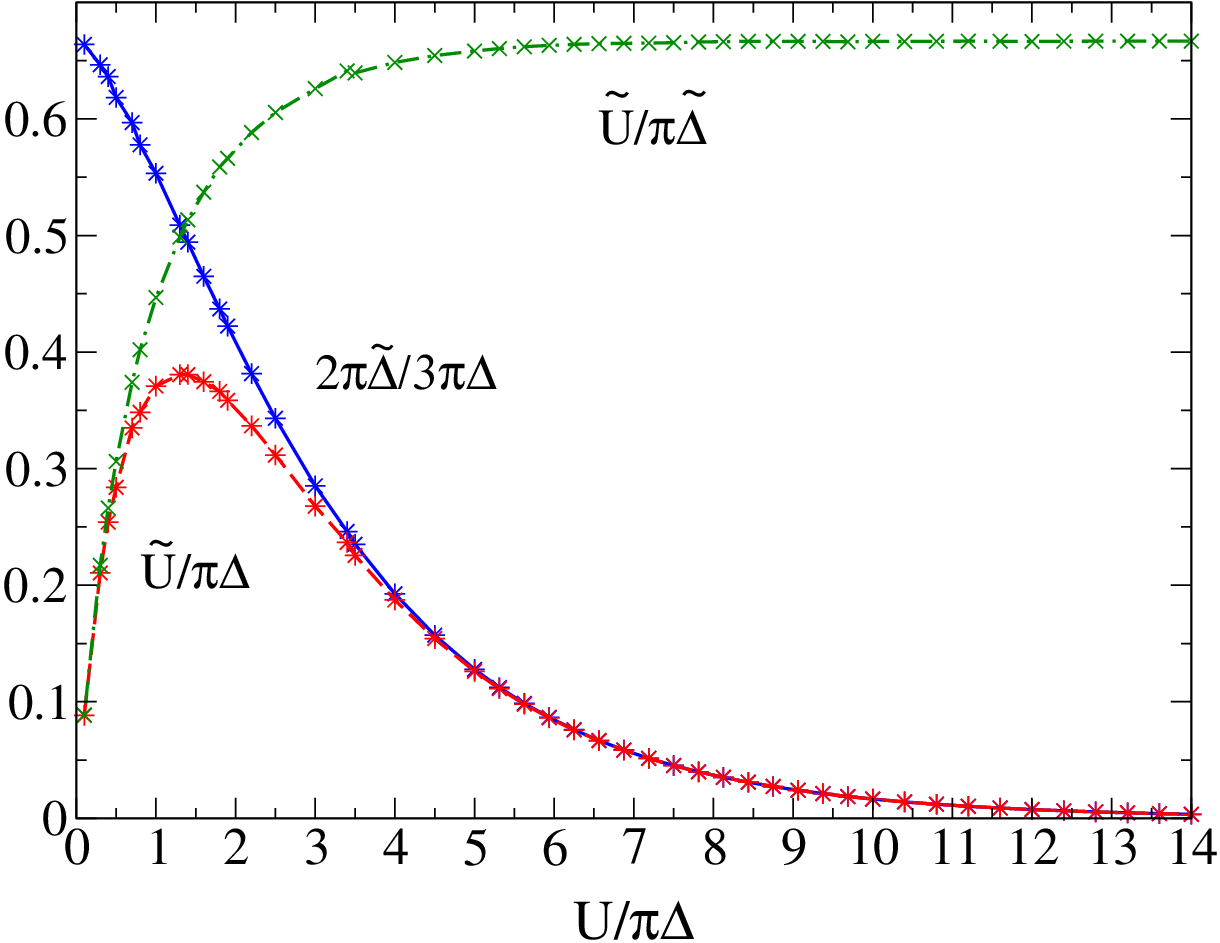
For $n=2$ we expect these relations to be satisfied at the points of integral valence $n_{d}=1,2,3$. In I we have already shown from the NRG calculations for $n=2$ that at the particle-hole symmetric point $n_{d}=2$, the relation $\tilde{U}/\pi\tilde{\Delta}=1/3$ in agreement with Eq. (15). For $n_{d}=1,3$, from Eq. (15) we get the result $\tilde{U}/\pi\tilde{\Delta}=2/3$. In Fig. 2 we plot $2\tilde{\Delta}/3\Delta$, $\tilde{U}/\pi\Delta$, and the ratio $\tilde{U}/\pi\tilde{\Delta}$ for $n_{d}=1$ as a function of $U/\pi\Delta$ for $\pi\Delta=0.01$. It can be seen that there is localization and a single energy scale for $U/\pi\Delta>4.5$, and the ratio $\tilde{U}/\pi\tilde{\Delta}$ asymptotically approaches the value $2/3$. For $U/\pi\Delta=14$ we find $\tilde{U}/\pi\tilde{\Delta}=0.66665$, a very accurate verification of the relation from Eq. (15) for $n_{d}=1$ and $n=2$.

To look at the behavior more generally in the strong correlation regime, we have calculated the renormalized parameters for $U/\pi\Delta=5$, $\Delta=0.01$ over the full range of the occupation number $n_{d}$. The results for $\tilde{\epsilon}_{d}/\pi\Delta$, $\tilde{\Delta}/\Delta$ and $\tilde{U}/\pi\Delta$ are shown in Fig. 3. There are three distinct local minina in $\tilde{\Delta}$ at $n_{d}=2$ and for values of $n_{d}$ slightly greater than 1 and slightly less than 3. This was to be expected, as the regions near integral values of $n_{d}$ for large $U$ correspond to localized Kondo regimes, and the dips in the values of $\tilde{\Delta}$ indicate a narrowing of the quasiparticle density of states at these points. It is an unexpected result, however, that minima away from the particle-hole symmetric point $n_{d}=2$ are not precisely at $n_{d}=1$ and $3$. Also we find in the mixed valence regimes, $1<n_{d}<2$ and $2<n_{d}<3$, there is still some significant renormalization of $\Delta$. For $n_{d}<0.7$ and $n_{d}>3.3$, the values of $\tilde{\Delta}$ rapidly approach the bare value $\Delta$.

In Fig. 4 we give the corresponding results for $\chi_{s}$ and $\chi_{c}$. The enhanced peaks in $\chi_{s}$ in the Kondo regimes near integral values of $n_{d}$ are as expected. It can be seen from Fig. 3 that the values of $\tilde{\Delta}$ at $n_{d}=1,2,3$ are almost the same. The higher value of $\chi_{s}$ at $n_{d}=2$, therefore, is due to the fact that at this point $\tilde{\epsilon}_{d}=0$ giving a higher quasiparticle density of states compared with the peaks near $n_{d}=1$ and $n_{d}=3$. Again we note that the peaks in $\chi_{s}$ near $n_{d}=1$ and $n_{d}=3$ are not precisely at these integer values.

The values of $\chi_{c}$ can be seen to be very small at $n_{d}=2$ and near $n_{d}=1,3$. It is, however, rather small over the whole range, with only modest peaks between the integer values of $n_{d}$. To get more insight into this, we plot $\eta_{s}$ and $\eta_{c}$ for the same set of parameters in Fig. 5. Surprisingly we see that $\eta_{c}$ is very small over the whole range from $n_{d}=1$ to $n_{d}=3$, and not just at the integer values. This indicates that quasiparticle interaction suppresses the charge susceptibility not just for $n_{d}=1,2,3$ but also in the mixed valence regimes $1<n_{d}<2$ and $2<n_{d}<3$. There are slight peaks in $\eta_{c}$ near $n_{d}\sim 1.5$ and $n_{d}\sim 2.5$, but the values are still very small. The Wilson ratio for this model when $n=2$ is equal to $4/3$. It can be seen that $R_{\rm W}\approx 4/3$ over the range $1\leq n_{d}\leq 3$. The fact the $\eta_{c}$ is very small implies that impurity d-electrons are rather localized so that Eq. (15) should be a good approximation over this range. For $n=2$, Eq. (15) becomes

It is also of interest to compare the two integral valence cases, $n_{d}=1$ and $n_{d}=2$. In the Kondo regime for large $U$, the models with $n_{d}=1$ and $n_{d}=2$ can both be mapped onto Coqblin-Schrieffer models of the form,

where the sum over $\nu=1,2,...2n$, and with particle -hole symmetry $J_{\rm eff}=4|V|^{2}/U$. The operators $Y_{\nu,\nu^{\prime}}$ obey the SU(2n) commutation relations,

with $\sum_{\nu}Y_{\nu,\nu}=nI$. Though we are dealing with the model for the same value of $n$, in this case $n=2$, the models for $n_{d}=1$ and $n_{d}=2$, differ in that the operators transform according to different irreducible representations of $SU(4)$. The case with $n_{d}=1$ is the one originally considered by Coqblin and Schrieffer [4], where the representation of the operators $Y_{\nu,\nu^{\prime}}$ is the fundamental representation of the group, which for the SU(4) group has dimension 4. On the other hand for $n_{d}=2$, as we noted in I, the $Y_{\nu,\nu^{\prime}}$ operators correspond to a 6 dimensional irreducible representation of the SU(4) group. This is similar to a Heisenberg model, which can describe physical situations depending on the dimensionality of the irreducible representation used for the spin operators, $2S+1$ for a spin $S$. In the general $n$ channel model with $r$ localized electrons the dimensionality of the irreducible representation of the operators in the Coqblin-Schrieffer model will be $(2n)!/(2n-r)!r!$.

More generally when $n_{d}\leq 1$, and $U/\pi\Delta\gg 1$, the model with $J_{\rm H}=0$ can be related to the $N$-fold degenerate, $U=\infty$, Anderson model which has been applied to rare earth impurities such as Ce and Yb with $N=2n$ [6, 7, 5]. In this application the index $\nu$ corresponds the $z$-component of total angular momentum, orbital plus spin $m_{j}$, with $N=2j+1$, and $j$ is the total angular momentum quantum number. The equation for the total angular momentum susceptibility $\chi_{j}$ for this model is given by

where $g$ is the $g$-factor for coupling to the magnetic field and

while the equation for the charge susceptibility is the same as in Eq. (10) with $2n=N$. The Wilson ratio for the $N$-fold degenerate model ($U=\infty$) is defined as $R_{\rm W}=\pi^{2}\chi_{j}/j(j+1)(g\mu_{\rm B})^{2}\gamma$, giving $R_{\rm W}=\eta_{j}=N/(N-1)$, which is the same as that we have for the SU(2n) model for $N=2n$.

In the localized limit when $U/\pi\Delta$ is large we have only one energy scale which we take to be the Kondo temperature $T_{\rm K}$. For the $N$-fold degenerate, infinite $U$, Anderson model $T_{\rm K}$ is defined such that $\chi_{j}=(g\mu_{\rm B})^{2}j(j+1)/3T_{\rm k}$. This is equivalent to

which we will take as a general definition for $T_{\rm K}$ for the SU(2n) model in the discussion here. It differs from the definition used in I by the factor $(2n-1)/n^{2}$.

On using Eq. (13) for $\tilde{\rho}^{(0)}(0)$, we find

We would expect this formula to apply only at or near the points of integer occupation of the impurity site, $n_{d}=1,2,3$. However, for large $U/\pi\Delta$ we found localization and a Wilson ratio $R_{\rm W}\approx 4/3$ over the complete range $1\leq n_{d}\leq 3$. This means that we can define a Kondo temperature as a function of $n_{d}$ over this range. A plot of $T_{\rm K}$ based on Eq. (22) is given in Fig. 7 for $n=2$ and $U/\pi\Delta=5,10$ ($\Delta=0.01$). There are three dips corresponding to a local minima for $T_{\rm K}$ at $n_{d}=2$ and near $n_{d}=1,3$. For the larger value of $U$ the outer minima move slighter closer towards $n_{d}=1$ and $n_{d}=3$.

We can contrast the quasiparticle density of states in the case of half-filling, $n_{d}=n$, with that for $n_{d}=1$. In the former case, $\tilde{\epsilon}_{d}=0$ and the quasiparticle density of states is symmetrically placed about the Fermi level, and for large $n$, $\tilde{\rho}^{(0)}(\omega)$ takes the approximate form,

For $n_{d}=1$ and $n>1$, on the other hand, the quasiparticle peak is asymmetrically placed about the Fermi level. For large $n$, $\tilde{\rho}^{(0)}(\omega)$ takes the approximate form,

and in the limit $n\to\infty$ collapses to a delta-function at a point $T_{\rm K}$ above the Fermi level. This asymmetry with respect to the Fermi level for $n_{d}=1$, $n>1$, is required by the Friedel sum rule, because if $n_{d}=1$, the quasiparticle density of states must be such that has only a fraction $1/2n$ is filled when integrated up to the Fermi level.

In Fig. 9 we compare the quasiparticle density of states for $n_{d}=1$ and $2$ for $U/\pi\Delta=5$. We see that the peak in the case $n_{d}=1$ is shifted slightly above the Fermi level so that the Friedel sum rule is satisfied in terms of the quasiparticles. This shift has physical consequences. If we ignore the effects of the quasiparticle interactions, which becomes an increasingly good approximation the larger the channel index $n$, we can estimate the low temperature and low magnetic field corrections to the spin susceptibility from a free quasiparticle calculation. The $T^{2}$ and $H^{2}$ correction to the spin susceptibility, as well as the $T^{3}$ correction of the impurity specific heat contribution from this calculation are proportional to

where $\rho^{(0)^{\prime}}(0)$ and $\rho^{(0)^{\prime\prime}}(0)$ are the first and second derivatives of $\rho^{(0)}(\omega)$ evaluated at $\omega=0$. If $|\tilde{\epsilon}_{d}|<\tilde{\Delta}$, which is the case when $\tilde{\epsilon}_{d}=0$, then this coefficient is negative. However, when the quasiparticle density of states becomes asymmetric about the Fermi level such that $|\tilde{\epsilon}_{d}|>\tilde{\Delta}$ it changes sign to become positive. As the susceptibility must eventually decrease at high temperatures and in high magnetic fields, this implies that there must be a peak in $\chi_{s}(T)$ and $\chi_{s}(H)$. Such a peak in found in the exact Bethe ansatz solutions for the $N$-fold degenerate, infinite $U$, Anderson model for $N>3$ [6, 8, 5], and this simple argument provides a qualitative explanation for this behavior. The form of the quasiparticle density of states in the vicinity of the Fermi level also affects the thermopower. The thermopower due to the impurity is proportional to the gradient of the quasiparticle density of states at the Fermi level; it is zero when the quasiparticle density of states is symmetrical about the Fermi level but large when there is narrow peak just above the Fermi level.

It is also possible that shift in the peak in the quasiparticle density of states, which for $n=2$ will be to above the Fermi level for $n_{d}=1$ and below the Fermi level for $n_{d}=3$, may explain why the local minima in renormalized parameters and the peaks in the spin susceptibility do not occur at precisely at $n_{d}=1$ and $n_{d}=3$, but in one case slightly greater than $n_{d}=1$ and in the other slightly less than $n_{d}=3$.

We now consider the case with Hund’s rule coupling away from particle-hole symmetry. In Fig. 10 we show the renormalized parameters $\tilde{\epsilon}_{d}$, $\tilde{\Delta}$, $\tilde{U}$ and $\tilde{J}_{\rm H}$ (in units of $\pi\Delta=0.01$) as a function of the impurity occupation $n_{d}$ for $U/\pi\Delta=4$ and $J_{\rm H}/\pi\Delta=0.15$. The main difference with those seen in Fig. 3 where $J_{\rm H}=0$ is that the minimum at $n_{d}=2$ is much more pronounced than the local minima near $n_{d}=1,3$. The plot of $\eta_{s}$ (=$R_{\rm W}$, Wilson ratio), $\eta_{orb}$ and $\eta_{c}$ in Fig. 11 shows that the quasiparticle interaction from the Hund’s rule coupling induces an enhancement of $\eta_{s}$ and a corresponding reduction of $\eta_{orb}$ in the range between $n_{d}=1$ and $n_{d}=3$. Due to the relatively large value of $U/\pi\Delta$ the value of $\eta_{c}$ is almost completely suppressed between $n_{d}=1$ to $n_{d}=3$ as in the case with $J_{\rm H}=0$.

As $\eta_{c}$ is very small over the range $1\leq n_{d}\leq 3$, we can to a good approximation equate it to zero. From Eq. (11) this gives a relation between the renormalized parameters, which for $n=2$ is

In the discussion of the SU(2n) model, where $J_{\rm H}=0$, this condition left only one independent renormalized parameter, which we could take as the Kondo temperature. However, when $J_{\rm H}\neq 0$, we are left with two renormalized parameters, so we cannot in this case define a Kondo temperature from this equation alone. We see from Fig. 11 that at and very close to $n_{d}=2$ the orbital susceptibility is also suppressed, so equating $\eta_{\rm orb}$ to zero from Eq. (9) we find

At this point we have a single energy scale and can define a Kondo temperature via $\chi_{s}={(g\mu_{\rm B})^{2}S(S+1)/3T_{\rm K}}$ for a spin $S=1$, which is such that

and $\tilde{\epsilon}_{d}=0$ from particle-hole symmetry. At this point the Wilson ratio $R_{\rm W}=\eta_{s}=8/3$, as can seen in Fig. 11. The particle-hole symmetric case with $n_{d}=2$ is discussed more fully in I.

In Fig. 12 we show the renormalized parameters as a function of $n_{d}$ for smaller values of $U$ and $J_{\rm H}$, $U/\pi\Delta=2$ and $J_{\rm H}/\pi\Delta=0.05$. The values of $\tilde{\epsilon}_{d}$, $\tilde{\Delta}$, $\tilde{U}$ are rather similar to the case with $J_{\rm H}=0$ shown in Fig. 3. In this case, in contrast to the previous example, $\tilde{J}_{\rm H}$ has a maximum at $n_{d}=2$ rather than a minimum. For this smaller value of $U$, the renormalized value $\tilde{U}$ is rather flat in most of the range from $n_{d}=1$ to $n_{d}=3$. In Fig. 13 we show the corresponding values for $\eta_{s}$, $\eta_{orb}$ and $\eta_{c}$. It shows that, even for this smaller value of $U$, there is some suppression of the charge susceptibility by the quasiparticle interactions. There is also some enhancement of $\chi_{s}$ and a commensurate reduction in $\eta_{orb}$ as the particle-hole symmetric point $n_{d}=2$ is approached.

In Fig. 14 we show the renormalized parameters with the same value of $J_{\rm H}$ ($J_{\rm H}/\pi\Delta=0.05$) and a larger value of $U$, $U/\pi\Delta=4$. It can be seen that the effect of increasing $U$ is to induce a rather shallow minimum in $\tilde{J}_{\rm H}$ at $n_{d}=2$, and also in $\tilde{U}$. In Fig. 15 we give the corresponding values for $\eta_{s}$, $\eta_{orb}$ and $\eta_{c}$. It can be seen that, despite using the same value of $J_{\rm H}$, $\eta_{s}$ is enhanced and $\eta_{orb}$ is reduced in the central region for the larger value of $U$. This indicates that the enhancement of $\eta_{s}$ does not scale in proportion to $J_{\rm H}/U$, but that $J_{\rm H}$ is more effective in suppressing the orbital fluctuations when the charge fluctuations are suppressed by a larger value of $U$.

In Fig. 16 we compare the quasiparticle density of states at $n_{d}=1$ and $n_{d}=2$ for $U/\pi\Delta=2,4$, $J_{\rm H}=0.05$ and $\pi\Delta=0.01$. It illustrates both the shift in the peak the Kondo resonance to above the Fermi level for $n_{d}=1$, the enhancement of the density of states at the Fermi level, and the narrowing of the resonance for the larger value of $U$.

Finally in Fig. 17 we compare the spin susceptibilities as a function of $n_{d}$ calculated for the three sets of renormalized parameters given in Figs. 10, 12 and 14. The spin susceptibility is considerably enhanced near particle-hole symmetry for the case $J_{\rm H}/\pi\Delta=0.15$ compared with that for $J_{\rm H}/\pi\Delta=0.05$ and the same value of $U$ ($U/\pi\Delta=4$). It also illustrates the more modest enhancement of $\chi_{s}$ for the larger value $U/\pi\Delta=4$ compared with the case for $U/\pi\Delta=2$ and the same value of $J_{\rm H}$ ($J_{\rm H}/\pi\Delta=0.05$).

References

- [1] Y. Nishikawa, D. J. G. Crow, and A. C. Hewson, arXiv:1005.5113, (2010).
- [2] A. C. Hewson, Phys. Rev. Lett. 70, 4007 (1993).
- [3] K. Wilson, Rev. Mod. Phys. 47, 773 (1975).
- [4] B. Coqblin and J. R. Schrieffer, Phys. Rev. 185, 847 (1969).
- [5] A. C. Hewson, The Kondo Problem to Heavy Fermions (Cambridge University Press, Cambridge, 1997).
- [6] E. Orgievetski, A. M. Tsvelik, and P. B. Wiegmann, J. Phys. C 16 (1983).
- [7] P. Schlottmann, Phys. Rep. 181, 1 (1989).
- [8] V. T. Rajan, Phys. Rev. Lett. 51, 308 (1983).