Interference Mitigation Techniques
for Clustered Multicell Joint Decoding Systems
Abstract
Multicell joint processing has originated from information-theoretic principles as a means of reaching the fundamental capacity limits of cellular networks. However, global multicell joint decoding is highly complex and in practice clusters of cooperating Base Stations constitute a more realistic scenario. In this direction, the mitigation of intercluster interference rises as a critical factor towards achieving the promised throughput gains. In this paper, two intercluster interference mitigation techniques are investigated and compared, namely interference alignment and resource division multiple access. The cases of global multicell joint processing and cochannel interference allowance are also considered as an upper and lower bound to the interference alignment scheme respectively. Each case is modelled and analyzed using the per-cell ergodic sum-rate throughput as a figure of merit. In this process, the asymptotic eigenvalue distribution of the channel covariance matrices is analytically derived based on free-probabilistic arguments in order to quantify the sum-rate throughput. Using numerical results, it is established that resource division multiple access is preferable for dense cellular systems, while cochannel interference allowance is advantageous for highly sparse cellular systems. Interference alignment provides superior performance for average to sparse cellular systems on the expense of higher complexity.
Index Terms:
Information theory, Information Rates, Multiuser channels, MIMO systems, Cochannel Interference, Land mobile radio cellular systems, Eigenvalues and eigenfunctions.I Introduction
Currently cellular networks carry the main bulk of wireless traffic and as a result they risk being saturated considering the ever increasing traffic imposed by internet data services. In this context, the academic community in collaboration with industry and standardization bodies have been investigating innovative network architectures and communication techniques which can overcome the interference-limited nature of cellular systems. The paradigm of multicell joint processing has risen as a promising way of overcoming those limitations and has since gained increasing momentum which lead from theoretical research to testbed implementations [1]. Furthermore, the recent inclusion of CoMP (Coordinated Multiple Point) techniques in LTE-Advanced [2] serves as a reinforcement of the latter statement.
Multicell joint processing is based on the idea that signal processing does not take place at individual Base Stations (BSs), but at a central processor which can jointly serve the User Terminals (UTs) of multiple cells through the spatially distributed BSs. It should be noted that the main concept of multicell joint processing is closely connected to the rationale behind Network MIMO and Distributed Antenna Systems (DAS) and those three terms are often utilized interchangeably in the literature. According to the global multicell joint processing, all the BSs of a large cellular system are assumed to be interconnected to a single central processor through an extended backhaul. However, the computational requirements of such a processor and the large investment needed for backhaul links have hindered its realization. On the other hand, clustered multicell joint processing utilizes multiple signal processors in order to form BS clusters of limited size, but this localized cooperation introduces intercluster interference into the system, which has to be mitigated in order to harvest the full potential of multicell joint processing. In this direction, reuse of time or frequency channel resources (resource division multiple access) could provide the necessary spatial separation amongst clusters, an approach which basically mimics the principles of the traditional cellular paradigm only on a cluster scale. Another alternative would be to simply tolerate intercluster signals as cochannel interference, but obviously this scheme becomes problematic in highly dense systems.
Taking all this into account, the current paper considers the uplink of a clustered Multicell Joint Decoding (MJD) system and proposes a new communication strategy for mitigating intercluster interference using Interference Alignment (IA). More specifically, the main contributions herein are:
- 1.
the channel modelling of a clustered MJD system with IA as intercluster interference mitigation technique,
- 2.
the analytical derivation of the ergodic throughput based on free probabilistic arguments in the R-transform domain,
- 3.
the analytical comparison with the upper bound of global MJD, the Resource Division Multiple Access (RDMA) scheme and the lower bound of clustered MJD with Cochannel Interference allowance (CI),
- 4.
the comparison of the derived closed-form expressions with Monte Carlo simulations and the performance evaluation using numerical results.
The remainder of this paper is structured as follows: Section II reviews in detail prior work in the areas of clustered MJD and IA. Section III describes the channel modelling, free probability derivations and throughput results for the following cases: a) global MJD, b) IA, c) RDMA and d) CI. Section IV displays the accuracy of the analysis by comparing to Monte Carlo simulations and evaluates the effect of various system parameters in the throughput performance of clustered MJD. Section V concludes the paper.
I-A Notation
Throughout the formulations of this paper, denotes expectation, denotes the conjugate matrix transpose, denotes the matrix transpose, denotes the Hadamard product and denotes the Kronecker product. The Frobenius norm of a matrix or vector is denoted by and the delta function by . denotes an identity matrix, an matrix of ones, a zero matrix and denotes Gaussian matrix with entries drawn form a distribution. The figure of merit analyzed and compared throughout this paper is the ergodic per-cell sum-rate throughput11 1 The term throughput is used instead of capacity since the described techniques lead to achievable sum-rates except for MJD which leads to MIMO MAC capacity..
II Related Work
II-A Multicell Joint Decoding
This section reviews the literature on MJD systems by describing the evolution of global MJD models and subsequently focusing on clustered MJD approaches.
II-A1 Global MJD
It was almost three decades ago when the paradigm of global MJD was initially proposed in two seminal papers [3, 4], promising large capacity enhancements. The main idea behind global MJD is the existence of a central processor (a.k.a. “hyper-receiver”) which is interconnected to all the BSs through a backhaul of wideband, delayless and error-free links. The central processor is assumed to have perfect Channel State Information (CSI) about all the wireless links of the system. The optimal communication strategy is superposition coding at the UTs and successive interference cancellation at the central processor. As a result, the central processor is able to jointly decode all the UTs of the system, rendering the concept of intercell interference void.
Since then, the initial results were extended and modified by the research community for more practical propagation environments, transmission techniques and backhaul infrastructures in an attempt to more accurately quantify the performance gain. More specifically, it was demonstrated in [5] that Rayleigh fading promotes multiuser diversity which is beneficial for the ergodic capacity performance. Subsequently, realistic path-loss models and user distributions were investigated in [6, 7] providing closed-form ergodic capacity expressions based on the cell size, path loss exponent and geographical distribution of UTs. The beneficial effect of MIMO links was established in [8, 9], where a linear scaling of the ergodic per-cell sum-rate capacity with the number of BS antennas was shown. However, correlation between multiple antennas has an adverse effect as shown in [10], especially when correlation affects the BS-side. Imperfect backhaul connectivity has also a negative effect on the capacity performance as quantified in [11]. MJD has been also considered in combination with DS-CDMA [12], where chips act as multiple dimensions. Finally, linear MMSE filtering [13, 14] followed by single-user decoding has been considered as an alternative to the optimal multiuser decoder which requires computationally-complex successive interference cancellation.
II-A2 Clustered MJD
Clustered MJD is based on forming groups of adjacent BSs (clusters) interconnected to a cluster processor. As a result, it can be seen as an intermediate state between traditional cellular systems () and global MJD (). The advantage of clustered MJD lies on the fact that both the size of the backhaul network and the number of UTs to be jointly processed decrease. The benefit is twofold; firstly, the extent of the backhaul network is reduced and secondly, the computational requirements of MJD (which depend on the number of UTs) are lower. The disadvantage is that the sum-rate capacity performance is degraded by intercluster interference, especially affecting the individual rates of cluster-edge UTs. This impairment can be tackled using a number of techniques as described here. The simplest approach is to just treat it as cochannel interference and evaluate its effect on the system capacity as in [15]. An alternative would be to use RDMA, namely to split the time or frequency resources into orthogonal parts dedicated to cluster-edge cells [16]. This approach eliminates intercluster interference but at the same time limits the available degrees of freedom. In DS-CDMA MJD systems, knowledge of the interfering codebooks has been also used to mitigate intercluster interference [12]. Finally, antenna selection schemes were investigated as a simple way of reducing the number of intercluster interferers [17].
II-B Interference Alignment
This section reviews the basic principles of IA and subsequently describes existing applications of IA on cellular networks.
II-B1 IA Preliminaries
IA has been shown to achieve the degrees of freedom (dofs) for a range of interference channels [18, 19, 20]. Its principle is based on aligning the interference on a signal subspace with respect to the non-intended receiver, so that it can be easily filtered out by sacrificing some signal dimensions. The advantage is that this alignment does not affect the randomness of the signals and the available dimensions with respect to the intended receiver. The disadvantage is that the filtering at the non-intended receiver removes the signal energy in the interference subspace and reduces the achievable rate. The fundamental assumptions which render IA feasible are that there are multiple available dimensions (space, frequency, time or code) and that the transmitter is aware of the CSI towards the non-intended receiver. The exact number of needed dimensions and the precoding vectors to achieve IA are rather cumbersome to compute, but a number of approaches have been presented in the literature towards this end [21, 22, 23].
II-B2 IA and Cellular Networks
IA has been also investigated in the context of cellular networks, showing that it can effectively suppress cochannel interference [24, 23]. More specifically, the downlink of an OFDMA cellular network with clustered BS cooperation is considered in [25], where IA is employed to suppress intracluster interference while intercluster interference has to be tolerated as noise. Using simulations, it is shown therein that even with unit multiplexing gain the throughput performance is increased compared to a frequency reuse scheme, especially for the cluster-centre UTs. In a similar setting, the authors in [26] propose an IA-based resource allocation scheme which jointly optimizes the frequency-domain precoding, subcarrier user selection, and power allocation on the downlink of coordinated multicell OFDMA systems. In addition, authors in [24] consider the uplink of a limited-size cellular system without BS cooperation, showing that the interference-free dofs can be achieved as the number of UTs grows. Employing IA with unit multiplexing gain towards the non-intended BSs, they study the effect of multi-path channels and single-path channels with propagation delay. Furthermore, the concept of decomposable channel is employed to enable a modified scheme called subspace IA, which is able to simultaneously align interference towards multiple non-intended receivers over a multidimensional space. Finally, the effect of limited feedback on cellular IA schemes has been investigated and quantified in [25, 27].
III Channel Model & Throughput Analysis
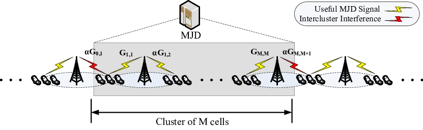
In this paper, the considered system comprises a modified version of Wyner’s linear cellular array [4, 12, 28], which has been used extensively as a tractable model for studying MJD scenarios. In the modified model studied herein, MJD is possible for clusters of adjacent BSs while the focus is on the uplink. Unlike [24, 23], IA is employed herein to mitigate intercluster interference between cluster-edge cells. Let us assume that UTs are positioned between each pair of neighboring BSs with path loss coefficients 1 and respectively (Figure 1). All BSs and UTs are equipped with antennas to enable IA over the multiple spatial dimensions for the clustered UTs. In this setting, four scenarios of intercluster interference are considered, namely global MJD, IA, RDMA and CI. It should be noted that only cluster-edge UTs employ interference mitigation techniques, while UTs in the interior of the cluster use the optimal wideband transmission scheme with superposition coding as in [5]. Successive interference cancellation is employed in each cluster processor in order to recover the UT signals. Furthermore, each cluster processor has full CSI for all the wireless links in its coverage area. The following subsections explain the mode of operation for each approach and describe the analytical derivation of the per-cell sum-rate throughput.
III-A Global Multicell Joint Decoding
In global MJD, a central processor is able to jointly decode the signals received by neighboring clusters and therefore no intercluster interference takes place. In other words, the entire cellular system can be assumed to be comprised of a single extensive cluster. As it can be seen, this case serves as an upper bound to the IA case. The received symbol vector at any random BS can be expressed as follows:
| (1) |
where the vector denotes AWGN with and . The vector denotes the transmitted symbol vector of the th UT group with where is the transmit Signal to Noise Ratio per UT antenna. The channel matrix includes the flat fading coefficients of the th UT group towards the th BS modelled as independent identically distributed (i.i.d.) complex circularly symmetric (c.c.s.) random variables. Similarly, the term represents the received signal at the th BS originating from the UTs of the neighboring cell indexed . The scaling factor models the amount of received intercell interference which depends on the path loss model and the density of the cellular system22 2 For more details on the modelling of the parameter, the reader is referred to [29].. Another intuitive description of the factor is that it models the power imbalance between intra-cell and inter-cell signals.
Assuming a memoryless channel, the system channel model can be written in a vectorial form as follows:
| (2) |
where the aggregate channel matrix has dimensions and can be modelled as:
| (3) |
with being a block-Toeplitz matrix and . In addition, is a Toeplitz matrix structured as follows:
| (4) |
Assuming no CSI at the UTs, the per-cell capacity is given by the MIMO Multiple Access (MAC) channel capacity:
| (5) |
Theorem III.1
In the global MJD case, the per-cell capacity for asymptotically large converges almost surely (a.s.) to the Marčenko-Pastur (MP) law with appropriate scaling [6, 10]:
| (6) |
Proof:
For the sake of completeness and to facilitate latter derivations, an outline of the proof in [6, 10] is provided here. The derivation of this expression is based on an asymptotic analysis in the number of antennas :
| (7) |
where and denote the eigenvalues and the asymptotic eigenvalue probability distribution function (a.e.p.d.f.) of matrix respectively and denotes the Shannon transform of with scalar parameter . It should be noted that denotes the total UT transmit power normalized by the receiver noise power33 3 For the purposes of the analysis the variable is kept finite as the number of antennas grows large, so that the system power does not grow to infinity.. The last step of the derivation is based on unit rank matrices decomposition and analysis on the R-transform domain, as presented in [6, 10]. The scaling factor
| (8) |
is the Frobenius norm of the matrix normalized by the matrix dimensions and
| (9) |
where step follows from [10, Eq.(34)]. ∎
III-B Interference Alignment
In order to evaluate the effect of IA as an intercluster interference mitigation technique, a simple precoding scheme is assumed for the cluster-edge UT groups, inspired by [24]. Let us assume a unit norm reference vector with and
| (10) |
| (11) |
where and represent the received signal vectors at the first and last BS of the cluster respectively. The first UT group has to align its input towards the non-intended BS of the cluster on the left (see Fig. 1), while the th BS has to filter our the aligned interference coming from the th UT group which belongs to the cluster on the right. These two strategies are described in detail in the following subsections:
III-B1 Aligned Interference Filtering
The objective is to suppress the term which represents intercluster interference. It should be noted that UTs of the th cell are assumed to have perfect CSI about the channel coefficients . Let us also assume that and represent the transmitter vector and channel matrix of the th UT in the th group towards the th BS. In this context, the following precoding scheme is employed to align interference:
| (12) |
where is a scaled version of which satisfies the input power constraint . This precoding results in unit multiplexing gain and is by no means the optimal IA scheme, but it serves as a tractable way of evaluating the IA performance. Following this approach, the intercluster interference can be expressed as:
| (13) |
It can be easily seen that interference has been aligned across the reference vector and it can be removed using a zero-forcing filter designed so that is a truncated unitary matrix [19] and . After filtering, the received signal at the th BS can be expressed as:
| (14) |
Assuming that the system operates in high-SNR regime and is therefore interference limited, the effect of the AWGN noise colouring can be ignored, namely .
Lemma III.1
The Shannon transform of the covariance matrix of is equivalent to that of a Gaussian matrix .
Proof:
Using the property , it can be written that:
| (15) |
The truncated unitary matrix has unit singular values and therefore the matrix product has unit eigenvalues and a zero eigenvalue. Applying eigenvalue decomposition on , the left and right eigenvectors can be absorbed by the isotropic Gaussian matrices and respectively, while the zero eigenvalue removes one of the dimensions. Using the definition of Shannon transform [30], eq. (15) yields
| (16) |
∎
Based on this lemma and for the purposes of the analysis, is replaced by in the equivalent channel matrix.
III-B2 Interference Alignment
The th BS has filtered out incoming interference from the cluster on the right (Figure 1), but outgoing intercluster interference should be also aligned to complete the analysis. This affects the first UT group which should align its interference towards the th BS of the cluster on the left (Figure 1). Following the same precoding scheme and using eq. (10)
| (17) |
where represents the fading coefficients of the th UT of the first group towards the th BS of the neighboring cluster on the left. Since the exact eigenvalue distribution of the matrix product is not straightforward to derive, for the purposes of rate analysis it is approximated by a Gaussian vector with unit variance. This approximation implies that IA precoding does not affect the statistics of the equivalent channel towards the intended BS.
III-B3 Equivalent Channel Matrix
To summarize, IA has the following effects on the channel matrix used for the case of global MJD. The intercluster interference originating from the th UT group is filtered out and thus vertical dimensions are lost. During this process, one horizontal dimension of the th BS is also filtered out, since it contains the aligned interference from the th UT group. Finally, the first UT group has to precode in order to align its interference towards the th BS of neighboring cluster and as a result only out of dimensions are preserved. The resulting channel matrix can be described as follows:
| (18) |
where and
| (19) |
with being a matrix44 4 The structure of the first block of originates in the Gaussian approximation of ., being a matrix and being a matrix55 5 The structure of the last block of is based on Lemma III.1..
Since all intercluster interference has been filtered out and the effect of filter has been already incorporated in the structure of , the per-cell throughput in the IA case is still given by the MIMO MAC expression:
| (20) | ||||
Theorem III.2
In the IA case, the per-cell throughput can be derived from the R-transform of the a.e.p.d.f. of matrix .
Proof:
Following an asymptotic analysis where :
| (21) |
The a.e.p.d.f. of is obtained by determining the imaginary part of the Stieltjes transform for real arguments
| (22) |
considering that the Stieltjes transform is derived from the R-transform [31] as follows
| (23) |
∎
Theorem III.3
The R-transform of the a.e.p.d.f. of matrix is given by:
| (24) |
with parameters given by:
and given by theorem A.1.
III-C Resource Division Multiple Access
RDMA entails that the available time or frequency resources are divided into two orthogonal parts assigned to cluster-edge cells in order to eliminate intercluster interference [16, Efficient isolation scheme]. While double the power can be transmitted in each orthogonal part, the available channel resources are cut in half for cluster-edge cells. The channel modelling is similar to the one in global MJD case (eq. (1)), although in this case the throughput is analyzed separately for each orthogonal part and subsequently averaged. Assuming no CSI at the UTs, the per-cell throughput in the RDMA case is given by:
| (26) |
where and denote the capacities when the cluster-edge UTs are active and inactive respectively. When the cluster-edge UTs are active, the cluster processor receives signals from all BSs and the resulting channel matrix is structured as follows:
| (27) |
where the factor is due to the doubling of the transmitted power.
Theorem III.4
In the RDMA case with active cluster-edge UTs, the per-cell throughput can be derived from the R-transform of the a.e.p.d.f. of matrix , where:
| (28) |
When the cluster-edge UTs are inactive, the cluster processor receives signals from BSs and the resulting channel matrix is structured as follows:
| (31) |
Theorem III.5
In the RDMA case with inactive cluster-edge UTs, the per-cell throughput can be derived from the R-transform of the a.e.p.d.f. of matrix , where:
| (32) |
Proof:
Following an asymptotic analysis where :
| (33) |
The rest of this proof follows the steps of Theorem 28. ∎
III-D Cochannel Interference Allowance
CI is considered as a worst case scenario where no signal processing is performed in order to mitigate intercluster interference [32]. As it can be seen, this case serves as a lower bound to the IA case. The channel modelling is identical with the one in global MJD case (eq. (1)), although in this case the cluster-edge UT group contribution is considered as interference. As a result, the interference channel matrix can be expressed as:
| (34) |
Assuming no CSI at the UTs, the per-cell throughput in the CI case is given by:
| (35) |
where denotes the throughput of the interfering UT group normalized by the cluster size:
| (36) |
III-E Degrees of freedom
This section focuses on comparing the degrees of freedom for each of the considered cases. The degrees of freedom determine the number of independent signal dimensions in the high SNR regime and it is also known as prelog or multiplexing gain in the literature. It is a useful metric in cases where interference is the main impairment and AWGN can be considered unimportant.
Theorem III.7
The degrees of freedom per BS antenna for the global MJD, IA, RDMA and CI cases are given by:
| (39) |
Lemma III.2
The following inequalities apply for the dofs of eq. (39):
| (40) |
Remark III.1
It can be observed that only for single UT per cell equipped with two antennas (). For all other cases, . Furthermore, it is worth noting that when the number of UTs and antennas grows to infinity, which entails a multiuser gain. However, in practice the number of served UTs is limited by the number of antennas () which can be supported at the BS- and more importantly at UT-side due to size limitations.
III-F Complexity Considerations
This paragraph discusses the complexity of each scheme in terms of decoding processing and required CSI. In general, the complexity of MJD is exponential with the number of users [33] and full CSI is required at the central processor for all users which are to be decoded. This implies that global MJD is highly complex since all system users have to be processed at a single point. On the other hand, clustering approaches reduce the number of jointly-processed users and as a result complexity. Furthermore, CI is the least complex since no action is taken to mitigate intercluster interference. RDMA has an equivalent receiver complexity with CI but in addition it requires coordination between adjacent clusters in terms of splitting the resources. For example, time division would require inter-cluster synchronization, while frequency division could be even static. Finally, IA is the most complex since CSI towards the non-intended BS is also needed at the transmitter in order to align the interference. Subsequently, additional processing is needed at the receiver side to filter out the aligned interference.
IV Numerical Results
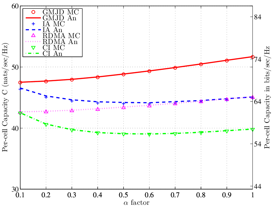
This section presents a number of numerical results in order to illustrate the accuracy of the derived analytical expressions for finite dimensions and evaluate the performance of the aforementioned interference mitigation schemes. In the following figures, points represent values calculated through Monte Carlo simulations, while lines refer to curves evaluated based on the analytical expressions of section III. More specifically, the simulations are performed by generating instances of random Gaussian matrices, each one representing a single fading realization of the system. In addition, the variance profile matrices are constructed deterministically based on the considered factors and used to shape the variance of the i.i.d. c.c.s. elements. Subsequently, the per-cell capacities are evaluated by averaging over the system realizations using: a) eq. (5) for global MJD, b) eq. (10)-(14) and (20) for IA, c) eq. (26) for RDMA, d) eq. (35),(36) for CI. In parallel, the analytical curves are evaluated based on: a) theorem III.1 for global MJD, b) theorems III.2 and III.3 for IA, c) theorems 28 and 32 for RDMA, d) theorems III.1 and 37 for CI. Table I presents an overview of the parameter values and ranges used for producing the numerical results of the figures.
Firstly, figure 2 depicts the per-cell throughput versus the cluster size for medium factors. It should be noted that the factor combines the effects of cell size and path loss exponent as explained in [29]. As expected the performance of global MJD does not depend on the cluster size, since it is supposed to be infinite. For all interference mitigation techniques, it can be seen that the penalty due to the clustering diminishes as the cluster size increases. Similar conclusions can be derived by plotting the degrees of freedom versus the cluster size (figure 3). In addition, it can be observed that the IA dofs approach the global MJD dofs as the number of UTs and antennas increases. Subsequently, Figure 4 depicts the per-cell throughput versus the factor. For high factors, RDMA performance converges to IA, whereas for low factors RDMA performance degrades and touched the CI curve. It should be also noted that while the performance of global MJD and RDMA increase monotonically with , the performances of IA and cochannel interference degrade for medium factors. Finally, figure 5 depicts the per-cell throughput versus the number of UTs per cell . It should be noted that the number of antennas per UT scale jointly with . Based on this observation, a superlinear scaling of the performance can be observed, resulting primarily from the increase of spatial dimensions (more antennas) and secondarily from the increase of the system power (more UTs). As it can be seen, the slope of the linear scaling is affected by the selected interference mitigation technique.
V Conclusion
In this paper, various techniques for mitigating intercluster interference in clustered MJD were investigated. The case of global MJD was initially considered as an upper bound, serving in evaluating the degradation due to intercluster interference. Subsequently, the IA scheme was analyzed by deriving the asymptotic eigenvalue distribution of the channel covariance matrix using free-probabilistic arguments. In addition, the RDMA scheme was studied as a low complexity method for mitigating intercluster interference. Finally, the CI was considered as a worst-case scenario where no interference mitigation techniques is employed. Based on these investigations it was established, that for dense cellular systems the RDMA scheme should be used as the best compromise between complexity and performance. For average to sparse cellular systems which is the usual regime in macrocell deployments, IA should be employed when the additional complexity and availability of CSI at transmitter side can be afforded. Alternatively, CI could be preferred especially for highly sparse cellular systems.
Appendix A Proof of Theorem
Theorem A.1
Let be the concatenation of the variance-profiled Gaussian matrix and a number of zero columns. Let also be the ratio of non-zero to total columns of , be the ratio of horizontal to vertical dimensions of and the Frobenius norm of normalized by the matrix dimensions. The R-transform of is given by:
| (41) |
Proof:
Let be a variance-profiled Gaussian matrix with and . According to [10], the R-transform of is given by:
| (42) |
Using eq. (23), the Stieltjes transform of can be expressed as:
| (43) |
Matrix has identical eigenvalues to plus a number of zero eigevalues with defined as the ratio of non-zero eigenvalues over the total number of eigenvalues. As a result, the a.e.p.d.f. of can be written as:
| (44) |
Using the definition of the Stieltjes transform [30]:
| (45) |
and employing eq. (23), the proof is complete. ∎
References
- [1] EASY-C, “Enablers of Ambient Services and Systems,” http://www.easy-c.de/, 2010.
- [2] 3GPP. (2010) FDD RIT component of SRIT LTE Release 10 & beyond (LTE-Advanced) (source: RP-090745). [Online]. Available: http://www.3gpp.org/ftp/tsg_ran/TSG_RAN/TSGR_45/Documents/RP-090739.zip
- [3] S. V. Hanly and P. A. Whiting, “Information-theoretic capacity of multi-receiver networks,” Telecommun. Syst., vol. 1, pp. 1–42, 1993.
- [4] A. Wyner, “Shannon-theoretic approach to a Gaussian cellular multiple-access channel,” IEEE Trans. Inf. Theory, vol. 40, no. 6, pp. 1713–1727, Nov 1994.
- [5] O. Somekh and S. Shamai, “Shannon-theoretic approach to a Gaussian cellular multiple-access channel with fading,” IEEE Trans. Inf. Theory, vol. 46, no. 4, pp. 1401–1425, Jul 2000.
- [6] S. Chatzinotas, M. Imran, and C. Tzaras, “On the capacity of variable density cellular systems under multicell decoding,” IEEE Commun. Lett., vol. 12, no. 7, pp. 496 – 498, Jul 2008.
- [7] S. Chatzinotas, M. A. Imran, and C. Tzaras, “Optimal information theoretic capacity of the planar cellular uplink channel,” in IEEE 9th Workshop on Signal Processing Advances in Wireless Communications (SPAWC’08), Pernambuco, Brazil, Jul 2008, pp. 196–200.
- [8] D. Aktas, M. Bacha, J. Evans, and S. Hanly, “Scaling results on the sum capacity of cellular networks with MIMO links,” IEEE Trans. Inf. Theory, vol. 52, no. 7, pp. 3264–3274, July 2006.
- [9] S. Chatzinotas, M. A. Imran, and C. Tzaras, “Uplink capacity of MIMO cellular systems with multicell processing,” in IEEE International Symposium on Wireless Communication Systems (ISWCS’08), Reykjavik, Iceland, Oct 2008, pp. 453–457.
- [10] S. Chatzinotas, M. Imran, and R. Hoshyar, “On the multicell processing capacity of the cellular MIMO uplink channel in correlated Rayleigh fading environment,” IEEE Trans. Wireless Commun., vol. 8, no. 7, pp. 3704–3715, July 2009.
- [11] O. Simeone, O. Somekh, H. Poor, and S. Shamai, “Distributed MIMO in multi-cell wireless systems via finite-capacity links,” in Communications, Control and Signal Processing, 2008. ISCCSP 2008. 3rd International Symposium on, March 2008, pp. 203–206.
- [12] O. Somekh, B. Zaidel, and S. Shamai, “Spectral efficiency of joint multiple cell-site processors for randomly spread DS-CDMA systems,” IEEE Trans. Inf. Theory, vol. 53, no. 7, pp. 2625–2637, July 2007.
- [13] B. L. Ng, J. Evans, and S. Hanly, “On the capacity of cellular networks with global LMMSE receiver,” in IEEE International Conference on Communications, 2007. ICC ’07., June 2007, pp. 870–876.
- [14] S. Chatzinotas, R. H. M.A. Imran, and B. Ottersten, “Multicell LMMSE filtering capacity under correlated multiple BS antennas,” in IEEE 72nd Vehicular Technology Conference (VTC’10-Fall), Ottawa, Canada, Sep 2010.
- [15] S. Chatzinotas and B. Ottersten, “Free probability based capacity calculation of multiantenna Gaussian fading channels with cochannel interference,” IEEE Trans. Wireless Commun., 2010, submitted.
- [16] E. Katranaras, M. Imran, and R. Hoshyar, “Sum rate of linear cellular systems with clustered joint processing,” in Vehicular Technology Conference, 2009. VTC Spring 2009. IEEE 69th, 26-29 2009, pp. 1 –5.
- [17] W. Choi and J. Andrews, “Downlink performance and capacity of distributed antenna systems in a multicell environment,” IEEE Trans. Wireless Commun., vol. 6, no. 1, pp. 69–73, Jan 2007.
- [18] V. Cadambe and S. Jafar, “Interference alignment and degrees of freedom of the k -user interference channel,” IEEE Trans. Inf. Theory, vol. 54, no. 8, pp. 3425 –3441, aug. 2008.
- [19] ——, “Interference alignment and the degrees of freedom of wireless X networks,” IEEE Trans. Inf. Theory, vol. 55, no. 9, pp. 3893 –3908, sept. 2009.
- [20] S. Jafar and S. Shamai, “Degrees of freedom region of the MIMO X channel,” IEEE Trans. Inf. Theory, vol. 54, no. 1, pp. 151 –170, Jan 2008.
- [21] K. Gomadam, V. Cadambe, and S. Jafar, “Approaching the capacity of wireless networks through distributed interference alignment,” in Global Telecommunications Conference, 2008. IEEE GLOBECOM 2008. IEEE, Nov 2008, pp. 1 –6.
- [22] C. M. Yetis, T. Gou, S. A. Jafar, and A. H. Kayran, “On feasibility of interference alignment in MIMO interference networks,” IEEE Trans. Signal Processing, vol. 58, no. 9, pp. 4771 – 4782, 2010.
- [23] R. Tresch, M. Guillaud, and E. Riegler, “On the achievability of interference alignment in the K-user constant MIMO interference channel,” in Statistical Signal Processing, 2009. SSP ’09. IEEE/SP 15th Workshop on, Aug 2009, pp. 277 –280.
- [24] C. Suh and D. Tse, “Interference alignment for cellular networks,” in Communication, Control, and Computing, 2008 46th Annual Allerton Conference on, 23-26 2008, pp. 1037 –1044.
- [25] R. Tresch and M. Guillaud, “Cellular interference alignment with imperfect channel knowledge,” in Communications Workshops, 2009. ICC Workshops 2009. IEEE International Conference on, Jun 2009, pp. 1 –5.
- [26] B. Da and R. Zhang, “Exploiting interference alignment in multi-cell cooperative OFDMA resource allocation,” in Submitted to GlobeComm 2011, 2011. [Online]. Available: http://arxiv.org/abs/1103.3093
- [27] N. Lee, W. Shin, and B. Clerckx, “Interference alignment with limited feedback on two-cell interfering two-user MIMO-MAC,” in Submitted to ICC 2011, Oct 2010. [Online]. Available: http://arxiv.org/abs/1010.0933
- [28] O. Somekh, O. Simeone, Y. Bar-Ness, A. M. Haimovich, U. Spagnolini, and S. S. (Shitz), Distributed Antenna Systems: Open Architecture for Future Wireless Communications. Auerbach Publications, CRC Press, May 2007, ch. An information theoretic view of distributed antenna processing in cellular systems.
- [29] S. Chatzinotas, M. Imran, and C. Tzaras, Cooperative Wireless Communications. Auerbach Publications, Taylor & Francis Group, 2009, ch. Capacity Limits in Cooperative Cellular Systems.
- [30] A. M. Tulino and S. Verdú, “Random matrix theory and wireless communications,” Commun. Inf. Theory, vol. 1, no. 1, pp. 1–182, 2004.
- [31] N. Raj Rao and A. Edelman, “The polynomial method for random matrices,” Foundations of Computational Mathematics, 2007.
- [32] S. Chatzinotas and B. E. Ottersten, “Free probability based capacity calculation of multiantenna Gaussian fading channels with cochannel interference,” CoRR, vol. abs/1007.2119, 2010.
- [33] S. Verdú, Multiuser Detection. UK: Cambridge University Press, 1998.