Systematic perturbation approach for a dynamical scaling law in a kinetically constrained spin model

Recently, soft materials such as colloidal and granular systems have attracted considerable interest owing to their rich behaviours. For instance, such systems can be in a supercooled state under conditions of low temperatures and high densities [1]. Under such conditions, a characteristic time acts as a function of system parameters such as temperature or density, and often obeys a non-Arrhenius law, which substantially influences the properties of the materials. Understanding the mechanism of such anomalous dynamical behaviours in many-body systems is important in the field of statistical physics.

Kinetically constrained spin model (KCSM) is a simple model that follows the non-Arrhenius law [2, 3, 4]. Thus far, it has been rigorously proved that the characteristic times in some kinds of KCSM on finite-dimensional lattices show super-Arrhenius type and Vogel-Fulcher type behaviours [5, 6]. Furthermore, in the case of a KCSM on a Bethe lattice, another non-Arrhenius type behaviour of a characteristic time has been found by Monte Carlo simulations [7]. From a static aspect, this non-Arrhenius type behaviour is due to a nonergodic transition corresponding to $k$-core percolation; this transition is not a thermodynamic phase transition. Concretely, at this percolation point, the characteristic time diverges with a power law (non-Arrhenius law); this divergence is supposedly controlled by a mode-coupling equation [7].

The above mentioned mode-coupling equations are also believed to be related with the anomalous dynamical behaviours of colloidal or granular systems. A related conjecture is that a finite-dimensional system mimics a nonergodic transition described by a mode-coupling equation in a mean field sense although it is not a true nonergodic transition but a strong finite-size effect [1]. In the case of KCSM, it has been rigorously proved that the nonergodic transition observed specifically in a KCSM on a Bethe lattice does not occur in the model on a finite dimensional lattice although there are the strong finite-size effects arising from the nonergodic transition on the Bethe lattice [8, 9].

This leads us to consider whether the mechanisms of the appearance of such strong finite-size effects for different finite-dimensional systems have common features. In order to resolve this problem, it is necessary to find a relationship between KCSM and mode-coupling equations. However, the mode-coupling equation describing the nonergodic transition has not been derived yet for KCSM on Bethe lattices: there have been some related studies on the derivations of mode-coupling equations for KCSM [10, 11, 12, 13, 14].

In this paper, as a preliminary step to understand such a relationship, we attempt to clarify the dynamical aspect of the universality class of the nonergodic transition observed in Fredrickson-Andersen model (a KCSM) on a Bethe lattice. Concretely, we derive approximately dynamical systems from this model using a perturbation analysis which provides exact final states as stationary solutions above the nonergodic transition. We find that the universal class of the nonergodic transition cannot be captured by each dynamical systems even at any order by itself. Nevertheless, we find that the differences between the time-dependent solutions of the derived dynamical systems and the results obtained by Monte Carlo (MC) simulations are systematically reduced on a perturbation series. Furthermore, we find that this systematic perturbation analysis clarifies the existence of a dynamical scaling law, which provides a implication for a universal relation between a size scale and a time scale near the nonergodic transition.

Let us consider a regular random graph consisting of $N\in\mathbb{N}$ sites, each of which connects to $c\in\mathbb{N}$ sites chosen randomly, where $\mathbb{N}$ is the set of natural numbers. Then ${\rm G}(c,N)$ is defined as a set of such regular random graphs. For the spin variable $\sigma_{i}\in\{-1,1\}$ defined on each site $i\in\{1,\cdots,N\}$ in a graph $\mathcal{G}\in{\rm G}(c,N)$, the Hamiltonian we consider is

where we express ${\boldsymbol{\sigma}}\equiv(\sigma_{i})_{i=1}^{N}$ collectively. Here, as a preliminary step to define the dynamics of the system, let us consider a transition rate $r({\boldsymbol{\sigma}},F_{i}{\boldsymbol{\sigma}})$ from ${\boldsymbol{\sigma}}$ to $F_{i}{\boldsymbol{\sigma}}$, which satisfies the detailed balance condition. Here, $F_{i}$ is the spin flip operator such that $F_{i}{\boldsymbol{\sigma}}=(\sigma_{1},\cdots,-\sigma_{i},\cdots,\sigma_{N})$. Let $B_{i}$ be a set of sites connected to site $i$. Next, we consider the following dynamical rule. If the number of upward spins on the sites in set $B_{i}$ are more than or equal to $k\in\mathbb{N}$, the spin on site $i$ does not flip absolutely; otherwise, the spin on site $i$ flips at a transition rate $r({\boldsymbol{\sigma}},F_{i}{\boldsymbol{\sigma}})$. In other words, under this rule, the transition rate $T({\boldsymbol{\sigma}}\to F_{i}{\boldsymbol{\sigma}})$ from ${\boldsymbol{\sigma}}$ to $F_{i}{\boldsymbol{\sigma}}$ is expressed by $r({\boldsymbol{\sigma}},F_{i}{\boldsymbol{\sigma}})\Theta(2k-c-\sum_{j\in B_{i}}\sigma_{j})$, where $\Theta(x)=1$ for $x>0$, otherwise $0$. We define the situation of a spin $\sigma_{i}$ with $\Theta(2k-c-\sum_{j\in B_{i}}\sigma_{j})=0$ as ‘kinetically constrained’ or simply ‘constrained’. The master equation for the probability $P({\boldsymbol{\sigma}},t)$ that spin configuration at time $t$ is ${\boldsymbol{\sigma}}$ is

In this paper, we consider the case

Under this constrained dynamical rule, it may be confirmed that the canonical distribution is a stationary distribution. Further, in equilibrium, the magnetization per site is $m_{\rm eq}(T)=\tanh(1/2T)$, and the energy density is $-\tanh(1/2T)/2$. Therefore, there are no thermodynamic phase transitions in the system. In this paper, MC simulations are performed by the following rule. First, a site $i$ is randomly chosen. Next, the spin on site $i$ flips with the probability $T({\boldsymbol{\sigma}}\to F_{i}{\boldsymbol{\sigma}})$. This step is repeated and time $t=1$ is defined by $N$ repeated steps. It is plausible that in the thermodynamic limit, this MC simulation is the same as the dynamics of the system described by equation (2).

Here, we briefly review the static aspect of a nonergodic transition in the system caused by the constrained dynamics, which is discussed in the previous study [7]. Suppose that a spin $\sigma_{i}$ is constrained. If this constraint is permanent, we define the situation of a spin $\sigma_{i}$ as ‘frozen’. Here, let us consider a Cayley tree, which has the same local structures as those of the random graph, ignoring the effects of the loop length $O(\log N)$. Let $g\in\{1,2,\cdots,g_{\rm max}\}$ be a generation of a Cayley tree where $g=1$ is assigned to the root. Let us consider the probability $Q_{g}$ that a spin at the $g$-th generation obtained under equilibrium conditions dependent on $T$ is frozen and upward without considering the state of spin at the $(g-1)$-th generation. From the tree structure of the graph, we can obtain the relation

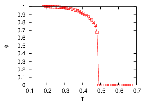
where $p(T)\equiv 1/(1+\exp(-1/T))$. It should be noted that by solving recursion equation (2) for given values of $Q_{g_{\rm max}}$, $Q_{g}$ for $g\ll g_{\rm max}$ becomes a solution $Q(h)$ satisfying $Q(T)=F(Q(T))$. When $c=4$ and $k=3$, $Q(T)$ is zero for sufficiently high temperatures. However, when the temperature is decreased, $Q(T)$ suddenly can take a finite value at finite temperature $T_{\rm c}=0.480898$, as shown in the left-hand side of figure 1. This singular point is $k$-core percolation point, below which the system is nonergodic. Using the quantity $Q(T)$, the fraction $\phi$ of frozen spins is described as

where $Q^{\prime}(T)=p(T)\sum_{n=k}^{c-1}\left(\begin{array}[]{c}c-1\\ n\end{array}\right)Q(T)^{n}(1-Q(T))^{c-1-n}$. In this model, it has been known that for $2<k<c$, this type of nonergodic transition occurs at $T=T_{c}$ with $0<T_{c}<\infty$. For $k=c$, $T_{\rm c}$ is zero, and for $k\leq 2$, $T_{\rm c}$ is $\infty$. The schematic phase diagram is shown in the right-hand side of figure 1.

Although master equation (2) provides the complete information about the system, it is very difficult to extract useful information of the system from (2) because the system has $2^{N}$ states, which is quite a large number when $N$ is large. To avoid this difficulty, we consider describing the system by $N_{\rm eff}\in\mathbb{N}$ number of variables and derive approximately a dynamical system closed by the set of the variables, where $N_{\rm eff}$ remains finite when $N\to\infty$. For simplicity, we consider the relaxation behaviours of the system for the initial condition $\hat{m}(0)=-1$ where $\hat{m}(t)\equiv\sum_{i=1}^{N}\sigma_{i}/N$. It should be noted that the spin configuration for $\hat{m}(0)=-1$ has no constrained spins. In the following analysis, we fix a graph $\mathcal{G}\in{\rm G}(c,N)$ for sufficiently large $N$ without considering ensembles for ${\rm G}(c,N)$. In other words, the following analysis can be applicable to almost all graphs $\mathcal{G}\in{\rm G}(c,N)$ in the thermodynamic limit.

As a first step to derive an effective dynamical system, let $P_{i}(\sigma;t)$ be the probability that $\sigma_{i}$ takes $\sigma$ at time $t$ and $P_{i}((\sigma_{j}^{\prime})|\sigma^{\prime};t)$ be the probability that the spin configuration on the sites in set $B_{i}$ is $(\sigma_{j}^{\prime})_{j\in B_{i}}$ provided that $\sigma_{i}$ takes $\sigma^{\prime}$ at time $t$. Then, we have the following exact evolution equation.

where we define $r_{\sigma}\equiv\min(1,\exp(-\sigma/T))$. Here, we assume that the value of $P_{i}((\sigma_{j}^{\prime})|\sigma)$ does not depend on the chosen site $i$. This assumption may be plausible because at least, in this case, inhomogeneous properties of the system arising from the effects of loops of the random graph $\mathcal{G}$ may be negligible in the thermodynamic limit. This assumption corresponds to the assumption that $P_{i}((\sigma_{j}^{\prime})|\sigma)$ is the same as the conditional probability $P((\sigma_{j}^{\prime})|\sigma;t)$ that if a site with spin variable $\sigma$ is randomly chosen, the spin configuration of its nearest neighbor sites is $(\sigma_{j}^{\prime})$. With this assumption, equation (14) is rewritten as

where $B_{\sigma}$ is a set of sites connected to a site with spin variable $\sigma$ and $\rho_{\sigma}\equiv\sum_{i=1}^{N}P_{i}(\sigma)/N$. It is plausible that $\rho_{\sigma}$ is identical to $\sum_{i}\delta(\sigma-\sigma_{i})/N$ in the thermodynamic limit $N\to\infty$. That is, the magnetization is expressed as $m(t)=\sum_{\sigma}\sigma\rho_{\sigma}(t)$.

Next, we use the approximation that the spin variables on individual sites are independent of each other, which is exact for equilibrium spin configurations. That is, we rewrite $P((\sigma_{j}^{\prime})|\sigma;t)$ as

Further, we can obtain a simpler expression as follows.

where we define $f\equiv c-k+1$. Equations (14), (16), and (3) lead to a closed dynamical system in terms of ${\boldsymbol{\rho}}^{(0)}\equiv(\rho_{\sigma})_{\sigma}$,

It should be noted that stationary solutions of dynamical system (20) provide the exact final states above the nonergodic transition point. However, behaviours of the system at intermediate time scales are very different from the MC simulations, as seen in figure 2. This means that approximation (16) fails to capture heterogeneous spin configurations responsible for the dynamics in intermediate time scales. In this paper, we use the fourth-order Runge-Kutta method for obtaining solutions of dynamical systems with the time discretization $dt=10^{-2}$.

Here, let us consider a persistent time $\tau_{p}(i)$ of a site $i$, which is the time span for a spin to flip at site $i$. Next, let us focus on the target site $i$ in the set ${\rm C}_{i}$ of sites on which constrained spins are connected to each other. Clearly, $\tau_{p}(i)$ strongly depends on the entire spin configuration of sites in set ${\rm C}_{i}$ because the spins from a edge site in set ${\rm C}_{i}$ must be flipped in order to flip the target spin $\sigma_{i}$. Furthermore, the spin configuration on the sites in set ${\rm C}_{i}$ is heterogeneous in terms of the spin direction if it is prepared from the equilibrium spin configurations. This suggests that in order to detect growing relaxation times of the system with respect to the persistent time, it is necessary to obtain information of the heterogeneous configurations of the connected constrained spins.

From the results in the previous section, heterogeneous spin configurations seem to play important roles in the growing relaxation times of the system. Therefore, in order to continue our analysis, we attempt to apply the information of the surrounding spin configurations of a target site perturbatively to effective variables by increasing the value of $N_{\rm eff}$. Such a method has been previously applied to some systems and was successful in determining some nontrivial dynamical properties [15, 16].

References

- [1] Cavagna A. 2009 Phys. Rep. 476 51.
- [2] Fredrickson G. H. and Andersen H. C. 1984 Phys. Rev. Lett. 53 1244.
- [3] Kob W. and Andersen H. C. 1993 Phys. Rev. Lett.. 48 4364.
- [4] Ritort F. and Sollich P. 2003 Adv. Phys. 52 219.
- [5] Toninelli C. and Biroli G. 2007 J. Stat. Phys. 130 83.
- [6] Cancrini N., Martinelli F., Roberto C. and Toninelli C. 2007 J. Stat. M L03001.
- [7] Sellitto M., Biroli G. and Toninelli C. 2005 Europhys. Lett. 69 496.
- [8] Toninelli C., Biroli G. and Fisher D. 2004 Phys. Rev. Lett. 18 185504.
- [9] Toninelli C., Biroli G. and Fisher D. 2005 J. Stat. Phys. 120 167.
- [10] Eisinger S. and Jäckle J. 1993 J. Stat. Phys. 73 643.
- [11] Kawasaki K. 1995 Physica A 215 61.
- [12] Pitts S., Young T. and Andersen H. C. 2000 J. Chem. Phys. 113 8671.
- [13] Pitts S. and Andersen H. C. 2001 J. Chem. Phys. 114 1101.
- [14] Szamel G. 2004 J. Chem. Phys. 2004 3355.
- [15] Semerjian G. and Weigt M. 2004 J. Phys. A 37 5525.
- [16] Ohta H. 2010 J. Phys. A 43 395003.
- [17] Semerjian G. 2007 J. Stat. Phys. 130 251.
- [18] Montanari A. and Semerjian G. unpublished note.
- [19] Montanari A. and Semerjian G. 2004 Phys. Rev. Lett. 94 247201.
- [20] Farrow C. L., Shukla P. and Duxbury P. M. 2007 J. Phys. A 40 F581.
- [21] Farrow C. L., Duxbury P. M. and Moukarzel C. 2005 Phys. Rev. E 72 066109.
- [22] Iwata M. and Sasa S. 2009 J. Phys. A 42 075005.
- [23] Dhar D., Shukla P. and Sethna J. P. 1997 J Phys A: Math. Gen. J. Phys. A 30 5259.
- [24] Sabhabandit S., Dhar D. and Shukla P. 2002 Phys. Rev. Lett. 88 197202.
- [25] Ohta H. and Sasa S. 2010 Europhys. Lett. 90 27008.
- [26] Schwarz J. M., Liu A. J. and Chayes L. Q. 2006 Europhys. Lett. 73 560.
- [27] Jeng M. and Schwarz J. M. 2010 Phys. Rev. E 81 011134.