Adapting to the Shifting Intent of Search QueriesThanks: This is the full version of a paper in NIPS 2009.
Abstract
Search engines today present results that are often oblivious to abrupt shifts in intent. For example, the query ‘independence day’ usually refers to a US holiday, but the intent of this query abruptly changed during the release of a major film by that name. While no studies exactly quantify the magnitude of intent-shifting traffic, studies suggest that news events, seasonal topics, pop culture, etc account for 50% of all search queries. This paper shows that the signals a search engine receives can be used to both determine that a shift in intent has happened, as well as find a result that is now more relevant. We present a meta-algorithm that marries a classifier with a bandit algorithm to achieve regret that depends logarithmically on the number of query impressions, under certain assumptions. We provide strong evidence that this regret is close to the best achievable. Finally, via a series of experiments, we demonstrate that our algorithm outperforms prior approaches, particularly as the amount of intent-shifting traffic increases.
1 Introduction
Search engines typically use a ranking function to order results. The function scores a document by the extent to which it matches the query, and documents are ordered according to this score. Usually, this function is fixed in the sense that it does not change from one query to another and also does not change over time.
Intuitively, a query is “intent-shifting” if the most desired search result(s) change over time. More concretely, a query’s intent has shifted if the click distribution over search results at some time differs from the click distribution at a later time. For the query ‘tomato’ on the heels of a tomato salmonella outbreak, the probability a user clicks on a news story describing the outbreak increases while the probability a user clicks on the Wikipedia entry for tomatoes rapidly decreases. There are studies that suggest that queries likely to be intent-shifting — such as pop culture, news events, trends, and seasonal topics queries — constitute roughly half of the search queries that a search engine receives [10].
The goal of this paper is to devise an algorithm that quickly adapts search results to shifts in user intent. Ideally, for every query and every point in time, we would like to display the search result that users are most likely to click. Since traditional ranking features like PageRank [4] change slowly over time, and may be misleading if user intent has shifted very recently, we want to use just the observed click behavior of users to decide which search results to display.
There are many signals a search engine can use to detect when the intent of a query shifts. Query features such as as volume, abandonment rate, reformulation rate, occurrence in news articles, and the age of matching documents can all be used to build a classifier which, given a query, determines whether the intent has shifted. We refer to these features as the context, and an occassion when a shift in intent occurs as an event.
One major challenge in building an event classifier is obtaining training data. For most query and date combinations (e.g. ‘tomato, 06/09/2008’), it will be difficult even for a human labeler to recall in hindsight whether an event related to the query occurred on that date. In this paper, we propose a novel solution that learns from unlabeled contexts and user click activity.
Contributions. We describe a new algorithm that leverages the information contained in contexts, provided that such information is sufficiently rich. Specifically, we assume that there exists a deterministic oracle (unknown to the algorithm) which inputs the context and outputs a correct binary prediction of whether an event has occurred in the current round. To simulate such an oracle, we use a classification algorithm. However, we do not assume that we have a priori labeled samples to train such a classifier. Instead, we generate the labels ourselves.
Our algorithm is in fact a meta-algorithm that combines a bandit algorithm designed for the event-free setting with an online classification algorithm. The classifier uses the contexts to predict when events occur, and the bandit algorithm “starts over” on positive predictions. The bandit algorithm provides feedback to the classifier by checking, soon after each of the classifier’s positive predictions, whether the optimal search result actually changed. In such a setup, one needs to overcome several technical hurdles, e.g. ensure that the feedback is not “contaminated” by events in the past and in the near future. We design the whole triad — the bandit algorithm, the classifier, and the meta-algorithm — so as to obtain strong provable guarantees. Our bandit subroutine — a novel version of algorithm ucb1 from [2] which additionally provides high-confidence estimates on the suboptimality of arms — may be of independent interest.
For suitable choices of the bandit and classifier subroutines, the regret incurred by our meta-algorithm is (under certain mild assumptions) at most , where is the number of events, is a certain measure of the complexity of the concept class used by the classifier, is the number of relevant search results,11 1 In practice, the arms can be restricted to, say, the top ten results that match the query. is the “minimum suboptimality” of any search result (defined formally in Section 3), and is the total number of impressions. This regret bound has a very weak dependence on , which is highly desirable for search engines that receive much traffic.
The context turns out to be crucial for achieving logarithmic dependence on . Indeed, we show that any bandit algorithm that ignores context suffers regret , even when there is only one event. Unlike many lower bounds for bandit problems, our lower bound holds even when is a constant independent of . We also show that assuming a logarithmic dependence on , the dependence on and is essentially optimal.
For empirical evaluation, we ideally need access to the traffic of a real search engine so that search results can be adapted based on real-time click activity. Since we did not have access to live traffic, we instead conduct a series of synthetic experiments. The experiments show that if there are no events then the well-studied ucb1 algorithm [2] performs the best. However, when many different queries experience events, the performance of our algorithm significantly outperforms prior methods.
2 Related Work
While there has been a substantial amount of work on ranking algorithms [11, 5, 13, 8, 6], all of these results assume that there is a fixed ranking function to learn, not one that shifts over time. Online bandit algorithms (see [7] for background) have been considered in the context of ranking. For instance, Radlinski et al [20] showed how to compose several instantiations of a bandit algorithm to produce a ranked list of search results. Pandey et al [19] showed that bandit algorithms can be effective in serving advertisements to search engine users. These approaches also assume a stationary inference problem.
Although no existing bandit algorithms are specifically designed for our problem setting, there are two well-known algorithms that we compare against in this paper. The ucb1 algorithm [2] assumes fixed click probabilities and has regret at most . The exp3.s algorithm [3] assumes that click probabilities can change on every round and has regret at most for arbitrary ’s. Note that the dependence of exp3.s on is substantially stronger.
The “contextual bandits” problem setting [22, 18, 12, 17, 14] is similar to ours. A key difference is that the context received in each round is assumed to contain information about the identity of an optimal result , a considerably stronger assumption than we make. Our context includes only side information such as volume of the query, but we never actually receive information about the identity of the optimal result.
A different approach is to build a statistical model of user click behavior. This approach has been applied to the problem of serving news articles on the web. Diaz [9] used a regularized logistic model to determine when to surface news results for a query. Agarwal et al [1] used several models, including a dynamic linear growth curve model.
There has also been work on detecting bursts in data streams. For example, Kleinberg [15] describes a state-based model for inferring stages of burstiness. The goal of our work is not to detect bursts, but rather to predict shifts in intent.
In a recent concurrent and independent work, Yu et al [23] studied bandit problems with “piecewise-stationary” distributions, a notion that closely resembles our definition of events. However, they make different assumptions than we do about the information a bandit algorithm can observe. Expressed in the language of our problem setting, they assume that from time-to-time a bandit algorithm receives information about how users would have responded to search results that are never actually displayed. For our setting, this assumption is clearly inappropriate.
3 Problem Formulation and Preliminaries
We view the problem of deciding which search results to display in response to user click behavior as a bandit problem, a well-known type of sequential decision problem. For a given query , the task is to determine, at each round that is issued by a user to our search engine, a single result to display.22 2 For simplicity, we focus on the task of returning a single result, and not a list of results. Techniques from [20] may be adopted to find a good list of results. This result is clicked by the user with probability . A bandit algorithm chooses using only observed information from previous rounds, i.e., all previously displayed results and received clicks. The performance of an algorithm is measured by its regret: , where an optimal result is one with maximum click probability, and the expectation is taken over the randomness in the clicks and the internal randomization of the algorithm. Note our unusually strong definition of regret: we are competing against the best result on every round.
We call an event any round where . It is reasonable to assume that the number of events , since we believe that abrupt shifts in user intent are relatively rare. Most existing bandit algorithms make no attempt to predict when events will occur, and consequently suffer regret . On the other hand, a typical search engine receives many signals that can be used to predict events, such as bursts in query reformulation, average age of retrieved document, etc.
We assume that our bandit algorithm receives a context at each round , and that there exists a function , in some known concept class , such that if an event occurs at round , and otherwise.33 3 In some of our analysis, we require contexts be restricted to a strict (concept-specific) subset of ; the value of outside this subset will technically be null. See Section 5 for more details. In other words, is an event oracle. The tractability of will be characterized by a number called the diameter of , detailed in Section 5. At each round , an eventful bandit algorithm must choose a result using only observed information from previous rounds, i.e., all previously displayed results and received clicks, plus all contexts up to round .
In order to develop an efficient eventful bandit algorithm, we make an additional key assumption: At least one optimal result before an event is significantly suboptimal after the event. More precisely, we assume there exists a minimum shift such that, whenever an event occurs at round , we have for at least one previously optimal search result . For our problem setting, this assumption is relatively mild: the events we are interested in tend to have a rather dramatic effect on the optimal search results. Moreover, our bounds are parameterized by , the minimum suboptimality of any suboptimal result.
We summarize the notation in Table 1.
|
|
Let be the set of all contexts which correspond to an event. When the classifier receives a context and predicts a “positive”, this prediction is called a true positive if , and a false positive otherwise. Likewise, when the classifier predicts a “negative”, the prediction is called a true negative if , and a false negative otherwise. The sample is correctly labeled if .
4 Bandit with Classifier
Our algorithm is called bwc, or “Bandit with Classifier”. Ideally, we would like to use a bandit algorithm for the event-free setting, such as ucb1, and restart it every time there is an event. Since we do not have an oracle to tell whether an event has happened, we use a classifier which looks at the current context and makes a binary prediction. As we mentioned in the introduction, we assume that a priori there are no labeled samples to train such a classifier, so we need to generate the labels ourselves. The high-level idea is to restart the bandit algorithm every time the classifier predicts an event, and use subsequent rounds to generate feedback (labeled samples) to train the classifier. Thus, we have a feedback loop between the bandit algorithm and a classifier, in which the latter provides predictions and the former verifies whether they are correct, see Figure 1.
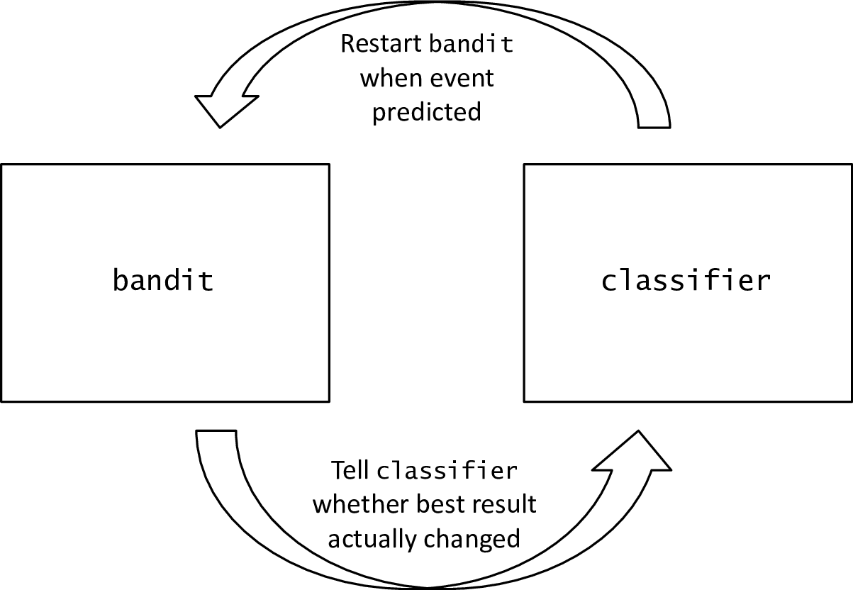
So what prevents us from simply combining an off-the-shelf bandit algorithm with an off-the-shelf classifier? The central challenge is how to define the feedback. Let us outline several hurdles that we need to overcome here. A single false negative prediction will cause bwc to miss an event, which may result in a very high regret (since it may take the bandit algorithm a very long time to adjust). Incorrectly labeled samples may contaminate the classifier, perhaps even permanently. To generate a label for a given sample, one needs to compare the state right before the current round with the state right after, in a conclusive way. Both states are not known to the algorithm a priori, and can only be learned probabilistically via exploration. A particular challenge is to ensure that such exploration is not contaminated by events in the past rounds, as well as by events that happen soon after the current round. Moreover, this exploration is generally too expensive to perform upon negative predictions — indeed, the whole point of bwc is that in the absence of an event the bandit algorithm converges to the best arm and (essentially) keeps playing it — so the classifier receives labels only upon the positive predictions.
4.1 The meta-algorithm
We will present our algorithm in a modular way, as a meta-algorithm which uses the following two components: classifier and bandit. In each round, classifier inputs a context and outputs a “positive” or “negative” prediction of whether an event has happened in this round. Also, it may input labeled samples of the form , where is a context and is a boolean label, which it uses for training. Algorithm bandit is a bandit algorithm that is tuned for the event-free runs.
As described above, we further require bandit to provide feedback to the classifier about whether the best result has actually changed. The standard bandit framework does not immediately provide us with estimates from which such feedback can be obtained. Therefore we require bandit to provide the following additional functionality: after each round of execution, it outputs a pair of subsets of arms;44 4 Following established convention, we call the options available to a bandit algorithm “arms”. In our setting, each arm corresponds to a search result. we call this pair the -th round guess.55 5 Both classifier and bandit make predictions (about events and arms, respectively). For clarity, we will use the term “guess” exclusively to refer to predictions made by bandit, and reserve the term “prediction” for classifier. The meaning of and is that they are algorithm’s estimates for, respectively, the sets of all optimal and (at least) -suboptimal arms. We use to predict whether an event has happened between two runs of bandit. The idea is that any such event causes some arm from of the first run to migrate to of the second run. Accordingly, we generate a negative label if , where and refers to the first and the second run, respectively (see Line 10 of Algorithm 1).
We formalize our assumptions on classifier and bandit as follows:
Definition 1.
classifier is safe for a given concept class if, given only correctly labeled samples, it never outputs a false negative. bandit is called -testable, for some and , if the following holds. Consider an event-free run of bandit, and let be its -th round guess. Then with probability at least , each optimal arm lies in but not in , and any arm that is at least -suboptimal lies in but not in . 66 6 Recall that here is the overall time horizon, as defined in Section 3.
We will discuss efficient implementations of a safe classifier and a -testable bandit in Sections 5 and Section 6, respectively. For bandit, we build on a standard algorithm ucb1 [2]; as it turns out, making it -testable requires a significantly extended analysis.
For correctness, we require bandit to be -testable, where is the minimum shift. The performance of bandit is quantified via its event-free regret, i.e. regret on the event-free runs. Likewise, for correctness we need classifier to be safe, and we quantify its performance via the following property, termed FP-complexity, which refers to the maximum number of false positives.
Definition 2.
Given a concept class , the FP-complexity of classifier is the maximum possible number of false positives it can make in an online prediction game where in each round, an adversary selects a sample, classifier makes a prediction, and then (in some rounds) receives a correct label. Specifically, classifier receives a correct label if and only if the prediction is a false positive. The maximum is taken over all event oracles and all possible sequences of samples.
Now we are ready to present our meta-algorithm, called bwc. It runs in phases of two alternating types: odd phases are called “testing” phases, and even phases are called “adapting” phases. The first round of phase is denoted . In each phase we run a fresh instance of bandit. Each testing phase lasts for rounds, where is a parameter. Each adapting phase ends as soon as classifier predicts “positive”; the round when this happens is round . Phase is called full if it lasts at least rounds. For a full phase , let be the -th round guess in this phase. After each testing phase , we generate a boolean prediction of whether there was an event in the first round thereof. Specifically, letting be the most recent full phase before phase , we set if and only if . If is false, the labeled sample is fed back to the classifier. Note that classifier never receives true-labeled samples. Pseudocode for bwc is given in Algorithm 1.
Disregarding the interleaved testing phases for the moment, bwc restarts bandit whenever classifier predicts “positive”, optimistically assuming that the prediction is correct. By our assumption that events cause some optimal arm to become significantly suboptimal (see Section 3), a correct prediction should result in , where is a phase before the putative event, and is a phase after it. We use this condition in Line 10 of the pseudocode to generate the label. However, to ensure that the estimates and are reliable, we require that phases and are full. And to ensure that the full phases closest to a putative event are not too far from it, we interleave a full testing phase every other phase.
4.2 Provable guarantees
We present provable guarantees for bwc in a modular way, in terms of FP-complexity, event-free regret, and the number of events. This is the main technical result in the paper.
Theorem 1.
Consider an instance of the eventful bandit problem with number of rounds , arms, events and minimum shift ; assume that any two events are at least rounds apart. Consider algorithm bwc with parameter and components classifier and bandit that are, respectively, safe and -testable. Suppose the event-free regret of bandit is bounded from above by a concave function . Then the regret of bwc is
| (1) |
where is the FP-complexity of classifier.
We define a safe classifier whose FP-complexity is bounded in terms of some properties of the underlying concept class (see Section 5). Our instantiation of bandit is -testable for , with concave event-free regret matching that of ucb1 (see Section 6).
The right-hand side of (1) can be parsed as follows. The three summands in (1) correspond to contributions of, respectively, adapting phases, event-free testing phases, and testing phases during which an event has occurred. For the first summand, we show that bwc incurs regret for each adapting phase of length , bound the number of adapting phases by , and then bound the total contribution of all such phases using concavity. For the second summand, we bound the number of clean testing phases by , and note that each such phase contributes at most to regret. For the third summand, each “eventful” testing phase contributes at most to regret, and we show that there can be at most such phases.77 7 In fact, the in the term in (1) can be replaced by the (potentially much smaller) number of testing phases that contain both a false positive in round of the phase and an actual event later in the phase.
Assuming that any two events are at least rounds apart ensures that of any two consecutive phases, one much be event-free. This, in turn, let us invoke the -testability of bandit.
Overview of the proof.
The essential difficulty the analysis of bwc is that an event might happen while the algorithm is testing for another (suspected) event. The corresponding technical difficulty is that the correct operation of the components of bwc — classifier and bandit — is interdependent, so one needs to be careful to avoid a circular argument. In particular, one challenge is to handle events that occur during the first rounds of a phase; these events may potentially “contaminate” the -th round guesses and cause incorrect feedback to classifier.
First, we argue away the probabilistic nature of the problem. We focus on a given testing phase . For each of the two preceding phases , consider the number of events between the first round of phase and the first round of phase . We would like to establish the following separation property: that we can separate (tell apart) the cases of and using the testing condition in Line 10 of the pseudocode. Capitalizing on -testability, we define a technical condition which implies the separation property with very high probability. Regret incurred if the implication “technical condition separation property” 88 8 In the full proof, this implication is called well-detectability. fails to hold is negligible. Thus we can assume that this implication holds always, and argue deterministically from now on.
It is worth noting that we consider two preceding phases because either can be used in in Line 10 of the pseudocode (depending on whether phase is full). A crucial point here is that one of these two phases must be event-free.
Second, we argue that classifier receives only correctly labeled samples. We do it in two steps. Using the well-detectable property, we show that if classifier receives an incorrectly labeled sample after some testing phase , then an event must have occurred during the (adapting) phase . Then using the safety property of classifier, we prove that each adapting phase is event-free.
Third, we bound from above the number of testing and adapting phases, using the maximal number of events and the FP-complexity of the classifier. To this end, we establish that if during a testing phase there are no events, and furthermore there are no events during the two preceding phases, then in the end of bwc generates a correct label . Then the regret bound (1) follows easily from the event-free regret of bandit. ∎
Now let us present the full proof which fills the gaps in the above overview.
Full Proof.
Let be the first round of phase . Recall that phase is called full if it lasts at least rounds. For a full phase , let us say that the phase is event-free if no events happened during interval , and let be the -th round guess in this phase. For two full phases , let us write if and only if . Recall that (as a boolean property) is our algorithm’s estimate of whether there was no event in round .
A testing phase is called well-detectable if for each phase the following property holds: if phases and are full and event-free, then: (i) if there are no events in the interval then , (ii) if in the interval there is exactly one event, then . Since bandit is -testable, each testing phase is well-detectable with probability at least . Thus, with probability at least each testing phase is well-detectable. Thus, regret incurred in the case that a phase fails to be well-detectable is negligible. So in the rest of the proof, we will assume that each testing phase is well-detectable.
We claim that if classifier receives an incorrectly labeled sample after some testing phase , then an event must have occurred during the (adapting) phase . Indeed, by the algorithm specification this sample is , where is the first round of phase . Thus, an event has happened in round , and yet we have , where is the most recent full phase before phase . Since each testing phase is well-detectable, it follows that at least one more event happened between the beginning of phase and the end of phase . Since any two events are at least rounds apart, phase started at some round , and an event has happened in the interval . To prove the claim, it suffices to show that . Now, if phase lasted less than steps, then is a testing phase, and so , contradiction. Thus phase lasted at least steps, and so , claim proved.
We claim that all adapting phases are event-free. For the sake of contradiction, suppose an event occurs during an adapting phase, and let be the first round at which this happens. We know that classifier output a (false) negative in this round, since otherwise a new testing phase would have started at round . Since classifier is safe, at some round before it must have received an incorrectly labeled sample. By the algorithm specification, this must have happened after some testing phase which ended before round . But then (by the previous claim) an event must have occurred during the (adapting) phase , which contradicts the choice of . Claim proved.
From the previous two claims, it follows that classifier receives only correctly labeled samples.
We claim that if there are no events during some testing phases and , then at the end of phase we generate a label . Indeed, suppose not. Then , where is the most recent full phase before phase . Either or ; in either case, implies that there is an event in the interval . Since there are no events during adapting phases, it follows that , contradiction. Claim proved.
We claim that there can be at most testing phases (and hence at most as many adapting phases), including at most event-free testing phases. Indeed, in the first round of each testing phase classifier generates a “positive”, and in the end of the phase we generate a label . We examine each case separately: (i) if then classifier receives feedback, so there can be at most such phases , (ii) if then an event has occurred in phase or , so there can be at most such phases , of which at most phases can be event-free. Claim proved.
5 Safe Classifier
In this section, we show how safe classifiers with low FP-complexity can be constructed for specific concept classes. Recall that a classifier is called safe if (assuming it inputs only correctly labeled samples) it never outputs a false negative, and the definition of FP-complexity, motivated by the specification of the bwc algorithm, essentially assumes that all labeled samples correspond to false positives.
We first describe a generic classifier, called SafeCl, that is safe for any concept class , and bound its FP-complexity using a certain property of . In the event that the concept class is all -dimensional axis-parallel hyper-rectangles with margin , we show that this bound is proportional to . And in the event that the concept class is all -dimensional hyperplanes with margin , we show that this bound is exponential in . Unfortunately, the exponential dependence cannot be improved, as we will see in Section 7.
The classifier SafeCl is defined as follows.
SafeCl classifies a given unlabeled context as negative if and only if there exists no concept such that and for each false-labeled example received so far.
It is easy to see that this classifier is indeed safe. Moreover, we bound its FP-complexity in terms of the following property of the concept class :
Definition 3.
The diameter of , denoted , is equal to the length of the longest sequence such that for each there exists a concept with the following property: , and for all .
Claim 1.
SafeCl is safe, and its FP-complexity is at most .
Proof.
Assume all false-labeled examples input by SafeCl are correctly labeled. Suppose SafeCl outputs a false negative, with concept and unlabeled sample . Then and for each false-labeled example received so far. But by definition of SafeCl such concept does not exist, contradiction. Therefore, SafeCl is safe. Regarding the FP-complexity, consider the prediction game in Definition 2. Any sequence of false positives output by SafeCl satisfies the property in Definition 3, so . ∎
By using SafeCl as our classifier, we introduce into the regret bound of , and this quantity can be large. However, in Section 7 we show that the regret of any algorithm must depend on , unless it depends strongly on the number of rounds .
Below we give examples of common concept classes with efficiently computable safe functions, and prove bounds on their diameter. Recall that for a given universe of examples, a concept is a function , where the null value refers to the examples that are not feasible under a given concept (i.e., if is the true concept, then we will never observe an example such that ).
In what follows, for each define as the set of all for which there is no concept such that and for each . Note that SafeCl outputs a negative prediction on if and only if , where is the set of false-labeled samples received so far. Likewise, in Definition 3 the sequence satisfies for each .
For convenience, define a “-ball” around a set in the -dimensional -norm as
Here is the -norm distance between a point and a set .
5.1 Axis-parallel rectangles with margin
One very simple concept is an axis-parallel hyper-rectangle. This type of concept can be used to test whether any one of several features is outside of its ‘normal’ range. This is a particularly well-suited concept class for predicting events that may affect a search engine query, since these events are typically preceded by a large change in some statistic related to the query, such as its volume or abandonment rate.
Fix the dimension , and let be the -dimensional -norm unit ball around the origin. A -rectangle in is the cross-product of non-empty intervals in . Given and a -rectangle , define a function as follows: equals if ; it equals if , and it equals null otherwise (note that the margin only applies only outside of ). The concept class of -dimensional axis-parallel rectangles with margin is defined as .
We bound the diameter of as follows.
Claim 2.
If , then .
Proof.
Consider a sequence such that for all . Let be the -ball in around the smallest -rectangle containing . By definition of the sequence, at least one of the one-dimensional intervals defining must be larger than the same interval in . Since , . ∎
Clearly, for the concept class , the classifier SafeCl simply maintains the smallest -dimensional rectangle containing the set of all previously false-labeled examples , and classifies a new example as negative if and only if lies within (measured in -norm) of . In other words
SafeCl on : classify as negative , where is the set of all false-labeled examples received so far.
5.2 Hyperplanes with margin
Hyperplanes are perhaps the most widely-used concept in classification problems. Fix the dimension , and let be the -dimensional -norm unit ball around the origin. Given and , define a function as follows: equals if , it equals if , and it equals null otherwise. Here is the unit normal of the hyperplane, and is the shift vector. The concept class of -dimensional hyperplanes with margin is defined as
We bound the diameter of as follows:
Claim 3.
If , then .
Proof.
Consider a sequence such that for all , as in Definition 3. Then for each and such that there exist such that , , and . By Hölder’s inequality, it follows that
| (2) |
Now, place an -ball of radius around each point . By (2), none of these balls can intersect. A radius- ball in dimensions has volume , where is a constant that depends only on . Thus the total volume of the balls is . On the other hand, for each , so each of these balls lies in the radius- ball around the origin, so their total volume is at most . It follows that . ∎
We now show that there is a computationally efficient way to implement the classifier SafeCl for hypothesis class . Specifically, we show that the classifier simply maintains the convex hull of all previously false-labeled examples , classifies a new example as negative if and only if lies within (measured in -norm) of . In other words
SafeCl on : classify as negative , where is the set of all false-labeled examples received so far.
Claim 4.
If and then , where is the convex hull of .
Proof.
Fix . We divide the proof into two parts. First, we show that if is contained in the -ball around , then no hyperplane in can separate from . Next, we show that if is outside the -ball around , then at least one hyperplane in separates from . More precisely, we prove that
- (i)
If then there does not exist such that for all and .
- (ii)
If then there exists such that for all and .
Proof of (i): Suppose for contradiction that there exist , with and , such that for all and .
Choose so that , i.e. is a closest point in to (we know exists because is closed). Since , we have that .
We know that because is a convex combination of the examples in . Therefore, by the intermediate value theorem, there exists and such that and .
Some algebra shows that and . Adding these equations yields
Because , by Hölder’s inequality we have
and
which implies , which is a contradiction.
6 Testable Bandit Algorithms
In this section we will consider the stochastic -armed bandit problem. We are looking for -testable algorithms with low regret. The will need to be sufficiently large, on the order of .
A natural candidate would be algorithm ucb1 from [2] which does very well on event-free regret:
| (5) |
Unfortunately, ucb1 does not immediately provide a way to define the -th round best guess so as to guarantee -testability. One simple fix is to choose an arm at random in each of the first rounds, use these samples to form the best guess, in a straightforward way, and then run ucb1. However, in the first rounds this algorithm incurs regret of , which is very suboptimal compared to from (5).
In this section, we develop an algorithm which has the same regret bound as ucb1, and is -testable. We state this result more generally, in terms of estimating expected payoffs; we believe it may be of independent interest. The -testability is then an easy corollary.
Since our analysis in this section is for the event-free setting, we can drop the subscript from much of our notation. Let denote the (time-invariant) expected payoff of arm . Let , and let be the “suboptimality” of arm . For round , let be the sample average of arm , and let be the number of times arm has been played.
We will use a slightly modified algorithm ucb1 from [2], with a significantly extended analysis. Recall that in each round algorithm ucb1 chooses an arm with the highest index , where is a term that we’ll call the confidence radius whose meaning is that with high probability. For our purposes here it is instructive to re-write the index as for some parameter . Also, to better bound the early failure probability we will re-define the confidence radius as for some parameter . We will denote this parameterized version by .
The original regret analysis of ucb1 in [2] carries over to so as to guarantee event-free regret (5); we omit the details.
Our contribution concerns estimating the ’s. We estimate the maximal expected reward via the sample average of an arm that has been played most often. More precisely, in order to bound the failure probability we consider an arm that has been played most often in the last rounds. For a given round let be one such arm (ties broken arbitrarily), and let will be our estimate of . This estimate (and the provable guarantee thereon) is the main technical contribution of this section.
We obtain an -testable algorithm from , where is the time horizon, by defining the -th round guess as
| (6) |
The pseudocode is in Algorithm 2.
Let us pass to the provable guarantees. We express the “quality” of our estimate as follows:
Theorem 2.
Consider the stochastic -armed bandits problem. Suppose algorithm has been played for steps, and . Then with probability at least for any arm we have
| (7) |
where .
Either we know that is small, or we can approximate it up to a constant factor. Specifically, if then else .
Proof.
Fix round , let and let be the last round this arm has been played before round . Recall that by definition of . Since by pigeonhole principle , it follows that where . It is easy to see that
Then with probability at least for any arm we have
| (8) |
If is the arm with maximal expected reward, then plugging into (8) gives .
Now we are ready for the final calculation. Let be the maximal expected reward. Then
Finally, let us prove that Algorithm 2 is -testable as long as .
Theorem 3.
7 Upper and Lower Bounds
Plugging the classifier from Section 5 and the bandit algorithm from Section 6 into the meta-algorithm from Section 4, we obtain the following numerical guarantee.
Theorem 4.
Consider an instance of the eventful bandit problem with number of rounds , arms, events, minimum shift , minimum suboptimality , and concept class diameter . Assume that any two events are at least rounds apart, where . Consider the bwc algorithm with parameter and components classifier and bandit as presented, respectively, in Section 5 and Section 6. Then the regret of bwc is
While the linear dependence on in this bound may seem large, note that without additional assumptions, regret must be linear in , since each arm must be pulled at least once. In an actual search engine application, the arms can be restricted to, say, the top ten results that match the query.
We now state two lower bounds about eventful bandit problems. Theorem 5 shows that in order to achieve regret that is logarithmic in the number of rounds, a context-aware algorithm is necessary, assuming there is at least one event. Incidentally, this lowerbound can be easily extended to prove that, in our model, no algorithm can achieve logarithmic regret when an event oracle is not contained in the concept class .
Theorem 5.
Consider the eventful bandit problem with number of rounds , two arms, minimum shift and minimum suboptimality , where , for an arbitrary . For any context-ignoring bandit algorithm , there exists a problem instance with a single event such that regret .
Proof.
For simplicity, assume that is an integer. Define problem instances , as follows. In each of these instances, the rounds are partitioned into phases, each of length . There are two arms, call them and . Set for all . For the problem instance , for all . For problem instances , set in all phases , and in all phases . (Thus, in each instance there is a single event that occurs in the first round of phase .)
Now, let be the probability that on problem instance , arm is chosen by algorithm at least once during phase . If for each phase , then on the problem instance each phase contributes at least to regret, so the total regret is at least . Otherwise, for some . Since instances and coincide on the first phases, algorithm behaves the same way on both instances up to the end of phase . Moreover, behaves the same way on both instances throughout phase assuming that it never plays arm during that phase. Therefore with probability its regret on instance due to phase alone is per each round in this phase; so the total regret is at least . ∎
Theorem 6 proves that in Theorem 4, linear dependence on is essentially unavoidable. If we desire a regret bound that has logarithmic dependence on the number of rounds, then a linear dependence on is necessary.
Theorem 6.
Consider the eventful bandit problem with number of rounds and concept class diameter . Let be an eventful bandit algorithm.
- (i)
There exists a problem instance with arms, events, minimum shift , minimum suboptimality , where , for arbitrary , , and , such that .
- (ii)
There exists a problem instance with two arms, a single event, minimum shift and minimum suboptimality such that regret or .
Proof.
For part (i), construct the family of problem instances as follows. In each instance, there are phases of length each. For each phase , one arm, call it , has payoff , and all other arms have payoff . We have one problem instance for each sequence such that for each . Note that there is an event in the first round of each phase; without loss of generality let us assume that this is known to the algorithm. Then in each phase the algorithm (essentially) needs to solve a fresh instance of the stochastic bandit problem on arms with time horizon and payoffs , which implies regret [16, 2]. We omit the easy formal details.
For part (ii), partition the rounds into phases, each of length at least . We define problem instances , in a similar way as in Theorem 5. There are two arms, and . Set for all . For problem instance , set . In problem instance , for , set in all phases , and in all phases . Note that .
In Appendix A, we show how to define the context sequence in a way consistent with all our assumptions, in such a way that the contexts for problem instances and agree in the first phases. The idea is that for both problem instances, the first round of each phase triggers a false positive; this is possible since (essentially) we are allowed false positives.
The rest of the proof involves calculations similar to those in the proof of Theorem 5. First, suppose . Define as in the proof of Theorem 5. If for each phase , then for the problem instance we have . Otherwise, let be such that . By our construction, with probability algorithm behaves identically on instances and through the first phases. Thus, on instance in phase alone it incurs regret per each round of the phase, for a total of .
Next, suppose . Let be the probability that for problem instance , arm is chosen by at least times during phase . If for each phase , then on problem instance . Otherwise, let be such that . In Appendix A, we give a calculation that shows that , which implies that on problem instance . ∎
8 Experiments
To truly demonstrate the benefits of bwc requires real-time manipulation of search results. Since we did not have the means to deploy a system that monitors click/skip activity and correspondingly alters search results with live users, we describe a collection of experiments on synthetically generated data.
We begin with a head-to-head comparison of bwc versus a baseline ucb1 algorithm and show that bwc’s performance improves substantially upon ucb1. Next, we compare the performance of these algorithms as we vary the fraction of intent-shifting queries: as the fraction increases, bwc’s performance improves even further upon prior approaches. Finally, we compare the performance as we vary the number of features. While our theoretical results suggest that regret grows with the number of features in the context space, in our experiments, we surprisingly find that bwc is robust to higher dimensional feature spaces.
Setup: We synthetically generate data as follows. We assume that there are 100 queries where the total number of times these queries are posed is 3M. Each query has five search results for a user to select from. If a query does not experience any events — i.e., it is not “intent-shifting” — then the optimal search result is fixed over time; otherwise the optimal search result may change. Only 10% of the queries are intent-shifting, with at most 10 events per such query. Due to the random nature with which data is generated, regret is reported as an average over 10 runs. The event oracle is an axis-parallel rectangle anchored at the origin, where points inside the box are negative and points outside the box are positive. Thus, if there are two features, say query volume and query abandonment rate, an event occurs if and only if both the volume and abandonment rate exceed certain thresholds.
Bandit with Classifier (bwc): Figure 2(a) shows the average cumulative regret over time of three algorithms. Our baseline comparison is ucb1 which assumes that the best search result is fixed throughout. In addition, we compare to an algorithm we call ora, which uses the event oracle to reset ucb1 whenever an event occurs. We also compared to exp3.s, but its performance was dramatically worse and thus we have not included it in the figure.

| 0 | 1/8 | 1/4 | 3/8 | 1/2 | |
|---|---|---|---|---|---|
| ora | 17.2 | 22.8 | 30.4 | 33.8 | 39.5 |
| bwc | 17.8 | 24.6 | 39.9 | 46.7 | 99.4 |
| ucb1 | 17.2 | 34.1 | 114.9 | 84.2 | 140.0 |
| exp3.s | 78.4 | 123.7 | 180.2 | 197.6 | 243.1 |
| 10 | 20 | 30 | 40 | |
|---|---|---|---|---|
| ora | 21.9 | 23.2 | 21.9 | 22.8 |
| bwc | 23.1 | 24.4 | 22.9 | 23.7 |
| ucb1 | 32.3 | 33.5 | 31.1 | 37.4 |
| exp3.s | 111.6 | 109.4 | 112.5 | 121.3 |
In the early stages of the experiment before any intent-shifting event has happened, ucb1 performs the best. bwc’s safe classifier makes many mistakes in the beginning and consequently pays the price of believing that each query is experiencing an event when in fact it is not. As time progresses, bwc’s classifier makes fewer mistakes, and consequently knows when to reset ucb1 more accurately. ucb1 alone ignores the context entirely and thus incurs substantially larger cumulative regret by the end.
Fraction of Intent-Shifting Queries: In the next experiment, we varied the fraction of intent-shifting queries. Figure 2(b) shows the result of changing the distribution from 0, 1/8, 1/4, 3/8 and 1/2 intent-shifting queries. If there are no intent-shifting queries, then ucb1’s regret is the best. We expect this outcome since bwc’s classifier, because it is safe, initially assumes that all queries are intent-shifting and thus needs time to learn that in fact no queries are intent-shifting. On the other hand, bwc’s regret dominates the other approaches, especially as the fraction of intent-shifting queries grows. exp3.s’s performance is quite poor in this experiment — even when all queries are intent-shifting. The reason is that even when a query is intent-shifting, there are at most 10 intent-shifting events, i.e., each query’s intent is not shifting all the time.
With more intent-shifting queries, the expectation is that regret monotonically increases. In general, this seems to be true in our experiment. There is however a decrease in regret going from 1/4 to 3/8 intent-shifting queries. We believe that this is due to the fact that each query has at most 10 intent-shifting events spread uniformly and it is possible that there were fewer events with potentially smaller shifts in intent in those runs. In other words, the standard deviation of the regret is large. Over the ten 3/8 intent-shifting runs for ora, bwc, ucb1 and exp3.s, the standard deviation was roughly 1K, 10K, 12K and 6K respectively.
Number of Features: Finally, we comment on the performance of our approach as the number of features grows. Our theoretical results suggest that bwc’s performance should deteriorate as the number of features grows. Surprisingly, bwc’s performance is consistently close to the Oracle’s. In Figure 2(b), we show the cumulative regret after 3M impressions as the dimensionality of the context vector grows from 10 to 40 features. bwc’s regret is consistently close to ora as the number of features grows. On the other hand, ucb1’s regret though competitive is worse than bwc, while exp3.s’s performance is across the board poor. Note that both ucb1 and exp3.s’s regret is completely independent of the number of features. The standard deviation of the regret over the 10 runs is substantially lower than the previous experiment. For example, over 10 features, the standard deviation was 355, 1K, 5K, 4K for ora, bwc, ucb1 and exp3.s, respectively.
9 Future Work
The most immediate open question is whether we could train the classifier faster. One idea is to use a more efficient classifier, especially if we can relax the “safety” requirement and somehow recover from false negatives. Another idea is to generate labeled samples not only upon positive predictions but upon negative ones as well, trading off the regret from additional exploration against the benefits of generating extra labeled samples. Finally, it would be desirable to supplement the existing worst-case provable guarantees with stronger ones for settings in which the contexts are sampled from a “benign” distribution.
Theoretically, the main drawback of our approach is that we assume the existence of a “perfect oracle” — a deterministic boolean function on contexts which correctly predicts whether a temporal event has occurred in the current round. It is desirable to extend our results to scenarios in which the contexts allow only approximate or probabilistic prediction. Even though such contexts contain useful signal, exploiting this signal for our purposes appears quite challenging. In particular, it seems to require making the “bandit plus classifier” setup resilient against (infrequent) incorrectly labeled samples and perhaps also against (infrequent) false negatives. It should be noted that the aforementioned resiliency can potentially lead to large improvements in the present oracle-based setting as well, as we might be able to deploy much more efficient classifiers.
Empirically, the main question left for future work is testing the “bandit plus classifier” approach in a realistic setting. The challenge here is two-fold. First, one needs to select which features to use for contexts, and verify experimentally how informative they are in predicting the temporal events. Second, since gaining access to live search traffic is difficult, one would need to simulate it using the search logs, the difficulty being is that the search logs might not have enough data points for alternatives that have not been chosen frequently by the search engine.
Acknowledgements. We thank Rakesh Agrawal, Alan Halverson, Krishnaram Kenthapadi, Robert Kleinberg, Robert Schapire and Yogi Sharma for their helpful comments and suggestions.
References
References
- [1] Deepak Agarwal, Bee-Chung Chen, Pradheep Elango, Nitin Motgi, Seung-Taek Park, Raghu Ramakrishnan, Scott Roy, and Joe Zachariah. Online models for content optimization. In 22nd Advances in Neural Information Processing Systems (NIPS), 2008.
- [2] Peter Auer, Nicolò Cesa-Bianchi, and Paul Fischer. Finite-time analysis of the multiarmed bandit problem. Machine Learning, 47(2-3):235–256, 2002.
- [3] Peter Auer, Nicolò Cesa-Bianchi, Yoav Freund, and Robert E. Schapire. The nonstochastic multiarmed bandit problem. SIAM J. Comput., 32(1):48–77, 2002.
- [4] Sergey Brin and Lawrence Page. The anatomy of a large-scale hypertextual Web search engine. Computer Networks and ISDN Systems, 30(1–7):107–117, 1998.
- [5] Christopher J. C. Burges, Tal Shaked, Erin Renshaw, Ari Lazier, Matt Deeds, Nicole Hamilton, and Gregory N. Hullender. Learning to rank using gradient descent. In 22nd Intl. Conf. on Machine Learning (ICML), 2005.
- [6] Zhe Cao, Tao Qin, Tie-Yan Liu, Ming-Feng Tsai, and Hang Li. Learning to rank: from pairwise approach to listwise approach. In 24th Intl. Conf. on Machine Learning (ICML), 2007.
- [7] Nicolò Cesa-Bianchi and Gábor Lugosi. Prediction, learning, and games. Cambridge University Press, 2006.
- [8] William W. Cohen, Robert E. Schapire, and Yoram Singer. Learning to order things. J. of Artificial Intelligence Research, 10:243–270, 1999.
- [9] Fernando Diaz. Integration of news content into web results. In 2nd Intl. Conf. on Web Search and Data Mining, pages 182–191, 2009.
- [10] D. Fallows. Search engine users. Pew Internet and American Life Project, 2005.
- [11] Yoav Freund, Raj Iyer, Robert E. Schapire, and Yoram Singer. An efficient boosting algorithm for combining preferences. J. of Machine Learning Research, 4:933–969, 2003.
- [12] Elad Hazan and Nimrod Megiddo. Online Learning with Prior Knowledge. In 20th Conference on Learning Theory (COLT), pages 499–513, 2007.
- [13] Thorsten Joachims. Optimizing search engines using clickthrough data. In 8th ACM SIGKDD Intl. Conf. on Knowledge Discovery and Data Mining (KDD), 2002.
- [14] Sham M. Kakade, Shai Shalev-Shwartz, and Ambuj Tewari. Efficient bandit algorithms for online multiclass prediction. In 25th Intl. Conf. on Machine Learning (ICML), 2008.
- [15] Jon M. Kleinberg. Bursty and hierarchical structure in streams. In 8th ACM SIGKDD Intl. Conf. on Knowledge Discovery and Data Mining (KDD), 2002.
- [16] T.L. Lai and Herbert Robbins. Asymptotically efficient adaptive allocation rules. Advances in Applied Mathematics, 6:4–22, 1985.
- [17] John Langford and Tong Zhang. The epoch-greedy algorithm for multi-armed bandits with side information. In 21st Advances in Neural Information Processing Systems (NIPS), 2007.
- [18] Sandeep Pandey, Deepak Agarwal, Deepayan Chakrabarti, and Vanja Josifovski. Bandits for Taxonomies: A Model-based Approach. In SIAM Intl. Conf. on Data Mining (SDM), 2007.
- [19] Sandeep Pandey, Deepayan Chakrabarti, and Deepak Agarwal. Multi-armed Bandit Problems with Dependent Arms. In 24th Intl. Conf. on Machine Learning (ICML), 2007.
- [20] Filip Radlinski, Robert Kleinberg, and Thorsten Joachims. Learning diverse rankings with multi-armed bandits. In 25th Intl. Conf. on Machine Learning (ICML), 2008.
- [21] R. Tyrrell Rockafellar. Convex Analysis. Princeton University Press, Princeton, NJ, 1970.
- [22] Chih-Chun Wang, Sanjeev R. Kulkarni, and H. Vincent Poor. Bandit problems with side observations. IEEE Trans. on Automatic Control, 50(3):338355, 2005.
- [23] Jia Yuan Yu and Shie Mannor. Piecewise-stationary bandit problems with side observations. In 26th Intl. Conf. on Machine Learning (ICML), 2009.
Appendix A Details for the proof of Theorem 6(ii)
Claim 5.
We can define context sequences and with the following properties: (1) each sequence , when paired with a problem instance , defines an eventful bandit problem consistent with all our assumptions, and (2) the sequences and agree through the first phases.
Proof.
Let be a sequence of contexts such that for all . We know this sequence exists by the definition of . Also assume there exists an “always negative” context such that for all (this assumption is not necessary, but is convenient). Let be the first round of phase .
Define as follows: let for each phase , and let for all other rounds.
For , define as follows: let for each phase , and let for all other rounds.∎
Claim 6.
Proof.
Throughout this proof, we fix phase . Define a realization to be a particular sequence of outcomes of all random samples from click distributions, as well as all random choices (if any), during an execution of algorithm through the end of phase . For example, if is a realization, then might correspond to the click observed in the first round, might correspond to random choices made by the algorithm, might correspond to the click observed in the second round, and so on. By the chain rule, for any :
For any realization , let be the product of terms in the above product that correspond to outcomes other than observed clicks in phase . Let be the set of realizations in which arm is selected by less than times in phase . Let be the number of times in realization that arm is selected in phase and payoff is observed as a result. Then