A scalar field condensation instability of rotating anti-de Sitter black holes
Abstract
Near-extreme Reissner-Nordström-anti-de Sitter black holes are unstable against the condensation of an uncharged scalar field with mass close to the Breitenlöhner-Freedman bound. It is shown that a similar instability afflicts near-extreme large rotating AdS black holes, and near-extreme hyperbolic Schwarzschild-AdS black holes. The resulting nonlinear hairy black hole solutions are determined numerically. Some stability results for (possibly charged) scalar fields in black hole backgrounds are proved. For most of the extreme black holes we consider, these demonstrate stability if the “effective mass” respects the near-horizon BF bound. Small spherical Reissner-Nordström-AdS black holes are an interesting exception to this result.
1 Introduction
Charged black holes in anti-de Sitter space have played an important role in recent discussions of superconductivity based on the gauge/gravity correspondence. The simplest model of this phenomenon consists of gravity coupled to a Maxwell field and a charged scalar field [1]. The non-superconducting phase is dual to the Reissner-Nordström-AdS black hole solution, which is stable at sufficiently high temperature. However, at temperature below a certain critical value, this solution is unstable against condensation of the scalar field. At these low temperatures there exists a new charged black hole solution, with a non-trivial scalar field present. This describes the superconducting phase.
Surprisingly, the condensation can occur even when the scalar field is uncharged [2]. A nice way of understanding this is to consider the special case of an extreme (planar) Reissner-Nordström-AdS black hole. This has near-horizon geometry. The Breitenlöhner-Freedman bound [3, 4] required for stability of the lies above that required for stability of the asymptotic . This suggests that an uncharged scalar field which satisfies the BF bound but violates the BF bound will be unstable in the extreme RN-AdS background.11 1 Ref. [2] attributed this argument to M. Roberts. This is confirmed by solving numerically the scalar equation of motion in the black hole background [2, 5].
The motivation for the present paper is the observation that extreme, rotating, AdS black holes also have near-horizon geometries containing an factor. Hence one might expect that a scalar condensation instability will afflict these black holes too.22 2 It was shown in Ref. [6] that the charged scalar condensation instability of static charged AdS black holes extends also to rotating charged AdS black holes. In our work, neither the scalar field nor the black hole is charged. We shall confirm that this is indeed the case for black holes sufficiently close to extremality.
We shall consider the (topologically spherical) rotating black hole solutions discovered by Hawking, Hunter and Taylor (HHT) [7] (sometimes called Myers-Perry-AdS). In general these have two angular momenta but we shall set these equal since the solution then depends non-trivially only on a single radial coordinate . These solutions can be parameterized by the horizon radius and the angular velocity . At extremality, the BF bound is above the bound if (where is the radius), i.e., for “large” black holes. In this case, we might expect scalar condensation to occur if the scalar mass lies between the two BF bounds.
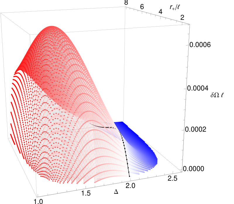
We have determined numerically the values of , and the scalar mass for which there exists a time-independent solution of the scalar field equation of motion which preserves the symmetries of the background. Such a solution is expected to arise at the threshold of the instability. Figure 1 summarizes the result of this calculation. The condensate appears only when the black hole is very close to extremality: typical temperatures are .
The analogy with the charged case suggests that the endpoint of the instability should be a 2-parameter rotating black hole solution with scalar hair. This new solution should have the same symmetries as the HHT solution, so it will have equal angular momenta. We have determined certain 1-parameter subfamilies of this solution numerically (taking to saturate the BF bound). We find that the hairy black holes have higher entropy than the HHT black holes with the same mass and angular momenta. Hence it is consistent with the second law for the HHT black hole to evolve to our new hairy solutions. Our numerical results suggest that the entropy of the hairy black holes will vanish as the temperature approaches zero, just as in the charged case [8, 9, 10].
We have extended the linear analysis to the four-dimensional Kerr-AdS solution. Again, we found that a scalar condensation instability occurs in a region close to extremality. Since this solution depends non-trivially on two coordinates ( and ), we did not attempt to construct numerically the corresponding hairy black holes. Note that it has been proved that a scalar field that respects the BF bound is stable in a sufficiently slowly-rotating Kerr-AdS background [11]. Our results show that this conclusion does not extend to rapidly rotating Kerr-AdS black holes.
Our results have implications for (conjectured) no hair theorems. Consider AdS gravity coupled to an uncharged scalar field. Ref. [12] conjectured that static spherically symmetric hairy black hole solutions do not exist if the theory admits a positive energy theorem with boundary conditions that preserve the symmetries of AdS. Our results demonstrate that this conjecture cannot be extended to non-static black holes.
For Reissner-Nordström-AdS, the instability against condensation of an uncharged scalar can co-exist with an instability against condensation of a charged scalar. In the rotating case, the analogue of the scalar field charge is the angular momentum quantum number of the scalar field, which we have set to zero. However, for , black holes with exhibit a superradiant instability [13]. This is the analogue of charged scalar condensation. Now, since extreme black holes always have , and scalar condensation with occurs only very close to extremality, it follows that the scalar condensation instability studied in this paper always coexists with the superradiant instability. Moreover, the new hairy black holes that we find have . Therefore they are likely to suffer from a superradiant instability themselves. The endpoint of this kind of instability is unknown.
Two other topics are studied in this paper. First, we note that a nice toy model for the study of uncharged scalar field condensation is the Schwarzschild-AdS black hole with hyperbolic spatial slices. This solution has a regular extreme limit (in contrast to the spherical or planar Schwarzschild-AdS black hole) with an in the near-horizon geometry. We determine the range of values for and for which scalar condensation occurs. The resulting 1-parameter nonlinear hairy black hole solution is determined numerically (for particular ).33 3 We note that previous work has found a similar solution analytically by including a suitably chosen scalar potential [14]. We emphasize that we are working with a free (and minimally coupled) scalar. Another difference is that we use AdS invariant boundary conditions at infinity, which does not appear to be the case for the solution of Ref. [14].
Second, we shall present some stability results concerning scalar condensation. The idea is to construct an “energy” functional for the scalar field (which might not coincide with the usual energy) which is manifestly non-increasing in time. If one can show that this energy is positive definite then an initially small fluctuation in the field must remain small, i.e. condensation does not occur. Demonstrating positivity is non-trivial because we are mainly interested in the situation in which . Fortunately, this problem has been addressed in Ref. [11] for spherical Schwarzschild-AdS black holes so we can generalize this method. For the extreme black holes considered in this paper, we show that the energy is positive definite if, and only if, the BF bound is satisfied. Our numerical results demonstrate that an instability appears as soon as the bound is violated. For non-extreme black holes, our method gives a lower bound on that guarantees stability although this bound is not sharp.
The method can also be applied to a charged scalar field in a Reissner-Nordström-AdS background. For planar, hyperbolic or sufficiently large spherical black holes, our energy functional is positive definite at extremality if, and only if, the near-horizon “effective mass” satisfies the BF bound. For the planar case, Ref. [5] found numerically that an instability occurs precisely when this bound is violated. Small spherical extreme RN-AdS black holes are an interesting exception: for these our stability bound is more restrictive than the near-horizon BF bound and indeed Ref. [9] found an instability even when the near-horizon BF bound is respected.
This paper is organized as follows. We state the problem in Section 2. We then discuss in Section 3 the hyperbolic Schwarzschild-AdS black hole as a toy model to illustrate the scalar condensation phenomenon. Next we discuss rotating AdS black holes: cohomogeneity-1 solutions in Section 4 and also the four-dimensional Kerr-AdS in Section 5. In Section 6 we present our stability results for scalar condensation.
2 Scalar condensation
Consider a scalar field with mass in an asymptotically background. It satisfies the Klein-Gordon equation,
| (1) |
and always decays at infinity as [3, 4]
| (2) |
and is the AdS radius. Stability of the AdS background requires reality of , i.e. that the mass of the scalar field must obey the Breitenlöhner-Freedman (BF) bound [3, 4]
| (3) |
For scalars with mass above this BF bound and below the unitarity bound, i.e.
| (4) |
there is a choice of boundary conditions: one can impose either that decays as or as , since both give normalizable solutions. In the AdS/CFT correspondence, this choice dictates whether the operator dual to has dimension or [15]. For masses above the unitarity bound only the mode with the faster fall-off, , is normalizable.
Now consider an extreme, asymptotically black hole whose near-horizon geometry contains an factor with radius . The BF bound associated to this is
| (5) |
Hence if
| (6) |
then the asymptotic will be stable but the near-horizon geometry is unstable. This suggests that the full black hole solution will be unstable against scalar condensation [2]. This has been confirmed by numerical calculation in certain cases [5].
3 Toy model: hyperbolic Schwarzschild-AdS
3.1 Introduction
The simplest black hole that exhibits the scalar condensation phenomenon is the Schwarzschild-AdS solution with hyperbolic spatial sections. Consider the general Schwarzschild-AdS solution in dimensions:
| (7) |
where is the metric on a unit sphere (), hyperboloid (), or flat space () that satisfies . The function is given by
| (8) |
where the horizon is at .
For , the horizon is always non-degenerate. However, for a black hole solution exists for
| (9) |
and has Hawking temperature
| (10) |
An extreme (zero temperature) regular solution is present when the bound in (9) is saturated. This extreme solution has near-horizon geometry , where the has radius . Hence scalar condensation seems likely when the scalar mass lies between the and BF bounds:
| (11) |
If lies strictly above the BF bound then the stability argument that we shall present in Section 6 below demonstrates that the scalar field is stable for sufficiently large . However, if also lies below the near-horizon BF bound for the extreme black hole then we expect the scalar field to become unstable as extremality is approached, i.e. as decreases. At the value of corresponding to the threshold of instability, we expect there to exist a time-independent solution of the scalar equation of motion44 4 See Refs. [16, 17] for previous studies of scalar fields in the hyperbolic Schwarzschild-AdS spacetime.
| (12) |
We shall confirm the existence of this solution numerically.
We note that the entropy and energy of the black hole are given by
| (13) |
where is the volume of the hyperboloid (which we shall assume to be compactified).
The solution with is special: this solution is locally isometric to and has zero energy. Solutions with have negative energy with the extreme solution having the lowest energy.
3.2 Numerical results: linear
For definiteness, we set . For scalar mass below the unitarity bound we shall consider both choices of boundary condition. For this reason, it is more convenient to work with the dimension of the operator dual to the scalar field than with . For given we wish to determine the value of for which there exists a solution that is regular at the horizon and decays as at infinity. We do this using a standard shooting method where we construct power series solutions near the horizon and at infinity up to seventh order and then evolve the solution away from these points numerically. Fixing the amplitude of the solution at spatial infinity, we impose matching conditions, namely the continuity of and , at some fixed value of . We find that matching is possible only for a particular value of .
The results are presented in Figure 2. The black hole is extreme for . The near-horizon BF bound (which lies above the unitarity bound) corresponds to . This is indeed the limiting value of the curve at the extremal blue point.55 5 This blue point is a limit of the curve, it does not belong to the curve. This is because, at extremality, there is no regular time-independent solution associated to the threshold of instability. The scalar field diverges at the horizon if one takes a limit of the time-independent solution associated to the threshold of instability of non-extreme solutions. Hence our results agree with the expectation that scalar condensation occurs for the extreme solution if, and only if, the near-horizon BF bound is violated. For , we find no solution, so there is no scalar condensation instability for any . However, as decreases through , first the extreme black hole becomes unstable and then the critical temperature below which the black hole is unstable increases monotonically.
Saturation of the BF bound corresponds to . Our numerical results suggest that the threshold of instability for occurs at . One can confirm analytically that the black hole with admits the regular solution if . As mentioned above, the solution is special: it is locally isometric to . Our results imply that this solution is unstable against scalar perturbations with . But is stable! The point is that our solution is isometric only to part of . If one analytically extended an unstable mode of our solution to global then either it would not be regular everywhere or it would not satisfy the appropriate boundary conditions at infinity. Hence it would not correspond to an instability of so there is no contradiction.
3.3 Numerical results: nonlinear
In this subsection, we construct the family of hairy black holes that branches-off from the original Schwarzchild-AdS black hole family in a phase diagram of static and neutral solutions with an hyperbolic horizon topology.
We employ two different methods that agree in the regime where they have to. First, we follow an analytical perturbative approach. Starting with an appropriate ansatz for the hairy black hole solution, we expand out the gravitational and scalar fields in a power series of a small parameter . This is a measure of the value of the scalar field at infinity and indicates the deviation of the hairy solution from the unstable Schwarzchild-AdS black hole. We do this perturbative expansion up to order. To obtain the exact result, we then do a full non-linear numerical construction of the hairy black hole solution. We present our results in subsection 3.3.3 where we describe our findings in a phase diagram of static and neutral solutions with an hyperbolic horizon topology.
3.3.1 Hairy black hole ansatz. Equations of motion
We want to look for hairy black hole solutions with an hyperbolic horizon topology. As in the linear analysis, we consider . Therefore we take the following ansatz for the gravitational and scalar fields,
| (14) |
When , and is given by (8) with , the system describes the hyperbolic Schwarzchild-AdS black hole. This ansatz solves the equations of motion derived from the Einstein-scalar action,
| (15) |
if the following equations are satisfied,
| (16a) | ||||
| (16b) | ||||
| (16c) | ||||
Given , can be easily found through the integration of (16c). So the problem at hand reduces to determining and .
The boundary conditions to be imposed are as follows. We use the scaling symmetry of the equations of motion, and (with the other variables/fields unchanged) to set at the asymptotic boundary without loss of generality. At the horizon we demand that is regular. The function must vanish at the horizon, and we take this condition as our definition for the location of the black hole horizon. We require the hairy black hole to be asymptotically AdS and thus must behave as at large distances. On the other hand, the scalar field has to be regular at the horizon. Its asymptotic boundary condition is determined by the requirement of normalisability at infinity. In our linear analysis we found that a hairy black hole should exist only for scalar masses above the BF bound and below the NH BF bound. Therefore we restrict our attention to this range of masses. For concreteness we consider the simplest case (and thus ) for which an analytical perturbative construction is possible and where the numerics simplify considerably. Summarizing, the boundary conditions for the non-linear problem are:
| (17) |
For an explicit construction of the hairy black hole we should still select a particular hyperbolic Schwarzchild-AdS black hole to which the hairy black hole should reduce in the limit where the scalar field vanishes, i.e. a particular value of in (8) (with ). We are taking so will find the hairy black hole that bifurcates from the hyperbolic Schwarzchild-AdS black hole with . This choice is not arbitrary. Indeed in this case we can solve analytically the equation (12) that gives the perturbative leading order scalar field. This can then be used to generate the next-to-leading order expansion terms. Ultimately, we will then use this perturbative result as the seed solution in the relaxation method employed to construct numerically the exact hairy black hole. To sum up, our selection of parameters is
| (18) |
3.3.2 Perturbative and numerical construction of solution
To construct perturbatively the hairy black hole, we expand all the unknown functions of the system, namely , and in a power series of ,
| (19) |
where is a measure of the scalar field at infinity. Using a standard perturbation theory strategy, we plug these expansions in the equations of motion (16) to solve for the coefficients , and . In short, the procedure at each order is the following. Equation (16b) is used to solve for , up to an integration constant. The boundary condition must be satisfied at each order and is used to find , which defines the horizon location where some of the boundary conditions will be imposed. We can now use (16a) to solve for , again up to integration constants. The boundary conditions (17) are now imposed to constraint the integration constants generated in the process. Finally, also has an expansion in that can at this point be easily found by direct integration of (16c).
At leading order, , the scalar field is given by while and . That is, we are in the linear regime discussed in the previous section, where the back-reaction in the gravitational field is neglected and solves (12) (note that the analytical solution is possible only because we perturb the black hole with ). We will find that for our purposes it will be enough to do the expansion up to order . The explicit expression for the expansion functions up to order would be far too cumbersome and not illuminating at all. For illustration purposes we just give the result up to the order,
| (20) |
The result of the perturbative analysis up to order will be presented in the phase diagrams of subsection 3.3.3.
The most efficient way to get the full information on hairy black holes in the phase diagram of solutions is to resort to a full non-linear numerical approach that solves non-perturbatively the equations of motion (16). Our numerical strategy to find the exact hairy black hole is to use a standard relaxation method [18], with a spectral discretization of the integration grid [19]. Again, we have to solve the system of coupled ODEs (16a) and (16b) subject to the boundary conditions (17), and for the selection of parameters (18).
The implementation of the boundary conditions using the spectral discretization is simpler if we implement the following redefinition of the fields,
| (21) |
in which case the boundary conditions (17) reduce to
| (22) |
The factor in the relation for in (21) guarantees that the field redefinition does not introduce a new critical (singular) point in the differential equations to be solved (i.e. besides the boundary critical points). Our numerical results for the hairy black hole will be presented in the next subsection.
3.3.3 Phase diagram
In this subsection we present the properties of the hairy black holes that we constructed using the perturbative and numerical approaches described in the previous subsection. We present the scalar condensate, the temperature and the entropy of the hairy black hole as a function of its energy.
To compute the energy of the hairy black hole in AdS we use the Astekhar-Das formalism [20]. The temperature, entropy and energy of the hairy black hole are given by
| (23) |
where the energy is measured with respect to the AdS background. is the volume of the (compactified) hyperboloid of unit radius, is the coefficient in the large expansion of and is the coefficient in the large expansion of . We will compare these thermodynamic quantities with those for the family of hyperbolic Schwarzchild-AdS black holes. Henceforth we shall set , equivalently and can be regarded as energy and entropy per unit hyperboloid volume.
In Fig. 3, we plot the value of the condensate at infinity, as defined in (17), as a function of the dimensionless energy of the hairy black hole (equivalently: we are plotting the vev of the operator dual to our scalar field). The condensate vanishes in the limit where the hairy black hole reduces to the Schwarzchild-AdS black hole with , which has zero energy. The condensate then increases as the energy grows negative. The red curve describes the results obtained using the analytical perturbative construction of section 3.3.2, while the blue curve describes the exact numerical results using the relaxation method of section 3.3.2. The matching of these two curves is very good for absolute values of the energy that are not too large, as it should be.
In Fig. 4, we plot the dimensionless temperature, (left), and dimensionless entropy, (right), of the hairy black hole as a function of its dimensionless energy . Again, the red (blue) curve describes the results obtained using the perturbative (numerical) construction of section 3.3.2. Once more these two curves coincide for absolute values of the energy that are small. The perturbative construction up to the order in the expansion starts deviating from the numerical curve only for energies smaller than (say). In these plots, we also display in a dashed black line the temperature and entropy of the hyperbolic Schwarzchild-AdS black hole family. We display this family only for which corresponds to a range of (non-positive) energies where it co-exists with the hairy black hole. At , we have the Schwarzchild-AdS black hole with zero energy, from which the hairy black hole solution bifurcates. As we decrease the energy of the Schwarzchild-AdS family, the temperature and entropy starts decreasing until the extreme black hole with , and non-vanishing entropy is reached.
Our results above show that hyperbolic Schwarzschild-AdS black holes with () are unstable against condensation of a free scalar field dual to a CFT operator. The threshold mode of this instability is identified as a black point in Fig. 2. In the phase diagrams of Fig. 4, this zero-mode signals a bifurcation point at in the Schwarzchild-AdS family of solutions into a new branch of hairy black holes. For fixed energy where the two families co-exist, the hairy black holes always have higher temperature and entropy than the Schwarzschild-AdS black holes. So we have a second order phase transition. As the energy decreases, the temperature and entropy of the hairy black hole decrease. This family of solutions ends in a zero temperature state where both the temperature and the entropy of the hairy solution vanish. This configuration is represented by a green point in the phase diagrams. Using the information from both phase diagrams we find this state to have an energy of with an estimated error based on both plots of .
It is worth commenting on the nature of the zero temperature limit of these hairy black holes. The fact that the entropy appears to vanish in this limit is good evidence that the limiting geometry is not an extreme black hole. Further evidence for this comes from the fact that if a hairy extreme black hole did exist then the scalar field would be constant in its near-horizon geometry. But then the scalar equation of motion would imply that the scalar field must be zero in the near-horizon geometry (this argument is due to Ref. [21]). This would imply that the scalar must vanish at the horizon of the full extreme black hole. However, our numerical results indicate that the value of the scalar field at the horizon increases as the temperature decreases. Hence the zero temperature limit cannot be an extreme black hole. A similar conclusion has been obtained in the case of charged scalar condensation in Reissner-Nordström-AdS [8].
4 Rotating black holes with equal angular momenta
4.1 Introduction
The HHT black hole [7] with equal angular momenta is the case of a family of “Myers-Perry-AdS” black holes [22, 23] with cohomogeneity-1. These solutions exist in odd dimensions , and the metric can be written as:66 6 The radial coordinate used here can be related to the standard Boyer-Lindquist radial coordinate of [22, 23] through . The functions used here are related with the functions used in [13] through , and .
| (24) |
where
and is the Fubini-Study metric on with Ricci tensor , and is related to the Kähler form by . Surfaces of constant and have the geometry of a homogeneously squashed , written as an fibred over . The fibre is parameterized by the coordinate , which has period .
The spacetime metric satisfies . Asymptotically, the solution approaches anti-de Sitter (AdS) space with radius of curvature . The event horizon is located at (the largest real root of ) and it is a Killing horizon of , where the angular velocity of the horizon is given by:
| (25) |
The solution saturating the bound in the angular velocity corresponds to an extreme black hole with a regular, but degenerate, horizon. Note that this upper bound in is always greater than and tends to the unit value in the limit of large .
We shall find it convenient to parameterize the solution in terms of instead of through the relations,
| (26) |
The temperature of the black hole,
| (27) |
vanishes for the extreme configuration. The mass and angular momentum , defined with respect to , are [24] (taking )
| (28) |
where is the area of a unit ()-sphere.
Once again, we shall look for a time-independent solution of the scalar wave equation that we expect to signal the onset of instability. We shall assume the scalar field to be axisymmetric (with respect to ), i.e., it preserves the symmetry associated to the rotation of the background. However, we shall allow for the possibility that the scalar breaks the symmetry of . We take the field to have the separable form . Here, is a scalar harmonic of , with Laplacian eigenvalue given by , . The scalar wave equation reduces to
| (29) |
In the extreme case, the near-horizon geometry is homogeneous and takes the form of a fibration over . From the above equation we can read off an “effective mass” for the scalar field near the horizon: . The near-horizon BF bound (determined by the radius of the ) is
| (30) |
We are interested in whether it is possible to violate this bound whilst respecting the BF bound (3). A short calculation reveals that this is possible if, and only if,
| (31) |
So we expect an instability only for black holes larger than the AdS length . Furthermore, modes with should be the most unstable since they have the lowest . Written out explicitly, we expect an instability of the extreme black hole if the scalar mass lies in the range
| (32) |
Another interesting 5d black hole solution is the supersymmetric black hole of Ref. [25]. In this case, we find that the near-horizon BF bound coincides with the bound so there is no reason to expect a scalar condensation instability. We shall not consider this solution further.
4.2 Numerical results: linear
4.2.1 Numerical methods
We will solve Eq. (29) numerically in search of the onset of the scalar condensation. This is a boundary value problem. The appropriate boundary conditions can be found through a standard Fröbenius analysis. At the horizon, regularity of the solution requires that the scalar field must be finite, while at the asymptotic region the scalar field decays as
Stability of the AdS background requires that the scalar field must obey the Breitenlöhner-Freedman bound (3). Both fall-offs in (4.2.1) can be normalizable so we can impose one of the two boundary conditions: or .
At this point we make the important observation that the radial equation (29) can be written as a generalized eigenvalue problem in . That is, we can cast (29) in the form
| (34) |
where and are both second order differential operators that do not depend on . For fixed and , our strategy for finding a zero-mode for the scalar condensation will be to determine the eigenvalue for which there exists a solution of (34) that is regular at and satisfies the appropriate boundary condition (either or ) at . This strategy is motivated by the availability of numerical techniques for solving eigenvalue equations of the form (34). More concretely, we solve this equation using a spectral numerical method. This method already proved to be suitable to study perturbations in black hole backgrounds [26, 27, 28]. The application of the method is simpler for Dirichlet and/or Neumann boundary conditions. Therefore we introduce the following perturbation functions,
| (35) |
and we impose the Dirichlet boundary condition at the horizon and the Neumann boundary condition at infinity,
| (36) |
that guarantee that the boundary conditions discussed above for are satisfied. In these equations the choice of applies if we want to study the case where in (4.2.1), while choosing the function allows us to address the case . For the numerical implementation, it is convenient to use the variable
| (37) |
instead of the radial coordinate , since is dimensionless and bounded, . We will also use a scaling symmetry of the radial equation to normalize all our quantities in units of the cosmological length. Then equation (29) or (34) depends only on four dimensionless parameters, namely, , , and (or, equivalently, ). The strategy is now to fix and run the spectral numerical code for several values of and and find the eigenvalues of (34). These will be presented in Section 4.2.2.
As a double check, we will also use a shooting method to reproduce some of our results. A further motivation to use this second numerical method is that it allows us to find the important tail on the lower region of Figure 5 with better accuracy.
In the shooting method, the numerical strategy is the following. Again we want to fix , and and find at the onset of the instability. Equation (29) has two critical points: at the horizon and at infinity. We first focus our attention at the horizon. Using a Taylor series expansion, we construct the solution in the near-horizon region up to the eighth order in the radial distance to the horizon. Fixing , this solution depends on but also on an arbitrary amplitude . We then integrate numerically the radial second order ODE, using a standard fourth order Runge-Kutta method, up to a large radial distance. We repeat the procedure, this time at the asymptotic critical point where we start by obtaining the asymptotic solution up to eighth order. Again this solution is a function of and of an arbitrary amplitude that we set equal to . We integrate this solution down to very small values of the radial distance. In the overlapping region of the two solutions we then do their matching. The requirement that both the scalar field and its radial derivative must be continuous fixes the values of the two unknowns, namely the desired and the amplitude . The whole process is now repeated for a grid of values at fixed to generate the results in Section 4.2.2.
A subtlety intrinsic to the system at hand and not so standard in shooting applications is that the onset of our instability occurs close to the extreme solution. The Taylor expansion of the near-horizon solution is in terms of powers of , where is the compact radial coordinate defined in (37). Therefore, since the instability we search for sets in very close to extremality, typically the near-horizon expansion breaks down. To avoid this we work with a new compact radial coordinate defined as
| (38) |
4.2.2 Results
We expect an instability if we satisfy (32). The simplest equal spin MP system that captures all the features of the scalar condensation instability is the case with . Therefore we will present most of our results for this case, and in the end we will discuss the and/or cases.
In , and one has , and , with . Therefore both normalizable modes with fall-off should be unstable for masses obeying the condition (32) (for this is not true for large enough ). This is precisely what we find numerically, following the strategy outlined in the previous section, as shown in Figure 1. In this figure, we plot the dimensionless angular velocity (measured wrt the extreme angular velocity ) at which the HHT black hole has the zero-mode for the scalar condensation instability, as a function of the dimensionless horizon radius and of the conformal dimension(s) defined in (2). The red curves describe the modes with faster fall-off , the blue curves describe the modes with fall-off , and the single black curve is precisely at the BF bound where .
The expectation is that for fixed , all black holes that are in the parameter space below this surface are unstable and decay into hairy black holes with a scalar condensate surrounding the horizon. That is, the HHT black hole is stable for sufficiently high temperatures, but, for given and , there is a critical temperature where it becomes marginally unstable against scalar condensation, and for lower values of the temperature the black hole is unstable. Note that the surface extends to arbitrarily large .
For clarity, we also plot the curve as a function of for a fixed value of the scalar mass in Figure 5; for concreteness we picked the black curve in Figure 1 where . Note that the “tail” on this curve extends all the way down to an extremal solution with (something that is not apparent from Figure 1). But, for , this is precisely the threshold of instability predicted by the near-horizon BF bound. In more detail, for the near-horizon BF bound is violated if, and only if, . Hence we have numerical evidence that this bound is sharp: an instability appears as soon as it is violated.77 7 Just as for the hyperbolic black hole, the extreme solution does not admit a regular time-independent solution associated to the threshold of instability. If one takes the limit of the time-independent solution associated to non-extreme solutions then the value of the scalar field at the horizon diverges at extremality.
The instability against the scalar condensation is not the only instability present. Indeed, it competes with the well-known superradiant instability that afflicts rotating AdS black holes whenever [13]88 8 The superradiant instability is associated to perturbations that break the symmetry generated by . This instability is not confined to the scalar field, e.g., it is also present for gravitational perturbations.. Since there is competition between the two instabilities it is relevant to ask whether the scalar condensation instability occurs when . We find a negative answer. Recall that extreme black holes always have . Figure 1 shows that condensation occurs only when is very close to , and we have checked that this implies that . So the scalar condensation instability studied here always co-exists with the superradiant instability.

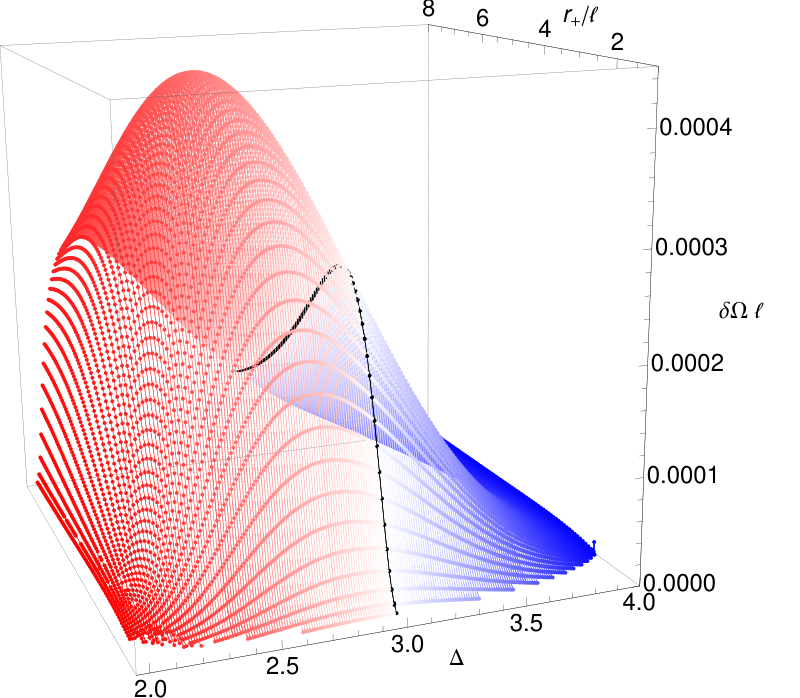
We can now discuss what happens when we turn on the dependence defined in terms of the non-negative integer . We find zero-modes of the instability for , at least up to . As the simplest example, in the left plot of Figure 6, we show the properties of the instability for and . The stationary axisymmetric mode is indeed still present but the instability sets in for lower temperatures. Indeed the maximum difference between the extreme value of the HHT angular velocity and the angular velocity where the instability switches on is smaller in the left plot of Figure 6 than in the case shown in Figure 1. For it is still true that the instability persists all the way up to the NH BF bound. To check this we take again as a reference point the curve . In this case, according to the condition (32), the zero-mode of the instability should kick in at extremality at the critical value of given by (31). This value increases as grows. For , it is . Our numerical results indeed confirm that the zero-mode of the instability is present for values of at and above this value. This can be inferred by the range of in the left panel of Figure 6, although a precise check requires analyzing the tail that develops close to extremality like we did for in Figure 5.
Finally, let us discuss what happens as the dimension parameter grows. We have explicitly checked the cases and the instability is still present. The numerical results for and are presented in the right panel of Figure 6. As grows, the instability sets in for black holes that are closer to extremality, i.e. that have lower values of . For , the instability persists all the way down to when , in agreement with the conditions (31) and (32) for the existence of the instability.
4.3 Numerical results: nonlinear
In the previous subsection, we found the properties of the onset of the scalar condensation instability in the codimension-1 Myers-Perry-AdS black hole. In this subsection, we include the backreaction in the gravitational field and construct the hairy codimension-1 rotating black holes that are associated with this instability.
4.3.1 Hairy black hole ansatz. Equations of motion
We want to look for hairy black hole solutions that reduce to the codimension-1 Myers-Perry black hole (24) when the scalar condensate vanishes, and that preserve the isometries of the latter solution. Therefore we take the following ansatz for the gravitational and scalar fields,
| (39) |
where, as before, is the Fubini-Study metric on , and is the Kähler potential of . When the condensate vanishes, , and , (39) describes the MP solution (24) after performing the radial coordinate transformation . This ansatz solves the equations of motion derived from the Einstein-scalar action (15) when the following equations are satisfied (taking , i.e., henceforth)
| (40a) | ||||
| (40b) | ||||
| (40c) | ||||
where the system of three ODEs described in (40a) is cumbersome and thus we leave its explicit expressions for equation (91) of Appendix B.
The construction of the hairy black hole amounts to determining , and that solve the system (40), i.e. (91), and (40c). Once these are known, is straightforwardly obtained from (40b). The constant in (40c) is linearly proportional to the angular momentum of the solution, as we shall confirm later.
The boundary conditions are the following. The function must vanish at the horizon, and we take this condition as our definition for the location of the black hole horizon. We require the hairy black hole to be asymptotically AdS and thus must approach asymptotically. For the same reason, must go to the unit value at infinity, while vanishes there. At the horizon we require to be regular. The scalar field asymptotic boundary condition is determined by the requirement of normalisability at infinity. Hairy black holes exist for scalar masses above the BF bound and below the NH BF bound. For concreteness, we work with the scalar mass for which the numerics considerably simplifies. Summarizing, the boundary conditions for the non-linear problem are:
| (41) | |||
4.3.2 Results
In this subsection, we present the scalar condensate, the temperature, the angular velocity and the entropy of the rotating hairy black hole as a function of either its energy or angular momentum.
To construct the exact hairy black hole, we cannot use spectral relaxation methods, in contrast to what we did in Section 3.3. Relaxation methods crucially hinge on the positivity of the discretisation matrix representing the differential system at hand. When rotation is included, this is no longer possible, and the method at its most basic form does not converge.
However, because (40a) is a one-dimensional system of non-linear differential equations, we can resort to a shooting method. Here we regard as the boundaries of our integration domain the horizon and the AdS spatial infinity. This method attempts to solve a boundary value problem, by reducing it to two initial value problems starting at each boundary. To determine the initial data at each boundary, we Taylor expand the equations in the neighbourhood of both the horizon and the AdS spatial infinity, determining the asymptotic solutions in a series expansion at each of the boundaries. We then integrate from both boundaries to an interior point in the integration domain, using a standard fourth order Runge-Kutta method, and demand that the two solutions match.
A couple of comments, regarding the specific solution we are looking at, are now in order. Unlike previous non-linear hairy black hole solutions, such as the ones found in [2] and the ones studied in section 3.3, the rotating non-linear hairy black holes that we are going to study here only exist for very small temperatures () - they are ultra-cold black holes. Furthermore, small variations of the temperature often correspond to large gradients of the entropy, as we shall see later in the phase diagram. Physically, the almost “infinite” throat characteristic of near-extreme black holes increases the proper length between the horizon and the cut-off scale where we choose to truncate the AdS space. This means that, in order to stabilise any numerical approach, we need a large resolution in both our discretisation scheme and moduli space of solutions. Finally, because the number of integration constants of the above system of equations is seven (recall that is obtained algebraically once and are known, and that obeys to a first order differential equation), the total number of parameters to be determined in the shooting process is seven. This makes the possible phase space of solutions very large, and thus very difficult to explore. Of course, these problems would be solved by using relaxation methods, but, as we have explained above, these are not available when rotation is included.
To compute the energy of the hairy black hole in AdS we use the Astekhar-Das formalism [20]. The temperature, entropy, angular momentum and energy of these solutions are given by
| (42) |
where is the coefficient in the large expansion of and is the coefficient in the large expansion of .
Ideally, we would like to present three-dimensional plots for the variation of the physical parameters, such as the entropy and temperature, as functions of the energy and angular momentum. However, due to the difficulties alluded above, this does not seem feasible with the numerical methods we implemented. As such, we decided to determine the solution phase space at either lines of constant energy or lines of constant angular momentum. At the end of this section, we will explore the phase diagram along lines of constant horizon size .
For the HHT black hole, the energy along lines of constant angular momentum is bounded below by extreme solutions. Alternatively, the angular momentum along lines of constant energy is bounded above by extremality. We expect to see this zero temperature bound when analysing the phase diagram. However, we do not expect to find regular extreme hairy black hole solutions in the zero temperature limit. The argument is the same as we used for the hairy hyperbolic black hole (following Ref. [21]). An extreme black hole has a near-horizon limit. The scalar field must be constant in the near-horizon geometry, but then its equation of motion (for non-zero mass) implies that it vanishes there. Hence the scalar must vanish at the horizon of the full black hole solution. But we expect the condensate to grow, not decrease, as we lower the temperature. Hence the zero temperature solution cannot be a black hole.
In Figs. 7, we plot several physical quantities as a function of the dimensionless energy of the 5d rotating hairy black hole, for (i.e. ). In each of these plots there are two coexisting curves for some range of the energy. The range of energy considered is very small. This is because the temperature at which the bifurcation to the hairy solution occurs is so small that (from the first law) a tiny change in energy corresponds to a large change in entropy. The black curves are the numerical solutions corresponding to the rotating hairy black hole and the red curves correspond to the HHT black hole with the same angular momentum. There is excellent agreement between the linear results above and the non-linear solution when the condensate is sufficiently small, and in particular the point where the condensate vanishes coincides with the linear result with a precision. To control the numerics, we have explicitly checked that the first law of thermodynamics is readily satisfied to a precision of .
The results are very similar to the hairy hyperbolic black hole: the condensate (or vev of dual CFT operator) becomes larger as the energy decreases, and both the temperature and entropy decrease with decreasing energy (in accordance with the first law of thermodynamics). When the hairy black hole has the same mass and angular momentum as a HHT black hole, it is the former that has the larger entropy, which suggests that it should be more stable. However, from Fig. 7(c), we see that the hairy black hole angular velocity is always above , indicating that it probably will suffer a superradiant instability [13]. Our code is numerically unstable for temperatures below , and that is the reason why we see an artificial lower bound on the energy before we reach the zero temperature solution. In analogy with the hairy hyperbolic black hole of the previous section, we strongly believe that the zero temperature and zero entropy solutions will coincide.


In Figs. 8 we plot several physical quantities as a function of the dimensionless angular momentum of the rotating hairy black hole, for . (As mentioned above, the temperature is so small that a tiny change in the energy results in a large change in the solution, which is why we have to specify so precisely.) Again, the smallness of the temperature implies that a small change in angular momentum results in a large change in the entropy, so the range of variation of is small. Along the lines of constant energy, as the angular momentum increases, the condensate and angular velocity increase but the temperature and entropy decrease. The code is numerically unstable whenever we reach a temperature of the order of , and this is why we never reach zero temperature. Again we observe that the angular velocity never decreases below , and as such, we expect these black holes to be superradiant-unstable.


We have also probed other directions of the phase space, namely along lines of constant horizon size . This direction explores a larger region of the phase diagram, i.e. both the energy and angular momentum vary more than in the previous directions, before reaching either the HHT black hole or the numerical cut-off temperature . In this way, we hoped to find black holes with angular velocity below . However, that was never the case. In all directions that we probed, the angular velocity was always bigger than .
5 Rotating black holes: Kerr-AdS
At this point, it will not surprise the reader to learn that a massive scalar field can also condensate in the vicinity of a 4d Kerr-AdS black hole that is sufficiently close to extremality. In this section, we will determine the threshold mode associated to the condensation in this background.
5.1 Introduction
The Kerr-AdS geometry is described by the line element [34]
| (43) |
where
| (44) |
This solution satisfies , and asymptotically approaches AdS space with radius of curvature . The ADM mass and angular momentum of the black hole are and , respectively [24]. The event horizon is located at (the largest real root of ). The angular velocity measured with respect to a non-rotating frame at infinity is
| (45) |
The rotation parameter is bounded by
| (46) |
Solutions saturating this bound do not describe black holes. In the limit at fixed , the mass and angular momentum of the black hole diverge. The circumference of the black hole as measured at the equator becomes infinitely large in this limit.
The temperature is given by
| (47) |
The extreme solution is the configuration with , where
| (48) |
Note that only “small” black holes with can reach zero temperature in virtue of (46).
The strategy is now similar to the one carried out in the HHT case. We study the Klein-Gordon equation for a massive scalar field in (43). We seek a stationary axisymmetric solution, which we expect to arise at the threshold of the instability. The explicit details of this study are given in Appendix A. In the next subsection we present the results.
5.2 Numerical results: linear
The properties of the zero-mode of the scalar condensation instability are summarized in Figures 9 and 10. In the left panel of Figure 9, we plot again the dimensionless angular velocity where a time-independent threshold mode appears (measured wrt ), as a function of the dimensionless horizon radius and of the conformal dimension defined in (2). The red curves (which combine to form a surface) describe the modes with faster fall-off , the blue curves (surface) describe the modes with fall-off , and the black curves are precisely at the BF bound, which corresponds to . Note that, for low temperatures, and uniquely specify the solution (see Appendix A).
In this figure, there are two distinct surfaces present. These correspond to threshold modes with different angular dependence, analagous to the modes with different that we discussed above. The scalar wave equation is separable in Kerr-AdS and one can label the solution by an integer equal to the number of zeros of the angular part of the solution. The upper surface in the figure is for , the lower surface for . We find no numerical evidence for zero-modes with higher harmonics, . Scalar condensation with given occurs for points below the appropriate surface.
In the right panel of Figure 9, we plot in isolation the two black curves (i.e., with ) of the left figure to see the details more clearly. This figure reveals that the instability occurs only above a minimum value of corresponding to an extreme black hole. The curves end on a curve with , corresponding to infinitely large black holes.
In Figure 10, we plot the amplitude of the scalar mode (left panel) and of the scalar mode (right panel) as a function of angular and radial coordinates, and . We clearly see that the harmonic has indeed no zero in the interval while the harmonic has precisely a single zero in the same interval.
In the examples discussed above, we have seen that, at extremality, the near-horizon geometry has an factor whose associated BF bound provides a sharp criterion for whether or not an instability is present. For Kerr-AdS, this is less clear because the near-horizon geometry is inhomogeneous. The radius of the varies according to position on the horizon. Hence there is no unique BF bound associated to the near-horizon geometry.
6 Stability results
6.1 Introduction
We have discussed several examples in which a free scalar field with negative is unstable in a near-extreme AdS black hole background. The aim of this section is to obtain sufficient conditions for such a scalar field to be stable. More precisely, given a black hole background we wish to determine a minimum value of which guarantees that the scalar field is stable. Our arguments will be based on those of Holzegel [11], who proved stability of a free scalar field in the spherical Schwarzschild-AdS background provided that the BF bound is respected, and (if below the unitarity bound) using boundary conditions defined by the fall-off . The main idea is to construct an energy functional for the scalar field that is non-negative and non-increasing. Hence if initially small then it must remain small. This can be used to prove decay of the field. We shall generalize only the first step of this argument (construction of a suitable energy functional) to various different black holes, and also to charged scalar fields. We expect that the second part of the argument (proof of decay) also can be generalized.
6.2 Static black holes, uncharged scalar
We shall follow the same approach as Holzegel but allowing for planar or hyperbolic spatial sections and general . Consider a static, asymptotically AdS solution in -dimensions, with metric of the form (7) for some . This encompasses both the Schwarzschild-AdS and Reissner-Nordström-AdS solutions.
We define a new time coordinate by [11]
| (49) |
The line element (7) then reads
| (50) |
These coordinates are regular on, and outside the future horizon. They have the nice property that surfaces of constant are spacelike and intersect the horizon, with increasing along generators of the horizon. The Killing vector field timelike outside the horizon is
| (51) |
Consider the energy of an uncharged scalar field on a constant time slice , with normal and an inner boundary at the horizon. The energy is given by99 9 In this section, we shall consider only boundary conditions corresponding to the decay . If below the unitarity bound then one could also consider decay as . This requires modifying the definition of .
| (52) |
where is the volume element on , and the energy-momentum tensor is
| (53) |
On the background (50), the energy is explicitly given by
| (54) |
where a dot denotes a derivative with respect to , a dash denotes an -derivative and is the connection on .
Consider two constant time slices at times . The boundary conditions on the scalar field imply that the energy flux at infinity vanishes, so conservation of the energy current implies that any change in the energy must result from a flux across the horizon:
| (55) |
where we used the fact that is both tangent and normal to the horizon. The RHS is non-positive hence the scalar field energy outside the black hole is non-increasing.
If then is manifestly non-negative. If it is initially small then, since it is non-increasing, it must remain small.1010 10 This is a standard argument which can be applied whenever the dominant energy condition is satisfied. Since is a sum of squares of and its derivatives, it follows that must remain small, hence there cannot be any scalar condensation instability.
The interesting case, however, is with . In this case, is not manifestly positive (the dominant energy condition is violated). However, we can exploit an argument of Ref. [11] to demonstrate positivity. We integrate by parts the last term:
| (56) |
The surface term vanishes if we assume decays sufficiently fast at infinity, namely as . The integral Hardy inequality1111 11 This can be derived using the Schwarz inequality on the RHS of (56). implies that [11]
| (57) |
Hence, if we have
| (58) |
where
| (59) |
So if we can prove that is non-negative then the energy is non-negative. We can then argue as before: is non-negative and non-increasing and so must remain small if initially small. We can then deduce from (58) that must remain small and then (57) implies that must remain small so there cannot be a scalar condensation instability.1212 12 Ref. [11] gives more rigorous arguments to show boundedness of .
We now examine the form of for Schwarzschild-AdS. Using and gives
| (60) |
Hence if then is manifestly non-negative for . (This generalizes the argument of Ref. [11] to general and to .) Hence a scalar field in the spherical or planar Schwarzschild-AdS background is stable if it obeys the BF bound.
For the case, a positive integrand in (58) requires
| (61) |
Sketching the function in curly brackets on the RHS of this relation for a non-extreme solution, it starts at at then increases to a negative maximum value greater than , then decreases monotonically to as . Hence implies that must lie strictly above the BF bound. (For large black holes (say), the value at the maximum is only slightly greater than so the new bound is very close to the BF bound.) However, as , the location of the maximum tends towards and the above inequality reduces to
| (62) |
In other words, is non-negative if, and only if, the scalar field respects the BF bound associated to the near-horizon . Hence if this bound is respected then there can be no scalar condensation.
This argument demonstrates that the extreme black hole is stable if the near-horizon BF bound is respected. But is this bound sharp? Maybe, although it is not manifest, the energy is still positive for even lower . This is easy to exclude: we shall exhibit a trial function for which the energy is negative if the near-horizon BF bound is violated. For a general black hole with metric of the form (7) extremality implies that
| (63) |
where is the radius. Consider a trial function defined by
| (64) |
where is a normalization constant fixed by demanding that ( is the volume of the unit radius compactified hyperboloid). This trial function is regular at the horizon and satisfies the decay conditions at infinity. For small enough , the associated energy is dominated by the near-horizon contribution,
| (65) |
Therefore, for any extreme black hole of the form (7), if , then there are regular initial data for which the energy functional is negative. For the hyperbolic Schwarzschild-AdS black hole, our numerical results reveal that an instability is present in this case.
6.3 Rotating black holes
We focus now on the rotating black hole solutions (24). Let us introduce a coordinate system analogous to (49) which is well behaved on the horizon. Consider new coordinates and , such that
| (66) |
The line element (24) then reads
| (67) |
The Killing vector is everywhere timelike outside the horizon for . Let us define the energy on a constant time slice with normal as , i.e. we follow Ref. [29] and define the “energy” with respect to the Killing vector , as opposed to .1313 13 This means that our “energy” is actually , where is the energy defined with respect to and is the total scalar field angular momentum. On the background (67), the energy is then explicitly given by
| (68) |
where , while is the connection on , whose integration measure we denote as . As before, it is straightforward to demonstrate that is a non-increasing function of (this uses the fact that is tangent to the generators of the horizon).
If , every term in the integrand of Eq. (68) is non-negative when . Hence there is no scalar field instability [29]. When , the coefficient in front of becomes negative in a region near infinity, where is spacelike. This is the signal for the superradiance instability [13], which affects perturbations breaking the rotational symmetry.
In the present paper we are interested in axisymmetric perturbations, i.e., . In this case, the relations (58), (59) and (61) still hold (with substituted by ). Hence we have a lower bound (61) on which guarantees non-negativity of and hence stability against axisymmetric scalar perturbations. In the extreme limit, the maximum on the RHS of (61) is located at for large black holes, and at spatial infinity for small black holes. The energy is non-negative for
| (69) |
The trial function argument (63)-(65) shows that this bound is sharp in the sense that there exist negative energy initial data if it is violated. Our numerical results confirm that an instability appears if this bound is violated. For small black holes, , the inequality is simply , i.e. these solutions are stable against axisymmetric scalar field perturbations as long as the asymptotic BF bound is respected.
6.4 Charged scalar field
Since the condensation of a charged scalar field in Reissner-Nordström-AdS has attracted so much attention recently, we shall consider the extension of the above arguments to this case. The extension is not completely straightforward because the charged scalar field current couples to the background gauge potential. The equation of motion for the scalar field is
| (70) |
with , where is the charge of the scalar field and is the gauge potential. We consider here Reissner-Nordström black holes with line element (7), where
| (71) |
and the gauge potential is given by
| (72) |
where . We are using the gauge in which the potential vanishes at the horizon.
The linear instability for scalar condensation can be found by solving Eq. (70) leaving the gauge potential unperturbed [1], since this latter perturbation would have a higher order contribution. However, energy considerations require a more careful treatment. As noticed by [35], the charged current
| (73) |
sources a gauge potential perturbation through
| (74) |
The consequence is that the energy-momentum tensor for the scalar field,
| (75) |
where , is not separately conserved, . Only the total energy-momentum tensor, which includes the contribution from the perturbed gauge potential, is conserved. Therefore, the energy current , where is the timelike Killing vector, is not conserved either, .
This can be easily fixed by considering instead the energy current (in the Lorentz gauge )
| (76) |
which accounts for what would be the perturbed gauge potential contribution. Note that this is not gauge invariant. The conservation of this energy current is guaranteed by the condition . Using the coordinate system in (50), the energy of the charged scalar field is given by
| (77) |
whose only difference with respect to (54), apart from the fact that we have a complex scalar field and gauge covariant derivatives, is the presence of the last term.
The energy flux through the horizon is determined by which is easily seen to be positive at the horizon. Hence the energy is non-increasing in time.1414 14 There is a close analogy with the rotating case here. The “standard” choice of gauge would be at infinity. This leads to the “usual” notion of energy . This is analogous to the energy in the rotating case defined with respect to the usual generator of time translations . However, to prove stability we make the alternative gauge choice, for which at the horizon and we call the energy . This corresponds to the energy in the rotating case defined with respect to the co-rotating Killing field . In the charged case we have , where is the total charge of the scalar field, which is analogous to the result in the rotating case.
The squares in the integrand can be rearranged to give
| (78) |
where .
If then the energy is manifestly non-negative. If , we can proceed as in the uncharged case. Notice first that . Hence, if ,
| (79) |
where
| (80) |
A positive integrand in (79) requires
| (81) |
This gives a sufficient condition for stability against charged scalar condensation.
Consider now extreme black holes. These solutions satisfy
| (82) |
The maximum of is located at , and thus is the near-horizon “effective mass”,
| (83) |
The maximum on the RHS of (81) is also located at if or . On the other hand, if , that maximum is located at spatial infinity for small , otherwise it is located at . We get from (81) the inequality
| (84) |
which is analogous to the uncharged cases (with ). This is shown to be a sharp bound by the trial function argument (63)-(65), i.e., there exist negative energy initial data if it is violated.
Small spherical black holes are an exceptional case. In this case, (81) reduces to
| (85) |
since in this case . The difference to the uncharged cases is that this bound can be violated, without violating the BF bound for , because . Small extreme charged black holes can be unstable to the condensation of a charged scalar field even if the near-horizon “effective mass” is above the near-horizon BF bound. Such an instability was found in Ref. [9]. The result (85) is unlikely to be sharp: it is sufficient but probably not necessary for stability.
Let us make two final comments. First, notice that the charged scalar condensation on a charged black hole corresponds to the (charged) superradiance instability in AdS. The threshold of scalar condensation is a time-independent mode in the gauge (72), where and . To relate to the known phenomenon of superradiance, we consider instead a gauge where the chemical potential vanishes at spatial infinity, . The scalar field transforms as , where . The threshold of superradiance is , which corresponds to a time-independent mode () in the gauge (72).
The second comment is on the asymptotically flat limit . In this case, only solutions exist and must be non-negative. A bound simpler than (81), but sufficient for the present purpose, is obtained for a scalar field satisfying , which corresponds to a BPS-like bound. In this case, the energy (78) is non-negative if . Since
| (86) |
the energy is non-negative if . The saturation of this bound corresponds to extremality, as seen in the limit of (82). Therefore, there is no instability of such a scalar field.
7 Acknowledgements
We are grateful to Shiraz Minwalla for useful discussions. OJCD acknowledges financial support provided by the European Community through the Intra-European Marie Curie contract PIEF-GA-2008-220197. HSR is a Royal Society University Research Fellow. This work was partially funded by FCT-Portugal through projects PTDC/FIS/099293/2008, CERN/FP/ 83508/2008 and CERN/FP/109306/2009.
Appendix A Analysis of Kerr-AdS black holes
The Kerr-AdS black hole has the peculiarity that, for small values of the dimensionless horizon radius , as the rotation parameter or the ADM angular momentum increases, the angular velocity first increases and then decreases. Stated in other words, it is possible to have two different values of with the same value of the angular velocity . Recall that is given by (45) and it is the angular velocity measured by an observer in a frame that does not rotate at infinity. We do not find a detailed discussion of this property in the literature. We discuss explicitly the Klein-Gordon equation for a massive scalar field in the Kerr-AdS background whose study generates the results presented in Section 5.
For , as the rotation parameter increases, the angular velocity in (45) first increases, then reaches a maximum at and then decreases monotonically until . Along this path the temperature always decreases until it vanishes. For , one has when , and this is a singular zero temperature configuration. For , also has a maximum at and then decreases to as . Along this path the temperature decreases but never vanishes. Finally, for , the angular velocity always increases monotonically and the temperature decreases without vanishing as approaches . This discussion is illustrated in Figures 11-12. We plot the dimensionless function as a function of the dimensionless rotation parameter for the five distinct cases that can describe a black hole as runs from small values to large ones. In all these plots, as grows the angular momentum increases and the temperature (47) decreases. Because of the constraint , only the black holes of Figure 11 (left) can reach extremality.
We can discuss these properties in a complementary way. Using (45), we express the rotation parameter in terms of the angular velocity . There are two possible roots:
| (87) |
For , one has while , and for . For , one always has . In Figures 11-12 we also identify which of the roots describes the black hole in each situation.
For reasons that will be soon clear, we will find it useful to work with a different quantity defined in terms of by
| (88) |
This quantity decreases continuously and monotonically as grows from zero to . It is positive if and negative when .
Figure 13 on the other hand summarizes some of the information of the previous plots: it gives a region plot of the parameter space where Kerr-AdS black holes exist. We express this information in terms of the variable that is relevant for our eigenvalue problem below.
Consider the Klein-Gordon equation (1) for a massive scalar field in the Kerr-AdS background. We are interested only in the stationary and axisymmetric zero-mode of the scalar condensation instability, so we look for solutions .1515 15 It is well-known that, under the ansatz , the Klein-Gordon equation in Kerr-AdS can be further separated into a radial equation for and an angular equation for . The latter has the AdS spin-0 spheroidal harmonics as solutions, . Unfortunately, these harmonics cannot be constructed analytically, neither can the associated angular eigenvalues of the separation constant. It is possible to construct these approximately in a series expansion for small values of the rotation and cosmological constant, but we are interested precisely in the opposite regime of large rotation. For this reason we do not find any advantage to introduce this separation ansatz. We search directly for the zero-modes of . Introducing the compact radial coordinate, , and the angular coordinate , we find that the Klein-Gordon equation for can be written as
| (89) |
where the second order differential operators and are given by ()
| (90) | |||||
The ultimate reason why we introduced the quantity instead of working with the black hole angular velocity is now clear. Indeed, in terms of the former quantity, the Klein-Gordon equation (89) is explicitly an eigenvalue equation for . The reason to follow this strategy is motivated by the availability of numerical techniques for solving eigenvalue equations of the form (89), namely the spectral method already described briefly in Section 4. We normalize all quantities in units of the AdS length. The Klein-Gordon equation (89) depends on the three dimensionless parameters , and (or, equivalently, ). Running a spectral numerical code for several values of and , we find the eigenvalues of (89), and thus the associated physical angular velocity where the zero-mode of the instability appears. The results are presented in section 5.
Appendix B Coupled system of ODEs for the codimension-1 rotating hairy black hole
In this Appendix we write explicitly the system of three coupled order ODEs for that the codimension-1 rotating hairy black hole must satisfy and that are symbolically described in equation (40a) of the main body of the text. These are:
| (91a) | ||||
| (91b) | ||||
| (91c) | ||||
References
- [1] S. S. Gubser, “Breaking an Abelian gauge symmetry near a black hole horizon,” Phys. Rev. D 78 (2008) 065034 [arXiv:0801.2977 [hep-th]].
- [2] S. A. Hartnoll, C. P. Herzog and G. T. Horowitz, “Holographic Superconductors,” JHEP 0812 (2008) 015 [arXiv:0810.1563 [hep-th]].
- [3]
P. Breitenlohner and D. Z. Freedman,
“Stability In Gauged Extended Supergravity,”
Annals Phys. 144 (1982) 249;
P. Breitenlohner and D. Z. Freedman, “Positive Energy In Anti-De Sitter Backgrounds And Gauged Extended Supergravity,” Phys. Lett. B 115 (1982) 197. - [4] L. Mezincescu and P. K. Townsend, “Stability At A Local Maximum In Higher Dimensional Anti-De Sitter Space And Applications To Supergravity,” Annals Phys. 160 (1985) 406.
- [5] F. Denef and S. A. Hartnoll, “Landscape of superconducting membranes,” Phys. Rev. D 79 (2009) 126008 [arXiv:0901.1160 [hep-th]].
- [6] J. Sonner, “A Rotating Holographic Superconductor,” Phys. Rev. D 80, 084031 (2009) [arXiv:0903.0627 [hep-th]].
- [7] S. W. Hawking, C. J. Hunter and M. Taylor, “Rotation and the AdS/CFT correspondence,” Phys. Rev. D 59, 064005 (1999) [arXiv:hep-th/9811056].
- [8] G. T. Horowitz and M. M. Roberts, “Zero Temperature Limit of Holographic Superconductors,” JHEP 0911 (2009) 015 [arXiv:0908.3677 [hep-th]].
- [9] P. Basu, J. Bhattacharya, S. Bhattacharyya, R. Loganayagam, S. Minwalla and V. Umesh, “Small Hairy Black Holes in Global AdS Spacetime,” arXiv:1003.3232 [hep-th].
- [10] S. Bhattacharyya, S. Minwalla and K. Papadodimas, “Small Hairy Black Holes in ,” arXiv:1005.1287 [hep-th].
- [11] G. Holzegel, “On the massive wave equation on slowly rotating Kerr-AdS spacetimes,” arXiv:0902.0973 [gr-qc].
- [12] T. Hertog, “Towards a Novel no-hair Theorem for Black Holes,” Phys. Rev. D 74, 084008 (2006) [arXiv:gr-qc/0608075].
- [13] H. K. Kunduri, J. Lucietti and H. S. Reall, “Gravitational perturbations of higher dimensional rotating black holes: Tensor Perturbations,” Phys. Rev. D 74 (2006) 084021.
- [14] C. Martinez, R. Troncoso and J. Zanelli, “Exact black hole solution with a minimally coupled scalar field,” Phys. Rev. D 70, 084035 (2004) [arXiv:hep-th/0406111].
- [15] I. R. Klebanov and E. Witten, Nucl. Phys. B 556, 89 (1999) [arXiv:hep-th/9905104].
- [16] J. S. F. Chan and R. B. Mann, “Scalar wave falloff in topological black hole backgrounds,” Phys. Rev. D 59 (1999) 064025.
- [17] R. Aros, C. Martinez, R. Troncoso and J. Zanelli, “Quasinormal modes for massless topological black holes,” Phys. Rev. D 67 (2003) 044014 [arXiv:hep-th/0211024].
- [18] W. H. Press, S. A. Teukolsky, W. T. Vetterling, and B. P. Flannery, “Numerical Recipes in C++: The Art of Scientific Computing,” Cambridge University Press, UK, 2002.
- [19] L. N. Trefethen, “Spectral Methods in MATLAB,” SIAM, Philadelphia, 2000.
- [20] A. Ashtekar and S. Das, “Asymptotically anti-de Sitter space-times: Conserved quantities,” Class. Quant. Grav. 17 (2000) L17 [arXiv:hep-th/9911230].
- [21] J. Fernandez-Gracia and B. Fiol, “A no-hair theorem for extremal black branes,” JHEP 0911 (2009) 054 [arXiv:0906.2353 [hep-th]].
- [22] G. W. Gibbons, H. Lu, D. N. Page and C. N. Pope, “The general Kerr-de Sitter metrics in all dimensions,” J. Geom. Phys. 53 (2005) 49 [arXiv:hep-th/0404008].
- [23] G. W. Gibbons, H. Lu, D. N. Page and C. N. Pope, “Rotating black holes in higher dimensions with a cosmological constant,” Phys. Rev. Lett. 93 (2004) 171102 [arXiv:hep-th/0409155].
- [24] G. W. Gibbons, M. J. Perry and C. N. Pope, “The first law of thermodynamics for Kerranti-de Sitter black holes,” Class. Quant. Grav. 22 (2005) 1503 [arXiv:hep-th/0408217].
- [25] J. B. Gutowski and H. S. Reall, “Supersymmetric AdS(5) black holes,” JHEP 0402, 006 (2004) [arXiv:hep-th/0401042].
- [26] R. Monteiro, M. J. Perry and J. E. Santos, “Semiclassical instabilities of Kerr-AdS black holes,” Phys. Rev. D 81 (2010) 024001 [arXiv:0905.2334 [gr-qc]].
- [27] O. J. C. Dias, P. Figueras, R. Monteiro, J. E. Santos and R. Emparan, “Instability and new phases of higher-dimensional rotating black holes,” Phys. Rev. D 80 (2009) 111701 [arXiv:0907.2248 [hep-th]].
- [28] O. J. C. Dias, P. Figueras, R. Monteiro, H. S. Reall and J. E. Santos, “An instability of higher-dimensional rotating black holes,” JHEP 1005, 076 (2010) [arXiv:1001.4527 [hep-th]].
- [29] S. W. Hawking and H. S. Reall, “Charged and rotating AdS black holes and their CFT duals,” Phys. Rev. D 61 (2000) 024014 [arXiv:hep-th/9908109].
- [30] V. Cardoso, O. J. C. Dias, J. P. S. Lemos and S. Yoshida, “The black hole bomb and superradiant instabilities,” Phys. Rev. D 70 (2004) 044039 [Erratum-ibid. D 70 (2004) 049903] [arXiv:hep-th/0404096].
- [31] V. Cardoso and O. J. C. Dias, “Small Kerr-anti-de Sitter black holes are unstable,” Phys. Rev. D 70 (2004) 084011 [arXiv:hep-th/0405006].
- [32] V. Cardoso, O. J. C. Dias and S. Yoshida, “Classical instability of Kerr-AdS black holes and the issue of final state,” Phys. Rev. D 74 (2006) 044008 [arXiv:hep-th/0607162].
- [33] N. Uchikata, S. Yoshida and T. Futamase, “Scalar perturbations of Kerr-AdS black holes,” Phys. Rev. D 80 (2009) 084020.
- [34] B. Carter, “Hamilton-Jacobi and Schrodinger separable solutions of Einstein’s equations,” Commun. Math. Phys. 10 (1968) 280.
- [35] K. Maeda, J. i. Koga and S. Fujii, “The final fate of instability of Reissner-Nordstróm-anti-de Sitter black holes by charged complex scalar fields,” arXiv:1003.2689 [gr-qc].