Boundary Conformal Field Theory and Entanglement Entropy in Two-Dimensional Quantum Lifshitz Critical Point
Abstract
I discuss the von Neumann entanglement entropy in two-dimensional quantum Lifshitz criical point, namely in Rokhsar-Kivelson type critical wavefunctions. I follow the approach proposed by B. Hsu et al. [Phys. Rev. B 79, 115421 (2009)], but point out a subtle problem concerning compactification of replica boson fields: although one can define a set of new boson fields by linear combinations of the original fields, the new fields are not compactified independently. In order to systematically study boundary conformal field theory of multicomponent free bosons, I employ a geometric formulation based on compactification lattices. The result from the boundary conformal field theory agrees exactly with alternative calculations by J.-M. Stéphan et al. [Phys. Rev. B 80, 184421 (2009)], confirming its universality as argued originally by B. Hsu et al.
1 Introduction
Recently, stimulated by developments in quantum information theory, characterization of quantum many-body systems in terms of quantum entanglement is studied vigorously. Entanglement entropy is a quantitative measure of the quantum entanglement. A natural problem then, is to divide the system into two regions and study the entanglement entropy between them. In general, short-range correlations, which are non-universal, give a contribution proportional to the area of the boundary between the two regions to the entanglement entropy. This is often called as the area-law contribution. In one dimension, the boundary consists just of points, and the area-law contribution is constant with respect to the system size or to the size of the regions.
Calabrese and Cardy [1] studied the entanglement entropy between a region of length and the rest of the system, in an infinitely long one-dimensional system. They demonstrated that, in a critical one-dimensional system described by a conformal field theory (CFT) with central charge , the entanglement entropy has a universal contribution . In addition to being interesting in itself, this has proved practically useful in determining the central charge of the system from numerical simulations.
In two (and higher) dimensions, the non-universal area law contribution diverges and is the leading contribution to the entanglement entropy, as the size of the region increases. Nevertheless, there can be universal contributions as subleading terms in the entanglement entropy. Kitaev and Preskill [2], and Levin and Wen [3] found that, in two-dimensional topologically ordered phases, there is a universal constant term reflecting the topological order, in addition to the non-universal area law contribution. By considering a set of geometries, one can cancel out the area law contribution to obtain the universal constant. This is also confirmed numerically.
Classification of critical points in two-dimensional quantum systems is not as well understood as in one dimension. Nevertheless, there is a class of two-dimensional quantum critical points, for which the universal critical phenomena can be described precisely.
Some quantum systems in two dimensions can be related to two-dimensional classical statistical systems, by identifying the wavefunction in the quantum system with the statistical probability of the corresponding configuration in the classical system. This is a generalization of the Rokhsar-Kivelson wavefunction introduced for quantum dimer models. [4]
When the classical system is at a critical point, the quantum system is also at a quantum critical point. A critical point of two-dimensional classical statistical systems is often described by a two-dimensional CFT. If this is the case, the corresponding quantum critical point of the quantum system is also governed by the same CFT. Let us call such quantum critical points as two-dimensional conformal critical points, following Ref. [5]. Although such a wavefunction is rather special, I can expect that a conformal critical point represents a certain universality class. An important subclass of such two-dimensional conformal criticalities is those correspond to the free boson CFT. Following Ref. [6], I call this as quantum Lifshitz universality class. Quantum Lifshitz universality class is in fact a one-parameter family of universality class, since the free boson field theory is characterized by a free parameter (compactification radius).
Fradkin and Moore [5], and subsequently Hsu, Mulligan, Fradkin, and Kim [6] studied the entanglement entropy in two-dimensional conformal quantum critical points using replica trick and boundary CFT. In Ref. [5], it was argued that the entanglement (von Neumann) entropy has the form
| (1) |
when the boundary is smooth. Here is the central charge of the CFT, is the change in the Euler characteristics by the partition of the system, is the length of the boundary between the regions A and B, is the non-universal coefficient of the area law contribution, and is the ultraviolet cutoff.
When is smooth and , the logarithmic term vanishes. In Ref. [6], it was argued that in such a circumstance, the term in eq. (1) contains a universal constant, similarly to the case of topologically ordered phases discussed in Refs. [2, 3].
Following these developments, Stéphan, Furukawa, Misguich, and Pasquier [7] studied the same constant term in eq. (1) using different analytical and numerical methods. They agreed that the constant is a universal quantity determined by the underlying CFT. In particular, the universality is confirmed for lattice models with different microscopic parameters. However, the universal constant obtained in Ref. [7] for the quantum Lifshitz universality class disagreed with the original prediction in Ref. [6]. The disagreement is potentially serious, since if both derivations stand valid, it would imply a breakdown of the universality of the constant term in the entanglement entropy.
In this paper, I aim to resolve the issue by re-examining the derivation of the entanglement entropy in Refs. [5, 6]. I point out there are subtle problems in “changing the basis” technique employed to derive a fundamental formula in Refs. [5, 6]. (I note that, although the fundamental formula in Refs. [5, 6] does not hold as an exact identity and the universal constant reported in Ref. [6] should be corrected, the logarithmic term obtained in Ref. [5] could still stand valid. I will briefly discuss this point in Sec. 6.)
For a free boson CFT, new fields defined as linear combinations of the original field are apparently independent of each other. However, they are not completely independent since the compactification of the new fields intertwine different components. This complication is often ignored in literature and still correct results are obtained in some cases. However, its negligence can lead to erroneous results; the present problem of entanglement entropy is indeed such an example.11 1 The problem in the treatment of compactification was pointed out earlier by V. Pasquier (private communications), as a possible source of error in Ref. [6]. The intertwining of new free boson fields in context of boundary CFT was discussed by Wong and Affleck [8] for a quantum impurity problem. There, the compactification of each component of new fields is written explicitly in terms of gluing conditions. Although taking all the gluing conditions into account should lead to a correct result, it becomes increasingly cumbersome for larger number of components.
Instead, the compactification of multicomponent bosons can be formulated geometrically using compactification lattices in multidimensional space. This is useful in construction of some of the possible boundary conditions systematically, and has been applied to string theory and to condensed matter physics. This approach is particularly suitable for the present problem, as the replica trick requires calculation for arbitrary number of components.
I demonstrate that the entanglement entropy in the critical groundstate wavefunction of quantum Lifshitz univesality class can be indeed calculated fully taking the above subtlety into account, with the geometrical construction of the boundary conditions of multicomponent free boson CFT. As a result, I find that the universal constant term in the entanglement entropy is in exact agreement with that obtained in Ref. [7] by different approaches. This agreement confirms the universality of the constant term, as put forward in Ref. [6].
This paper is organized as follows. In Sec. 2, I quickly review the arguments in Refs. [5, 6]. I then point out subtle problems in the “changing the basis” trick used in these papers. In order to demonstrate the problem in the “changing the basis” trick, in Sec. 3, I discuss a simple problem of a single component free boson field theory. By a “folding” trick, the problem can be regarded as two-component free boson with boundaries. However, naive application of the “changing the basis” technique fails to reproduce the partition function. In Sec. 4, I calculate the entanglement entropy for the cylinder geometry, using a geometric formulation of the boson compactification. The constant term in the entanglement entropy is given in terms of the universal boundary entropy in boundary CFT. The calculation is extended to the torus geometry in Sec. 5, where it is pointed out that the entanglement entropy in the torus geometry is twice of that in the cylinder geometry for conformal critical points. Sec. 6 is devoted to conclusion and discussions, including whether there would be any correction the logarithmic term predicted in Ref. [5] or not. The recent e-print by Hsu and Fradkin [9] will be also discussed in this section.
2 Setup of the problem
In a class of two-dimensional critical systems, the groundstate wavefunction is related to a two-dimensional CFT. Namely, the ground state is given as
| (2) |
for the action of a CFT.
I consider a groundstate given as eq. (2). I divide the system into two regions A and B. The entanglement entropy between the two regions is defined by the von Neumann entropy of the subsystem A as
| (3) |
where
| (4) |
I will follow the argument by Fradkin and Moore to derive for such a system. [5] Namely, the entanglement entropy is rewritten as
| (5) |
In the replica trick, we compute for an integer and then make an analytic continuation to arbitrary integer . For an integer , we can introduce copies of the CFT with the fields .
| (6) |
where is the partition function of the -component field theory with the condition
| (7) |
at the boundary between A and B. is the partition function of the same -component field theory but without any restriction at the boundary between A and B. Both and are functions of , although the dependence is omitted for brevity of the expressions.
Fields with different replica indices are independent, except possibly at the boundary between A and B. Since no coupling is introduced at the boundary in , we find
| (8) |
where is the partition function of the single component free boson field theory without any restriction at the boundary. I find no problem in the argument, up to this point.
They proceed further by changing the basis, taking the linear combinations of the original fields , as
| (9) | ||||
| (10) | ||||
It was argued that, the condition (7) does not affect the “center of mass” field and it thus remains free at . On the other hand, all the other linear combinations with , which correspond to differences among , obey fixed (Dirichlet) boundary condition at . The “difference” fields was then regarded as independent. As a consequence of this argument, it was proposed in Ref. [5] that
| (11) |
where is the partition function for the single component field, with Dirichlet boundary condition at the boundary.
Combining eqs. (6),(8), and (11) leads to
| (12) |
This implies
| (13) |
where is the partition function for the single component free boson field theory restricted to the region A (or B), with Dirichlet boundary condition at the boundary between A and B. Eqs. (11) and (13) are also the basis of the calculations in Ref. [6].
However, in a general CFT, the field is subject to interactions. For example, the two-dimensional critical Ising model correspond to field theory with a certain fine-tuning. The field theory with the interaction is generally not invariant under orthogonal transformations of the fields. For example, let us consider the simplest case . The Lagrangian of two identical Ising field theory would read
| (14) |
where and are fine-tuned to make the system critical. Now I introduce the new fields as in eqs. (9) (for ) and (10). Then, in terms of the new fields,
| (15) |
The new fields are subject to different interaction from the original one. Moreover, different components and are now coupled through the bulk interaction and not independent of each other. Thus eq. (11) would not hold in general field theories with interactions.
For a free field theory, on the other hand, the change of the basis appears more legitimate, because the theory is also free in terms of the new basis fields. Let us now consider the case of the free boson field theory. As I have discussed, this will be relevant for entanglement entropy in the quantum Lifshitz universality class. I define the Lagrangian density following the convention in Ref. [10] as
| (16) |
The field is subject to compactification, namely the identification
| (17) |
where is the compactification radius.
I note that, there is unfortunately a large variety of conventions for the free boson field theory, based on different normalizations. In fact, by a renormalization of the field , we can fix the value of either coupling constant or the compactification radius . However, we cannot fix both and by the renormalization. This leaves one free parameter, which governs the critical behavior. We can choose either to fix and consider as a free parameter, or to fix and regard as a free parameter. Both conventions, with various choices of the fixed value, appear in literature. In this paper, I keep both and as parameters. This is a redundant parametrization, but makes it easier to compare with literature by setting either or to the convention of each paper. For example, the convention in Refs. [6, 7] can be recovered by setting .
Employing the replica trick, I consider component free boson theory, in which each component is independent in the bulk. For the free field case, the Lagrangian density can be also written as
| (18) |
That is, the new fields are governed by the same Lagrangian density as the original fields, and there is no interaction which couples different components. Thus the arguments in Refs. [5, 6] appears to valid. However, even for the free boson field theory, eq. (11) does not quite hold because of subtlety in boson compactification.
3 A simple example
In order to illustrate the issue, let me discuss a simple example. I consider a single component free boson theory (16) on a rectangle of the size , with the periodic boundary condition on both directions. In other words, the system is defined on a torus. The partition function is given by
| (19) |
where
| (20) |
For a general torus, is given as where is the modulus of the torus which is a complex number, and its complex conjugate is distinguished from . However, here I only consider the rectangular case where is a pure imaginary, and hence . I have used this fact in the second line of eq. (19).

Now I “fold” the system, as shown in Fig. 1. After the folding, the system can be regarded as two-component boson field defined on a rectangle of size . While the periodic boundary condition is still applied on the direction, there are two boundaries which were the folding lines. Thus the system after the folding is topologically a cylinder. At the two boundaries, I impose the condition
| (21) |
Namely, if we consider the new fields
| (22) | ||||
| (23) |
obeys the Dirichlet boundary condition , while remains free (obeys the Neumann boundary condition) at the two boundaries.
If we apply the same argument as in Ref. [6], we would obtain
| (24) |
where
| (25) |
is the Dirichlet-Dirichlet amplitude for the single component boson with the compactification radius , and
| (26) |
is the Neumann-Neumann amplitude for the same theory. Here, the Dedekind eta function defined in eq. (103). However, from eqs. (25) and (26) we can immediately see that eq. (24) actually does not hold.
One of the problems is that, in the “closed string channel”, the right-hand side of eq. (24) reads
| (27) |
This implies that each boundary has the “groundstate degeneracy” (exponential of the boundary entropy) , for any value of . This is in contradiction to the fact that the boundary in the present example is just a result of an artificial “folding” along a line in the bulk, and thus should not have any boundary entropy. In fact, the modular invariance of the partition function on the original torus of implies
| (28) |
with the coefficient unity. Interpreted as the amplitude with two boundaries after the folding, this means that the boundary entropy is indeed zero. Thus, there must be something wrong in the assumptions led to eq. (24) (and to eq. (11) in Ref. [6]) even for the free field.

The problem was that the new fields were implicitly assumed to obey the same compactification as the original fields:
| (29) |
In fact, while the original fields are compactified independently, a complication is introduced in the compactification by a change of the basis. [8] This can been seen in Fig. 2. The compactification in terms of the new fields reads
| (30) | ||||
| (31) |
where
| (32) |
Here and correspond respectively to the red and blue sublattice in Fig. 2.
We can also define the new fields similarly for the dual fields . Similarly to the case of , their compactification is given as
| (33) | ||||
| (34) |
where
| (35) |
These considerations imply that the compactification is not independent in terms of the new fields and is subject to “gluing conditions” (32) and (35) among different fields. This aspect was ignored in Ref. [6]. In the present simple example, we can see that ignoring the gluing conditions leads to a wrong equality (24).
This simple example demonstrates the importance of the gluing conditions – namely, that the linear combinations of the compactified fields are not completely independent. In fact, taking the gluing conditions into account, the correct partition function can be reproduced from the boundary CFT. I describe this calculation in Appendix B.
4 Cylinder geometry
Now let us move on to the problem of the entanglement entropy. I start from the “cylinder” geometry introduced in Ref. [6], as shown in Fig. 3. Namely, I consider a cylinder of circumference and length . It is divided into two regions A and B, with length and respectively. For simplicity, I consider the case . At the two ends of the cylinder, I impose the Dirichlet boundary condition , as in Ref. [6].

Following Refs. [5, 6], I employ replica trick. At the boundary between A and B, the condition (7) is imposed. In order to apply boundary CFT to the present situation, I invoke the folding technique as introduced in Ref. [11] and also discussed in Sec. 3. Then the system may be regarded as a -component free boson field theory on a cylinder of length and circumference . I simply label the fields after the folding as , where . Here for represents the “folding double” of . I will denote the doubled number of components as . Each component obeys the compactification as in eq. (17). Thus, the compactification lattice is the -dimensional hypercubic lattice with the lattice constant .
At one end of the cylinder, which corresponds to the two ends of the original cylinder before the folding, the Dirichlet boundary condition
| (36) |
is imposed for .
In calculating , the condition (7) is imposed at the other end, which corresponds to the boundary between the two regions. In terms of the -component field, it reads
| (37) |
While is an even integer for the present application, the following construction of the boundary state is valid for any (positive) integer .
Following Refs. [5, 6], we may define the new basis by
| (38) | ||||
| (39) | ||||
We can also define their dual, by linear combinations of . Among the new fields , only obeys free (Neumann) boundary condition, while all the others is subject to the Dirichlet boundary condition . Such a “mixed” (Dirichlet/Neumann) boundary condition has been discussed in string theory [12] and in condensed matter [10] applications.
As we have seen in Sec. 3 (which corresponds to ), the compactification is not independent in terms of new fields . It follows that the “mixed” boundary condition cannot be given just by a simple product of Dirichlet/Neumann boundary states. For a correct evaluation of the entanglement entropy by the replica trick, we need to take gluing conditions among component bosons correctly into account. However, it is cumbersome to keep track of the gluing conditions explicitly as in Appendix B, for larger number of fields. Fortunately, the compactification of multi-component boson field can be handled systematically with a geometric formulation of the “compactification lattice”.
I will denote the boundary state corresponding to this “replica” boundary condition as . The boundary condition implies that, the orthogonal matrix in eq. (87) is reflection about the plane normal to the -dimensional vector
| (40) |
Explicitly, the matrix is given as
| (41) |
In order to construct the boundary state, we need to identify the winding numbers which satisfy eq. (91). I define as the intersection of and the dimensional hyperplane . It is a Bravais lattice on the hyperplane . The general solution of eq. (91), for the current choice of in eq. (41), is given by
| (42) |
for any integer , and any .
The corresponding boundary state may be written as
| (43) |
where the summation is taken over the solution of eq. (91) discussed above. and corresponds to the boundary values of and . Since , components of which are orthogonal to is irrelevant in this expression. Thus we can assume without losing generality that is parallel to . Similarly, components of parallel to is irrelevant and thus can be assumed to be orthogonal to . These correspond to the fact that the present boundary condition is Neumann on (i.e. Dirichlet on ) and Dirichlet on . and represent the boundary value of and respectively.
Actually, the “replica” boundary condition implies all the “difference” fields vanish at the boundary, and thus all components of is zero for the present problem. However it is useful to remember that this boundary state is a special point in the continuous family of boundary states labelled by and . This demonstrates that is the boundary state indeed corresponding to the Dirichlet boundary condition for and .
The coefficient is determined by Cardy’s consistency condition. The numerator of eq. (6) in this case is given by the amplitude of the -component free boson field theory with the boundary states and at the two ends. Only the winding number sectors common to and contribute to the amplitude. Thus I find
| (44) |
In order to satisfy Cardy’s consistency condition upon the modular transformation, the amplitude must be written as
| (45) |
where is defined in eq. (101). By comparison to eq. (101), I obtain
| (46) |
In the present case,
| (47) |
which implies
| (48) |
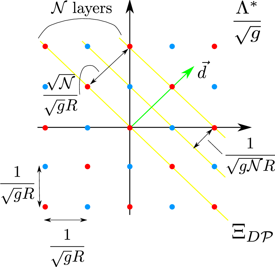
Now I determine , by calculating in two ways. First, since is the -dimensional hypercubic lattice with the lattice constant , we find
| (49) |
On the other hand, can be also written in terms of , as follows. The dimensional lattice is a intersection of and the hyperplane orthogonal to . This is illustrated in Fig. 4 for the simplest case of . The hypercubic lattice can be decomposed into parallel displacements of . Because is the simple cubic lattice with lattice constant , for any vector ,
| (50) |
with an integer . On the other hand, for any integer , there is always a vector which satisfies eq. (50). Eq. (50) represents the distance between the hyperplane and the origin. When eq. (50) holds, belongs to the -th parallel displacement of . Thus the distance between the neighboring hyperplanes hosting a copy of is
| (51) |
and the volume of the unit cell of the original lattice is given as
| (52) |
The denominator of eq. (6) corresponds to the amplitude of the -component free boson field theory with the boundary states and at the two ends. is the boundary state corresponding to
| (56) |
for . Namely, each field is identified with its “folding double” at the boundary. This corresponds to a boundary created by folding -component free boson in the bulk without any defect.
As I have discussed in Sec. 3, the boundary entropy for this artificially created “boundary” should be zero for any . Thus it must follow that
| (57) |
for any . In fact, eq. (57) for the boundary state can be also shown by an explicit calculation similar to that of . I note that, both and reduces to for ().
In the long cylinder limit , and I obtain
| (58) | ||||
| (59) |
Thus, using eq. (57), I find
| (60) |
in the long cylinder limit. The von Neumann entanglement entropy from the replica trick is thus given as
| (61) |
From eq. (55), for the quantum Lifshitz universality class,
| (62) |
To match the convention in Refs. [6, 7], I take and thus . This is different from the result reported in Ref. [6], by the second term . On the other hand, it indeed agrees exactly with that in Ref. [7] derived by different approaches. This shows that the basic ideas put forward in Refs. [5, 6] are correct, although care must be taken in changing the basis. Several results reported in Ref. [6] are not valid owing to negligence of the subtlety. The validity of the logarithmic term predicted in Ref. [5] will be discussed in Sec. 6.
5 Torus geometry
In Ref. [6], the entanglement entropy in the torus geometry was also discussed. Namely, a torus of total length is divided into two regions A and B of cylindrical shape. The boundary between A and B consists of two disjoint circles.

Again, for simplicity I consider the case and apply the folding trick to reduce the problem to -component free boson field theory on a cylinder of length , as in Fig. 5. By construction, in the present case, the “replica” boundary condition should be imposed on the both boundaries, in order to calculate the numerator of eq. (6). This is contrasted to the case of cylinder geometry discussed in Sec. 4, where the replica boundary condition is imposed at one end and the Dirichlet boundary condition at the other.
Thus I find
| (63) |
In the long cylinder limit,
| (64) |
This implies that
| (65) |
which leads to
| (66) |
This result is, again, different from that in Ref. [6]. In particular eq. (65) does not hold in Ref. [6]. On the other hand, eq. (65) is a general consequence of the boundary CFT, independent of the value of . In fact, although it was not explicitly discussed in Ref. [7], eq. (65) is also a general consequence of the mapping to classical statistical problem used in Ref. [7]. Thus the violation of the relation (65) is a clear signature of the problem in the calculation in Ref. [6].
I emphasize that eq. (65) does not hold for the entanglement entropy in general systems. It only applies to the critical wavefunction described as in eq. (2), for which the entanglement entropy can be related to classical (Shannon) entropy. [7] In fact, eq. (65) is violated in topological spin liquid phase.
6 Conclusion and Discussions
I have discussed the entanglement entropy in two-dimensional conformal critical points, in particular those described by free boson CFT (quantum Lifshitz universality class).
Calculations in Refs. [5, 6] were based on the fundamental formula (11) (or equivalently eq. (13)). However, there are two problems in this formula. First, in a general interacting theory, linear combinations of the original fields are not independent of each other as it was implicitly assumed in Refs. [5, 6]. On the other hand, CFTs other than the free boson field theory also admit free field representations. It might be used to extend the approach to general CFTs. However, it would be a nontrivial problem which requires further careful investigations.
Second, for the free boson field theory (which describes the quantum Lifshitz universality class), the bulk interaction is absent and the linear combinations appear independent. However, even in this case, they are not completely independent because of the intertwined compactification. I have demonstrated the importance of the nontrivial compactification using the simple example of single-component free boson field on a torus, which can be regarded as two-component free boson field with boundaries. “Mixed” Dirichlet/Neumann boundary conditions for general number of components, which appears in the replica trick calculation of the entanglement entropy, can be handled with a geometric formulation based on the compactification lattice. The constant part in the entanglement entropy corresponds to the universal boundary entropy in the CFT. This supports the universality of the constant term as proposed in Ref. [6]. In fact, the entanglement entropy obtained for the quantum Lifshitz universality class with the boundary CFT agrees exactly with that obtained with different methods in Ref. [7]. An incorrect value was reported in Ref. [6] because of the compactification was not properly taken into account.
The predictions made in Ref. [5] on the logarithmic term in eq. (1) should also be re-examined, since the fundamental formula (11), on which their derivation is based, does not hold as an exact identity. Nevertheless, their prediction on the logarithmic term could still stand valid for the following reason, in particular for the free boson (quantum Lifshitz) case. For the free boson field theory, in Ref. [5], they found the logarithmic term independent of the compactification radius. This suggests that the logarithmic term could be attributed solely to oscillator modes. For oscillator mode contributions, there is no subtlety discussed in the present paper and the “changing the basis” trick could be justified. From this perspective, it seems quite possible that their prediction on the logarithmic term is correct despite the subtle problem with eq. (11). It would mean that eq. (11) is valid in some restricted sense for determining the logarithmic term, although it is certainly not valid for determining the universal constant term. For general CFTs other than free boson, there is more problem in the “changing the basis” trick due to the bulk interaction. It might be still possible that the logarithmic term depends only on the central charge and the prediction in Ref. [5] is also valid for general CFTs, but it seems less convincing than in the free boson case, at this point.
In any case, in the present paper, I do not have any concrete result concerning the logarithmic term, and cannot draw a definitive conclusion about the prediction in Ref. [5] on the logarithmic term. I hope that the present paper will stimulate further progress in understanding of the logarithmic term.
It should be noted that the present paper, as well as the original work [6], is entirely based on (a simple implementation of) the replica trick. Its validity is by no means obvious. For the present case of free boson CFT, the agreement with different methods [7] implies that it is indeed valid. However, recently, its breakdown is suggested when the CFT corresponds to critical Ising model. [13] A general understanding of the issue is an important open problem.
Finally, when this paper was close to completion, a paper by Hsu and Fradkin has appeared [9]. There, they did not rely on eq. (13), which is not valid as I have discussed. Instead, they attempted to construct the boundary state in the spirit similar to the present paper. However, although their construction (eq. (14), or eq. (18) with eq. (19) of Ref. [9]) should give a consistent boundary state, it does not correspond to the required boundary condition (37) for the problem. As an indication, the condition (37) is invariant under any permutation of boson fields while their construction is not.
Furthermore, apparently there are several confusions in Ref. [9]. For example, in the original paper [6], as well as in Ref. [7] and in the present paper, the universal constant in the entanglement entropy was derived in the “long cylinder limit” (in the notation of the present paper). However, in Ref. [6], the definition of the lengths is somehow exchanged and the opposite limit is taken. As discussed in the present paper, in the long cylinder limit as introduced originally in Ref. [6], the universal constant part of the entanglement entropy should correspond to the universal boundary entropy (exponential of the groundstate degeneracy) in the boundary CFT.
Acknowledgements
I am grateful to Grégoire Misguich for introducing the problem to me, and for comments on the paper. I also thank Fabien Alet, Claudio Castelnovo, Michael Freedman, Shunsuke Furukawa, Joel Moore, Hirosi Ooguri, and Tadashi Takayanagi for useful discussions. This work is initiated at Laboratoire de Physique Théorique at IRSAMC Toulouse, and partially carried out at the International Workshop on Topological Order and Quantum Computation at Richard B. Gump South Pacific Research Station of UC Bekeley, and at the Summer Workshop “Low Dimensional Topological Matter” at Aspen Center for Physics.
This work is supported in part by Grant-in-Aid for Scientific Research on Innovative Areas No. 20102008 from MEXT of Japan, and by Grant-in-Aid for Challenging Exploratory Research No. 20654030 from JSPS.
Appendix A Boundary CFT of multicomponent boson field
In this Appendix, I summarize the relevant formulae in the boundary CFT of multicomponent compactified free boson field theory.
The boundary CFT was largely developed by Cardy [14, 15]. The development of boundary CFT of free boson field theory was also started in the context of string theory [16, 17], and continued for example in Refs. [18, 19, 20, 12]. For a review in the string theory context, see Refs. [21].
On the other hand, the boundary CFT is also relevant for some problems in condensed matter physics, such as quantum impurity problems and junction of one-dimensional quantum systems. The boundary CFT of free boson field theory is applied to impurities in quantum spin chains by Eggert and Affleck [22]. The boundary CFT of multicomponent free boson is applied to impurities in quantum wires by Wong and Affleck [8], and further discussed in related problems [23, 24, 10]
The multicomponent free boson field theory is defined by the Lagrangian density
| (67) |
where is a -dimensional vector.
I introduce the multidimensional generalization of the boson compactification as
| (68) |
where for a Bravais lattice , which is called as compactification lattice. For independent copies of the single-component boson compactified as in eq. (17), the compactification lattice is simply a hypercubic lattice with lattice constant . However, it is useful to formulate allowing more general compactification lattice.
I note that, as in the single-component case, the coupling constant can be set to any value by renormalizing the field , which also renormalize the compactification lattice. Thus is a redundant parameter once I consider general compactification lattice. Nevertheless, I keep the coupling constant for purpose of comparison as I have discussed for the single-component case. On the other hand, for general compactifications, it is impossible to fix the compactification lattice by renormalizing within the Lagrangian density of the form (67).
If we define the theory (67) on a finite length with the periodic boundary condition, the canonically quantized operator is given by the mode expansion
| (69) |
where . represents the winding number of when goes around the system. The canonical commutation relation of with the conjugate momentum field implies
| (70) |
Since the constant part is also subject to the compactification as in eq. (68), the eigenvalues of the conjugate “momentum” operator is quantized as
| (71) |
where belongs to the dual lattice , which is defined as a set of all ’s which satisfies
| (72) |
for any . The momentum operator in eq. (69) is often rewritten using eq. (71). However, it should be kept in mind that represents the eigenvalue of as in eq. (71).
The boson field can be decomposed into left-moving and right-moving components as
| (73) |
We can introduce the dual boson field as
| (74) |
From eq. (69), mode expansion of is given as
| (75) |
In this expression, the roles of and are interchanged compared to the mode expansion of in eq. (69). This implies that the dual field obeys compactification
| (76) |
where . is now interpreted as the eigenvalue of the dual “momentum” operator, which obeys canonical commutation relation similar to eq. (70) with the operator .
The Lagrangian density (67) can be also written in terms of as
| (77) |
Although and are mutually non-local, construction of a complete set of physical operators requires both and .
When we take boundary of a dimensional field theory orthogonal to the (imaginary) time axis, the boundary condition can be represented by the initial (or final) state. This is called as boundary state and is useful in systematic study of boundary conditions. In fact, nontrivial boundary conditions often cannot be defined precisely without introducing the boundary states. When the boundary condition is conformally invariant, the corresponding boundary state satisfies
| (78) |
for any integer , where are generators of the Virasoro algebra. For the multicomponent boson field, the Virasoro generators are given as
| (79) | ||||
| (80) |
where
Here each component of is a boson annihilation operator, , and . and their Hermitian conjugates (boson creation operators) represent the oscillator modes, corresponding to the quantized normal mode oscillations. These oscillator modes do not depend on the compactification. On the other hand, represent zero modes which are affected by the compactification.
The general solution of the conformal invariant boundary state (78) for the multicomponent free boson is not known. However, a sufficient condition for eq. (78) can be given as
| (87) |
for arbitrary integer . Here is an orthogonal matrix independent of . Eq. (87) for determines the boundary state to be of the form
| (88) |
where is an oscillator vacuum. This is a free boson version of Ishibashi state [25], which is conformal invariant.
In fact, there is an infinite number of oscillator vacua characterized by the zero mode quantum numbers. Following Ref. [10], I label these vacua as
| (89) |
and can be interpreted as the “winding numbers” of and of its dual , respectively, along the boundary. The Ishibashi state obtained as eq. (88) from eq. (89) is denoted as
| (90) |
Eq. (87) for puts a restriction on the vacua which can appear in the boundary state. That is, the quantum numbers must satisfy
| (91) |
For given orthogonal matrix , generally there is an infinite number of solutions which satisfy this requirement. Any linear combination of the Ishibashi states built from these vacua satisfies the conformal invariance (78).
However, a physical boundary state must also satisfy Cardy’s consistency condition, stated as follows. For a pair of given boundary conditions A and B, we can define the amplitude (partition function)
| (92) |
where By modular transformation, we can express this amplitude as a function of ,
| (93) |
where is a character of the Virasoro algebra. Since can be interpreted as the number of primary fields with conformal weight , it has to be a non-negative integer. This is Cardy’s consistency condition. Usually it is also required that , where corresponds to the identity operator. If one takes just a single Ishibashi state, Cardy’s condition cannot be satisfied. Generally, we take linear combination of Ishibashi states for all the zero modes allowed by eq. (91). It is also possible to construct consistent boundary states using only subset of zero modes allowed by eq. (91). However, those boundary states are more unstable and the most stable boundary states for a given turns out to be linear combinations of all the allowed zero mode vacua [10].
For example, taking gives Dirichlet boundary state. The solution of eq. (91) for is given by . Thus the Dirichlet boundary state is given as
| (94) |
where the summation in is taken over the entire dual lattice , and is a constant -dimensional vector. (There is an unfortunate conflict of notation; here is the coefficient of the boundary state and is a completely different quantity from the coupling constant defined in eq. (16).)
Physically, the constant vector corresponds to the boundary value of the field . This can be seen as follows. Let us consider the operator
| (95) |
where is a constant vector belonging to the dual lattice . This is a unique valued operator under the compactification 68. We apply this operator to the boundary state (94) at (imaginary) time . With respect to oscillator modes, each Ishibashi state constructed as in eq. (88) is a kind of coherent state. We observe that, for general ,
| (96) |
For the Dirichlet boundary condition, and thus applying the oscillator part of to the Ishibashi state yields zero. The winding number is zero in all the Ishibashi states in the boundary state (94), and at , contribution of the “momentum” eigenvalue to vanishes. Thus we find
| (97) |
Now the commutation relation (70) implies
| (98) |
Combining this with eq. (97), we find the eigenequation
| (99) |
This proves that can indeed be interpreted as the boundary value of the field . The Dirichlet boundary state is actually a continuous family of boundary states parametrized by . By symmetry, physical properties such as boundary entropy and scaling dimensions of the boundary operators are independent of . Thus the boundary value is often set to zero for simplicity. I denote simply by .
The Dirichlet-Dirichlet amplitude is given as
| (100) |
where
| (101) | ||||
| (102) |
Here is a Bravais lattice and is its dual, is the volume of the unit cell of the lattice , and
| (103) |
is the Dedekind eta function. I note that
| (104) |
Equality between eq. (101) and eq. (102) holds thanks to the multidimensional generalization of Poisson summation formula.
The coefficient in eq. (101) is fixed so that the amplitude in the form (102) satisfies Cardy’s consistency condition.
By comparison to eq. (101), we find
| (105) |
where is the volume of the unit cell of the compactification lattice . can be interpreted as universal non-integer groundstate degeneracy; in other words, is the boundary entropy for the Dirichlet boundary state.
Likewise, the Neumann boundary condition corresponds to . The Neumann boundary condition for is equivalent to the Dirichlet boundary condition for the dual field . The Neumann boundary state is given as
| (106) |
where is the boundary value of the dual field . The Neumann-Neumann amplitude reads
| (107) |
It follows that the groundstate degeneracy is
| (108) |
The Dirichlet-Neumann amplitude is also of interest; it must satisfy Cardy’s consistency condition as well. I note that, the Hamiltonian time evolution does not change the winding numbers from those in the initial state. Thus the only oscillator vacuum which contributes to the amplitude is , and no summation over zero modes appears in the Dirichlet-Neumann amplitude. The amplitude is thus given only by oscillator mode contributions as
| (109) |
where
| (110) |
is the Dirichlet-Neumann amplitude for a single component boson. Here are Jacobi’s theta function defined as
| (111) | ||||
| (112) |
This amplitude indeed satisfies Cardy’s consistency condition, as it should. It is also noted that this amplitude does not depend on the compactification.
Appendix B Construction of the boundary state for the simple example based on the gluing condition
Here I construct the boundary state for the boundary condition (21), using explicitly the gluing conditions (32) and (35). Although the boundary state can be given by a more systematic geometric formulation as in Sec. the present construction would be instructive to understand the importance of the gluing conditions.
As I have discussed in Sec. 3, the relevant boundary condition would correspond to the Dirichlet boundary condition for , namely , and the Neumann boundary condition for . The latter is equivalent to the Dirichlet boundary condition for the dual field, . Following the standard construction of the Dirichlet/Neumann boundary state for a free boson field theory, I can write down an ansatz:
| (113) |
where is the Ishibashi state with the winding numbers along the boundary
| (114) | ||||
| (115) |
where . The gluing conditions (32) and (35) imply, because , that and must be even integers. Thus the partition function (the amplitude with boundary state at the both ends) reads
| (116) |
Modular transforming, I obtain
| (117) |
which implies due to the Cardy’s consistency condition. Namely, there is no “boundary entropy” for this boundary, as it is required by physical grounds. Moreover, the partition function indeed agrees exactly with the original expression (19).
References
- [1] Calabrese P and Cardy J 2004 JSTAT 2004 P06002
- [2] Kitaev A and Preskill J 2006 Phys. Rev. Lett. 96 110404
- [3] Levin M and Wen X G 2006 Phys. Rev. Lett. 96 110405
- [4] Rokhsar D S and Kivelson S A 1988 Phys. Rev. Lett. 61 2376–2379
- [5] Fradkin E and Moore J E 2006 Phys. Rev. Lett. 97 050404
- [6] Hsu B, Mulligan M, Fradkin E and Kim E A 2009 Phys. Rev. B 79 115421
- [7] Stéphan J M, Furukawa S, Misguich G and Pasquier V 2009 Phys. Rev. B 80 184421
- [8] Wong E and Affleck I 1994 Nucl. Phys. B 417 403 – 438
- [9] Hsu B and Fradkin E 2010 arXiv:1006.1361
- [10] Oshikawa M, Chamon C and Affleck I 2006 JSTAT 2006 P02008
- [11] Oshikawa M and Affleck I 1997 Nucl. Phys. B 495 533 – 582
- [12] Ooguri H, Oz Y and Yin Z 1996 Nucl. Phys. B 477 407 – 430
- [13] Stéphan J M, Misguich G and Pasquier V 2010 arXiv:1006.1361
- [14] Cardy J L 1984 Nucl. Phys. B 240 514 – 532
- [15] Cardy J L 1989 Nucl. Phys. B 324 581 – 596
- [16] Polchinski J and Cai Y 1988 Nucl. Phys. B 296 91 – 128
- [17] Callan C G, Lovelace C, Nappi C R and Yost S A 1988 Nucl. Phys. B 308 221 – 284
- [18] Callan C G, Klebanov I R, Ludwig A W W and Maldacena J M 1994 Nucl. Phys. B 422 417 – 448
- [19] Callan C G, Klebanov I R, Maldacena J M and Yegulalp A 1995 Nucl. Phys. B 443 444 – 464
- [20] Yegulalp A 1995 Nuclear Physics B 450 641 – 662
- [21] Di Vecchia P and Liccardo A 1999 arXiv:hep-th/9912161, arXiv:hep-th/9912275
- [22] Eggert S and Affleck I 1992 Phys. Rev. B 46 10866–10883
- [23] Affleck I, Oshikawa M and Saleur H 2001 Nucl. Phys. B 594 535 – 606
- [24] Chamon C, Oshikawa M and Affleck I 2003 Phys. Rev. Lett. 91 206403
- [25] Ishibashi N 1989 Mod. Phys. Lett. A 4 251 – 264