RM3-TH/10-16
NLO QCD bottom corrections
to Higgs boson production in the MSSM
G. Degrassia and P. Slavichb
a
Dipartimento di Fisica, Università di Roma Tre and INFN, Sezione di
Roma Tre
Via della Vasca Navale 84, I-00146 Rome, Italy
b LPTHE, 4, Place Jussieu, F-75252 Paris, France
We present a calculation of the two-loop bottom-sbottom-gluino contributions to Higgs boson production via gluon fusion in the MSSM. The calculation is based on an asymptotic expansion in the masses of the supersymmetric particles, which are assumed to be much heavier than the bottom quark and the Higgs bosons. We obtain explicit analytic results that allow for a straightforward identification of the dominant contributions in the NLO bottom corrections. We emphasize the interplay between the calculations of the masses and the production cross sections of the Higgs bosons, discussing sensible choices of renormalization scheme for the parameters in the bottom/sbottom sector.
1 Introduction
With the coming into operation of the Large Hadron Collider (LHC), a new era has begun in the search for the Higgs boson(s). At the LHC the main production mechanism for the Standard Model (SM) Higgs boson, , is the loop-induced gluon fusion mechanism [1], , where the coupling of the gluons to the Higgs is mediated by loops of colored fermions, primarily the top quark. The knowledge of this process in the SM includes the full next-to-leading order (NLO) QCD corrections [2, 3], the next-to-next-to-leading order (NNLO) QCD corrections [4] including finite top mass effects [5], soft-gluon resummation effects [6], an estimate of the next-to-next-to-next-to-leading order (NNNLO) QCD effects [7] and also the first-order electroweak corrections [8, 9, 10].
The Minimal Supersymmetric extension of the Standard Model, or MSSM, features a richer Higgs spectrum which consists of two neutral CP-even bosons , one neutral CP-odd boson and two charged scalars . The gluon-fusion process is one of the most important production mechanisms for the neutral Higgs bosons, whose couplings to the gluons are mediated by colored fermions and their supersymmetric partners. The gluon-fusion cross section in the MSSM is known at the NLO. The contributions arising from diagrams with squarks and gluons were first computed under the assumption of vanishing Higgs mass in ref. [11]. The complete top/stop contributions, including stop mixing and gluino effects, were computed under the same assumption in ref. [12], and the result was cast in a compact analytic form in ref. [13]. Later, more refined calculations aimed at the inclusion of the full Higgs-mass dependence. In particular, the full squark-gluon contribution is known in a closed analytic form [14, 15, 16], while the full quark-squark-gluino contribution has been computed in ref. [17] via a combination of analytic and numerical methods.
It should be stressed that, at least for the case of the light Higgs, the exact two-loop QCD Higgs-gluon-gluon amplitude is in general well approximated by the amplitude evaluated in the limit of neglecting the Higgs mass. The latter is much easier to compute and the corresponding result can be straightforwardly implemented in computer codes that aim to evaluate the Higgs boson production cross section in a fast and efficient way. Indeed, it was noticed several years ago for the SM case [18] that the exact factor, defined as the ratio between the NLO and leading-order (LO) cross sections, is well approximated by the so-called effective factor that can be obtained via an improved effective-theory calculation. By the latter we mean a result in which the effective NLO cross section is obtained by multiplying the exact LO partonic cross section by the corrections evaluated in the limit of vanishing Higgs mass. For the SM case this approximation works at the level of few per cent for Higgs mass values below the threshold, and up to for any Higgs mass value. The same level of accuracy is reached when the Higgs couples to a generic scalar particle with mass , with the exception of a narrow region close to the threshold [19].
There is only one case in which the effective approximation does not work sufficiently well, namely when the bottom contribution becomes very relevant. This can happen in the MSSM when , i.e. the ratio of the vacuum expectation values (vev) of the neutral components of the two Higgs doublets, becomes large. In such a situation, in principle, the exact computation of the NLO bottom contribution to the cross section should be employed. However, explicit analytic results for the part of the NLO bottom contribution that is induced by two-loop bottom-sbottom-gluino diagrams have not been made available so far.
In this paper we present an approximate evaluation of the bottom-sbottom-gluino diagrams, based on an asymptotic expansion in the large supersymmetric masses that is valid up to and including terms of , and , where denotes a Higgs-boson mass and denotes a generic superparticle mass (). Together with the known exact results for the (s)bottom-gluon diagrams [3, 14, 15, 16, 19], our new result allows us to obtain effective factors that can be easily implemented in computer codes to provide an accurate and efficient evaluation of the cross section for Higgs boson production in the MSSM. Such factors are expected to be at the same level of accuracy as in the SM, i.e. within a few per cent of the exact value for the light Higgs and up to ten per cent for the heavy Higgs, with however a much better accuracy expected if the heavy-Higgs mass is below all the heavy-particle thresholds.
The paper is organized as follows: in section 2 we summarize general results on the cross section for Higgs boson production via gluon fusion. In section 3 we outline the way we perform the asymptotic expansion of the bottom-sbottom-gluino diagrams. Section 4 contains the explicit results for the NLO bottom contribution both in and in the on-shell (OS) scheme. In section 5 we discuss the numerical relevance of the NLO bottom corrections devoting particular attention to the interplay between the computation of the Higgs mass and that of its production cross section. In the last section we discuss an approximate way to take the NLO bottom contribution into account, based on an improved LO term. Finally, in appendix A we specialize to the MSSM case the general exact results for the real radiation derived in ref. [19], while appendix B contains the explicit expressions for the shifts from the to the OS parameters in the sbottom sector.
2 Higgs boson production via gluon fusion at NLO in the MSSM
In this section we recall for completeness some general results on Higgs boson production via gluon fusion. The hadronic cross section for Higgs boson production at center-of-mass energy can be written as
| (1) |
where , , is the factorization scale, the parton density of the colliding hadron for the parton of type (for ), and the cross section for the partonic subprocess at the center-of-mass energy . The latter can be written in terms of the LO contribution and a coefficient function as
| (2) |
We consider now the production of the lightest CP-even Higgs boson, , through gluon fusion11 1 For the heaviest eigenstate, , general formulae for the production cross section can be obtained straightforwardly with the replacements () in eqs. (3) and (17) and in appendix A.. The LO term can be written as
| (3) |
where is the muon decay constant, is the strong gauge coupling expressed in the renormalization scheme at the scale , is a color factor, and is the mixing angle in the CP-even Higgs sector of the MSSM. () are the form factors for the coupling of the neutral, CP-even component of the Higgs doublet with two gluons, which we decompose in one- and two-loop parts as
| (4) |
The one-loop form factors and contain contributions from diagrams involving quarks or squarks. The two-loop form factors and contain contributions from diagrams involving quarks, squarks, gluons and gluinos. Focusing on the contributions involving the third-generation quarks and squarks, and exploiting the structure of the Higgs-quark-quark and Higgs-squark-squark couplings, the form factors can be written to all orders in the strong interactions as [13]
| (5) | |||||
| (6) |
In the equations above and , where is the ratio of the vev of the two Higgs doublets. Also, is the higgsino mass parameter in the MSSM superpotential, (for ) are the soft SUSY-breaking Higgs-squark-squark couplings and are the left-right squark mixing angles (here and thereafter we use the notation for a generic angle ). The functions and appearing in eqs. (5) and (6) denote the contributions controlled by the third-generation Yukawa couplings, while denotes the contribution controlled by the electroweak, D-term-induced Higgs-squark-squark couplings. The latter can be decomposed as
| (7) |
where denotes the third component of the electroweak isospin of the quark , is the electric charge and is the Weinberg angle.
The one-loop functions entering and are:
| (8) | |||||
| (9) | |||||
| (10) |
where , and the functions and read
| (11) | |||||
| (12) |
The analytic continuations are obtained with the replacement . For later convenience, we recall the behavior of and in the limit in which the Higgs boson mass is much smaller or much larger than the mass of the particle running in the loop. In the first case, i.e. , which applies to the top and squark contributions for the light-Higgs case,
| (13) |
while in the opposite case, i.e. , which is relevant for the bottom quark,
| (14) |
The coefficient function in eq. (2) can be decomposed, up to NLO terms, as
| (15) |
with the LO contribution given only by the gluon-fusion channel:
| (16) |
The NLO terms include, besides the channel, also the one-loop induced processes and :
| (17) | |||||
| (18) |
where the LO Altarelli-Parisi splitting functions are
| (19) |
In the equations above, and ( being the number of colors), ( being the number of active flavors) is the one-loop -function of the strong coupling in the SM, and
| (20) |
The -channel contribution, eq. (17), involves two-loop virtual corrections to and one-loop real corrections from . The former, regularized by the infrared-singular part of the real emission cross section, are displayed in the first line of eq. (17). The second line contains the non-singular contribution from the real gluon emission in the gluon fusion process. The latter contribution as well as the ones due to the annihilation channel and the quark-gluon scattering channel, eq. (18), are obtained from one-loop diagrams where only quarks or squarks circulate in the loop. General expressions for the functions can be found in ref. [19] (see also refs. [20, 21]). In appendix A we provide expressions in which the contribution of the bottom quark is kept exact while those of the top quark and of the squarks are evaluated in the limit of vanishing Higgs mass.
The two-loop top/stop contributions to the form factors entering eq. (17) are fully under control in the light-Higgs case. Typically, the mass ratios between the Higgs and the particles running in the loops allow for the evaluation of the relevant diagrams via a Taylor expansion in the Higgs mass, with the zero-order term in the series already a very good approximation of the full result. The case of the two-loop bottom/sbottom contributions is obviously different. In general, Taylor-expanded evaluations of the relevant diagrams are no longer viable, due to the presence of the light bottom quark in the loops. Thus, the diagrams must be evaluated either exactly or via an asymptotic expansion in a large mass or momentum.
In the following sections we present the result for the NLO bottom contribution, combining earlier results in the literature with our new calculation of the bottom-sbottom-gluino contribution. The latter has been obtained via an asymptotic expansion, retaining terms of , and .
3 Outline of the calculation
An exact analytic evaluation of the bottom-sbottom-gluino contribution to is, at the moment, beyond our computational ability. However, it is reasonable to assume that all of the supersymmetric particles are much heavier than the lightest Higgs boson and the bottom quark, and look for an approximate evaluation of the diagrams in terms of a small-momentum (large-mass) expansion. We follow this path by performing a large-mass expansion, assuming all the supersymmetric particles to be heavy but without requiring any specific hierarchy among them.
After generating the two-loop diagrams involving bottom, sbottom and gluino that contribute to the process with the help of FeynArts [22], we separate them in two classes: i) those that can be evaluated via an ordinary Taylor expansion in powers of , of which we keep only the term of order zero; ii) the diagrams that require an asymptotic expansion. We recall that a Taylor expansion of a two-loop diagram in the external momentum is viable for values of up to the first physical threshold. In our case, diagrams with a physical threshold at , when Taylor-expanded in , exhibit an infrared (IR) divergent behavior as the bottom mass is sent to zero. Thus, these diagrams belong to the class ii.

Class-i diagrams are expressed in terms of two-loop vacuum integrals that can be evaluated using the results of ref. [23]. Concerning the diagrams belonging to class ii, reviews of the method of asymptotic expansions of Feynman diagrams with respect to masses or momenta can be found in ref. [24]. In practice, we generate the expansion of a diagram by adding and subtracting to it the part of the diagram itself that becomes IR-divergent when and are sent to zero. Formally we are adding nothing to the original diagram but, as graphically22 2 The diagrams have been drawn using JaxoDraw [25]. exemplified in fig. 1, this construction allows us to separate the diagram in two parts: part A in fig. 1 which, being by construction IR-safe, can be evaluated via a Taylor expansion in the same way as class-i diagrams; part B in fig. 1, containing the IR-divergent contribution, which should be evaluated exactly.
The IR-divergent part of a diagram is constructed in the following way. We first note that in all the diagrams entering our calculation one can choose a routing of momenta such that the connecting propagators, i.e. the propagators that contain both integration momenta and , are always accompanied by a heavy mass . Furthermore, only one subintegration, let us assume the one on , is IR divergent. Then, one can rewrite the connecting propagators using the identity
| (21) |
The first term on the r.h.s. of eq. (21) leads to a disconnected integral (product of two one-loop integrals) that contains the IR-divergent contributions present in the original diagram. This term can be evaluated exactly, i.e. for arbitrary , giving rise to the terms that describe the physical threshold. The second term, instead, leads to a two-loop integral with improved infrared convergence in the integration and improved ultraviolet convergence in the integration. Therefore, if, for example, the original integral is logarithmically IR divergent in the integration when and , the corresponding two-loop integral associated with the second term in eq. (21) evaluated at is no longer IR divergent, but it actually gives a finite result that differs from the result valid for and by terms of , where denotes either or . In general, a repeated application of eq. (21), controlled by the power counting in the IR-divergent terms, allows us to construct the IR-divergent part of any diagram in terms of products of one-loop integrals with numerators that contain terms of the form where are generic powers. The Passarino-Veltman reduction method is then applied to eliminate the numerators and express the result in terms of the known one-loop scalar integrals [26]. A check of the validity of our construction of the IR-divergent part of a diagram is given by the evaluation of its part A. Indeed, one verifies explicitly that the IR-divergent contributions of the original diagram are canceled by the terms constructed via eq. (21), so that the final result for part A is free of any or term.
4 Two-loop bottom/sbottom contributions
In this section we present the result for the two-loop bottom/sbottom contribution to the form factor for Higgs boson production via gluon fusion. We stress that, in the MSSM, the result for the production cross section of a Higgs boson is strictly linked to the computation of its mass, i.e., both observables should be computed in terms of the same set of SUSY parameters, defined in the same way beyond tree level. There is however an important difference between the two calculations. In the computation of the one-loop corrections to the Higgs masses, the diagrams involving the bottom quark are suppressed by the bottom mass and can be safely neglected, resulting in a one-loop contribution that is actually due to the sbottom diagrams only. This implies that in the two-loop calculation of the Higgs masses the only couplings that require a one-loop renormalization are the trilinear sbottom-Higgs couplings, while the definition of the bottom-Higgs Yukawa coupling beyond tree level is irrelevant. On the other hand, in the one-loop calculation of the amplitude for Higgs production both the bottom-Higgs Yukawa coupling and the trilinear sbottom-Higgs couplings play a role, thus they both require a one-loop definition when the two-loop contributions are computed.


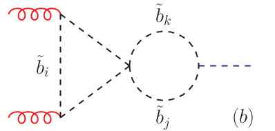

In the following we will discuss separately the contributions to the two-loop form factors from the diagrams involving the Higgs-bottom coupling (examples of which are shown in fig. 2) and those from the diagrams involving the Higgs-sbottom couplings (see fig. 3). In our approximation of neglecting terms beyond , the former contribute only to the function in eq. (5), while the latter contribute only to the functions and in eqs. (5) and (6). For both kinds of contributions, we first report the results obtained in the renormalization scheme, which is the scheme employed by several public computer codes [27] that return the MSSM mass spectrum starting from a set of high-energy boundary conditions for the SUSY-breaking parameters. We then discuss how to move from the scheme to a different renormalization prescription, which generalizes the one introduced for the calculation of the Higgs masses in ref. [28] and implemented in the code FeynHiggs [29]. With a slight abuse of language, since some of the amplitudes involved in the renormalization of the SUSY parameters are in fact evaluated off mass shell, we refer to this prescription as to the “on-shell” scheme.
4.1 Contributions controlled by the Higgs-bottom coupling
We start by considering the contributions of the two-loop diagrams involving the Higgs-bottom coupling. In our approximation those are the only diagrams that contribute to the function in eq. (5). The two-loop part of the function can be decomposed as
| (22) |
Assuming that the one-loop form factor is expressed in terms of -renormalized parameters evaluated at the scale , the contribution of the two-loop diagrams with bottom quarks and gluons (fig. 2a) reads:
| (23) |
Exact expressions for the functions , and are given in eqs. (2.12), (2.13) and (3.8) of ref. [15], respectively. In the limit they reduce to
| (24) | |||||
| (25) | |||||
| (26) | |||||
where and are Riemann’s zeta functions.
The contributions of the two-loop diagrams with bottom, sbottom and gluino (fig. 2b) require a dedicated calculation. Up to and including terms of and , and assuming that is expressed in terms of -renormalized parameters evaluated at the scale , they read:
| (27) | |||||
| (28) | |||||
where , and denotes the SUSY contribution to the bottom self-energy, in units of and in the limit of vanishing :
| (29) |
where
| (30) |
If the bottom-quark contribution to is expressed in terms of the pole bottom mass , the functions and are shifted with respect to their expressions in eqs. (23) and (27). In particular, the former becomes
| (31) |
and the term proportional to in the first line of eq. (27) is canceled out.
Eqs. (27) and (29) show that the bottom-sbottom-gluino contribution to contains terms enhanced by the large ratio . Recalling the definition of , it is clear that those terms are in fact of , i.e., they still vanish as but they are enhanced by the ratio . Such terms arise from two-loop diagrams in which the helicity flip on the fermion loop is achieved via a gluino mass insertion instead of a bottom mass insertion, and they by far dominate the new-physics contribution to the two-loop part of the form factors, no matter whether the bottom-quark contribution to is expressed in terms of the pole bottom mass or in terms of the -renormalized bottom mass . However, we notice that all of the two-loop terms cancel out if the one-loop bottom contribution to the function is computed in terms of , but the function itself is multiplied by instead of . As a result the function is further shifted, with respect to the expression corresponding to the use of in the whole one-loop contribution, by
| (32) |
This manipulation amounts to differentiating, in the one-loop contribution, between the parameter that describes the mass of the bottom quark running in the loop – which is identified with – and the parameter that describes the Yukawa coupling of the bottom quark to the Higgs boson – which is identified with . We recall that, in the MSSM, the running bottom mass can be related to the corresponding SM parameter as [30]
| (33) |
where denotes terms that are not enhanced by and, to ,
| (34) |
Since , it is easy to see that the terms enhanced by in do indeed contain . In the effective-theory language of ref. [31] we can argue that, by expressing the bottom Yukawa coupling entering in terms of as defined in eq. (33), we “resum” in the one-loop part of the form factor the -enhanced threshold corrections to the relation between the mass and the Yukawa coupling of the bottom quark. As a result of this special choice of parameters, all terms of the form drop out of the two-loop part of the form factor.
4.2 Contributions controlled by the Higgs-sbottom coupling
We now turn our attention to the diagrams that involve the Higgs-sbottom coupling. In our approximation those diagrams contribute only to the functions and in eqs. (5) and (6). In analogy with ref. [13], the two-loop parts of the functions can be written as
| (35) | |||||
| (36) | |||||
| (37) |
Furthermore, the various terms in eqs. (35)–(37) can be split in the contributions coming from diagrams with gluons (, fig. 3a), with strong, D-term-induced quartic bottom couplings (, fig. 3b), and with gluinos (, fig. 3c),
| (38) |
The first two terms in eq. (38) can be obtained from the analytic expressions presented for the stop contributions in eqs. (27)–(30) of ref. [13], identifying with after making the trivial replacement . The gluino contributions, on the other hand, require a dedicated calculation. Writing
| (39) |
and assuming that the parameters in and are expressed in the scheme at the renormalization scale , we find for the functions :
| (40) | |||||
| (41) | |||||
| (42) | |||||
| (43) |
where we retained only terms that induce , and contributions to . The expression for can be obtained from the expression for through the replacements and . Comparing eqs. (40) and (41) with eq. (42) of ref. [13] we notice that, contrary to what we stated in section 3.3 of that paper, even for the two-loop bottom-sbottom-gluino contribution to and cannot be obtained by taking the limit in the corresponding top contribution.
4.3 On-shell renormalization scheme for the sbottom parameters
We now discuss a suitable OS renormalization scheme for the parameters that determine the sbottom contribution to . We recall that, at the one-loop level, the vev and , the boson mass, the Weinberg angle and the parameter are not renormalized by the strong interactions. Therefore, the only parameters that require a one-loop definition are (), where by we denote the coupling constant entering the cubic and quartic sbottom-Higgs interactions, which at tree level is related to the bottom mass by . Indeed, the factor that multiplies the function in eqs. (5) and (6) has to be interpreted as a bookmark for . In fact, only four of those parameters are independent, because of the relation
| (44) |
In the analysis of the sbottom corrections to the neutral MSSM Higgs boson masses presented in ref. [28] it was pointed out that, while the sbottom masses can be naturally identified with the pole masses, an OS definition of is less easily singled out. Proceeding in analogy with the OS renormalization of the stop sector (see, e.g., ref. [13]), we might choose as independent parameters a conveniently defined bottom mixing angle, , and the bottom Yukawa coupling , as defined by the pole bottom mass via the relation . Then, eq. (44) might be used to establish the one-loop definition of in terms of the pole bottom and sbottom masses and the sbottom mixing angle. However, for large values of such definition would produce very large shifts in with respect to its value 33 3 For the generic parameter , we define the shift from the value as ., [32]. This is related to the fact that, in the large- limit (i.e., ), becomes independent of as can be easily seen from eq. (44). To cure the problem, it was suggested in ref. [28] (see also ref. [33]) to take and as independent parameters, while considering as a derived quantity via eq. (44). Suitable renormalization conditions were then proposed for and .
In the OS analysis of the cross section for Higgs boson production we want to retain the convenient features of the renormalization prescription employed in ref. [28]. However, that prescription needs to be expanded: first of all, the renormalization conditions in ref. [28] were defined in the limit (i.e., ), while in the case at hand we do not impose constraints on . Moreover, while in the calculation of the one-loop corrections to the Higgs masses the contributions controlled by the bottom-Higgs Yukawa coupling (which we denote as to distinguish it from ) are suppressed, the one-loop diagram controlled by gives an important contribution to the production cross section. Therefore, a one-loop definition of is required. Since it does not seem appropriate to define the bottom-Higgs coupling in terms of quantities of the sbottom sector, as would happen if we imposed on it the same renormalization condition used for , we need to impose different renormalization conditions on and , or, equivalently, on the bottom mass that enters the one-loop bottom contribution and the one that enters the one-loop sbottom contribution. In particular, we identify the former with the pole mass (the resulting shifts in the function are discussed in section 4.1). Concerning the bottom mass in the one-loop sbottom contribution, we follow ref. [28], extending the prescription presented in that paper to the case of finite .
To obtain definitions for and , we consider two quantities
| (45) |
that allow for a natural interpretation: , at the classical level, is the off-diagonal term in the sbottom mass matrix, related to the mixing angle via eq. (44); is proportional to the coefficient of the trilinear interaction . A definition of the mixing angle like the one proposed in ref. [34],
| (46) |
together with the identification of the sbottom masses as pole masses, can be immediately translated, using eq. (44), into a prescription for :
| (47) |
In eqs. (46) and (47), denotes the finite part of the self-energy of the sbottoms.
Recalling that in the limit , the extension to the case of finite of the prescription for introduced in eq. (15) of ref. [28] reads:
| (48) | |||||
where denotes the proper vertex .
Finally, the shifts of the parameters and are related to those of and by
| (49) | |||||
| (50) |
where . Explicit expressions for and , as well as for and , can be found in appendix B.
If the one-loop sbottom contribution to and is evaluated in terms of OS quantities, the two-loop functions in eqs. (35)–(37) must be replaced by
| (51) | |||||
| (52) | |||||
| (53) |
In addition, the two-loop form factor receives a contribution originating from the shift in :
| (54) |
5 A numerical example
We will now illustrate the effect of the two-loop bottom/sbottom contributions to the form factors for the production of a Higgs boson in a representative region of the MSSM parameter space.
The SM parameters entering our calculation are the boson mass GeV, the Fermi parameter GeV-2, the sine of the Weinberg angle and the strong coupling constant [35]. For the pole masses of the top and bottom quarks we take GeV [36] and GeV, the latter corresponding to the SM running mass (in the scheme) GeV [37]. The tree-level mass matrix for the CP-even Higgs bosons can be expressed in terms of the physical pseudoscalar mass and the -renormalized parameter , in addition to . In the calculation of the physical Higgs boson masses and of the mixing angle we include the one-loop and two-loop corrections as in refs. [28, 38].
When computing the two-loop corrections to both mass matrix and production form factors for the CP-even Higgs bosons, the parameters that determine the stop and sbottom masses and mixing angle and are subject to corrections require a one-loop specification. For the stop sector we adopt the OS scheme described e.g. in ref. [13]. In particular, we take as input the pole top mass and the soft SUSY-breaking parameters that can be derived by rotating the diagonal matrix of the OS stop masses by the angle , defined as in eq. (37) of ref. [13]. Concerning the corresponding parameters of sbottom sector additional care is required, because of our non-trivial definition of and of the fact that, at , the parameter entering the sbottom mass matrix differs from the corresponding stop parameter by a finite shift [32]. We start by computing the renormalized Higgs-sbottom coupling as given by , where is the -renormalized running coupling that can be trivially extracted from computed via eq. (33), and is defined in eq. (49). Then we compute following the prescription of [32]. Finally, we use the parameters and to compute the actual values of the OS sbottom masses and mixing angle.


To set the stage for further discussion, we show in fig. 4 the masses and mixing angle of the CP-even Higgs bosons as a function of . All the relevant SUSY-breaking parameters, as well as the supersymmetric mass parameter , are set to a common value = 500 GeV, and the physical pseudoscalar mass is set to 150 GeV. The left panel of fig. 4 shows the masses of the two Higgs bosons and in the range , while the right panel shows the combinations and , which determine the strength of the coupling of to the bottom and top quarks, respectively, relative to the corresponding SM couplings. For each set of curves, the solid line represents the result obtained in the OS renormalization scheme of ref. [28], described in section 4.3. For comparison, we also show as a dotted line the result that would be obtained if the sbottom parameters and were renormalized in the same way as the corresponding stop parameters. The left plot shows the well-known fact that, at large , the radiative corrections from sbottom loops tend to reduce . The right plot shows that, for the chosen values of and , the coupling of to the bottom quark is still substantially enhanced with respect to its SM value. This has to be contrasted with the couplings of to the top quark and to the gauge bosons (not shown), which are already very close to the SM values they tend to in the “decoupling” limit .
The comparison between the dotted and solid lines in fig. 4 shows that, if we had adopted for the sbottom parameters and the renormalization scheme used for the stop parameters, the results for and for would differ wildly from the ones obtained with the renormalization scheme discussed in section 4.3 (conversely, we checked that the results obtained in the scheme would be in good qualitative agreement with the solid lines). The discrepancy is due to the fact that in the “bad” OS scheme the (1,1) and (1,2) entries of the CP-even Higgs mass matrix are subject to very large two-loop corrections scaling like , induced by the contribution of the counterterm . It is interesting to note that, since the contribution of to the form factor in eq. (54) is suppressed by a factor , its impact on the Higgs boson production cross section in the “bad” OS scheme is not as extreme as the impact on the Higgs mass. However, we stress that a consistent determination of the properties of the Higgs bosons requires that the same definition of input parameters be used in the calculations of mass and production cross section. Since the naive choice of using the same OS renormalization scheme for the stop and sbottom sectors is not viable in the calculation of the Higgs masses, it should not be applied to the calculation of the cross section either.


We are now ready to discuss the effect of the two-loop bottom/sbottom contributions to the form factor for Higgs-boson production. To this purpose, we define a factor that contains the ratio of two-loop to one-loop form factors appearing in eq. (17):
| (55) |
In the left panel of fig. 5 we plot as a function of , with the same choice of SUSY parameters as in fig. 4, in the OS renormalization scheme described in section 4.3. The one-loop form factors in the denominator of the term between parentheses in eq. (55) contain both the top/stop and bottom/sbottom contributions, computed under the approximations of eqs. (13) and (14). The lines in the plot correspond to different computations of the two-loop form factors in the numerator: the dotted line includes only the contributions of the top/stop sector, as computed in ref. [13]; the dashed line includes also the contribution of two-loop diagrams with bottom quarks and gluons; the solid line includes the full two-loop contribution of the bottom/sbottom sector as computed in section 4; finally, the dot-dashed line is obtained by approximating the bottom/sbottom contribution (with the exception of the bottom-gluon diagrams) with just the terms enhanced by in eq. (27). From the comparison between the dotted and dashed lines it can be seen that, in the OS renormalization scheme, the contribution to of the two-loop diagrams with bottom quarks and gluons is very small. This is due to a partial cancellation between the terms and entering the function , and to the fact that, in this scheme, the term is not enhanced by the potentially large logarithm of the ratio between the bottom mass and the renormalization scale, as can be seen by comparing eqs. (23) and (31). The solid line shows that the effect of the diagrams involving sbottoms can be very sizable at large , more than doubling . Indeed, for large the coupling of the light Higgs boson to the (s)bottom is considerably enhanced with respect to its SM value, as can be seen in the right panel of fig. 4. However, the proximity between the solid and dot-dashed lines shows that this sizable effect is almost entirely due to the terms enhanced by in the contribution of the two-loop bottom-sbottom-gluino diagrams in which the light Higgs boson couples to the bottom quark.
As discussed in section 4.1, the terms enhanced by in the OS result can be canceled out if the Higgs-bottom Yukawa coupling in the one-loop part of the result is identified with the -renormalized MSSM bottom mass instead of the physical mass . To this effect, the factor multiplying the function in eq. (5) must be expressed as , and the two-loop part of must be shifted as in eq. (32). In the right panel of fig. 5 we present the result of this manipulation, with evaluated at the scale . The input parameters and the meaning of the different lines are the same as for the plot in the left panel. The proximity between the dashed and solid lines shows that the contribution of the two-loop diagrams involving sbottoms is rather small in this renormalization scheme, at least for our choice of input parameters. However, still shows a sizable increase at large . This is due to the fact that the shift in eq. (32) brings back a large logarithm, , in the contribution of the two-loop diagrams with bottom and gluon (this logarithm compensates the scale dependence of the running mass ).


To conclude this section, we show in fig. 6 the factor for the production of the heavy CP-even Higgs boson, in the range . The definition of can be obtained from the one of in eq. (55) via the replacements . The input parameters are chosen exactly as in figs. 4 and 5, and the meaning of the lines in the left and right panels is the same as in fig. 5. Since in this example the mass of the heavy Higgs boson is of the order of 150 GeV (see fig. 4), i.e. well below any threshold for heavy-particle production, we expect the approximation of vanishing Higgs mass to hold reasonably well even for . From fig. 6 it appears that the balance of the various contributions to in the two different renormalization schemes is qualitatively similar to the one for shown in fig. 5: in the OS scheme the factor receives a sizable contribution from the sbottom diagrams, largely dominated by the terms enhanced by in the diagrams controlled by the Higgs-bottom coupling; in the “mixed” scheme, on the other hand, the sbottom contribution is rather small, but there is a sizable contribution from the diagrams with bottom and gluon.
This said, the factor shows a peculiar dependence on : for sufficiently large values of , it grows linearly in the OS scheme, while it reaches a plateau in the mixed scheme. This can be easily understood by recalling that, for moderate-to-large and for our choice of , the Yukawa coupling of the heavy MSSM Higgs to bottom quarks is enhanced by with respect to the SM value, while the coupling to top quarks is suppressed by . Consequently, both the one-loop and the two-loop form factors in are dominated by the contribution of the diagrams controlled by the Higgs-bottom coupling, with the result that the coupling itself cancels out in the ratio. However, the dominant contribution from the bottom-sbottom-gluino diagrams in the OS scheme contains an additional -enhancement hidden in the product (see the discussion at the end of section 4.1), which explains the linear rise of . On the other hand, the dominant contribution of the bottom-gluon diagrams in the mixed scheme possesses no further -enhancement, which explains the plateau.
6 Conclusions and discussion
In this paper we presented analytic results for the NLO bottom-sbottom-gluino contribution to the cross section for Higgs boson production in gluon fusion, obtained using an asymptotic expansion in the large supersymmetric masses. This approximation is fully valid for the light-Higgs case, while for the heavy Higgs it covers the mass region where is below all the heavy-particle thresholds. Together with the previously known results for the NLO corrections in the MSSM, our expressions can be easily implemented in computer codes that aim to provide an accurate and efficient evaluation of the cross section for Higgs boson production in the MSSM.
In our analysis we paid special attention to the consistency between the calculations of the masses and the production cross sections of the MSSM Higgs bosons, i.e. to the fact that the same input parameters, defined at the one-loop level, should be used in both calculations. The OS definition of the parameters of the bottom sector is delicate, as discussed for the case of the Higgs masses in ref. [28]. The choice of treating the top and the bottom sectors on the same footing suffers from the fact that large two-loop corrections proportional to are generated in the contributions controlled by the Higgs-sbottom couplings, affecting both the calculation of the Higgs masses and that of the production cross sections. To avoid such large two-loop effects, a convenient OS renormalization prescription was proposed in ref. [28] for the calculation of the Higgs masses. In the present paper we have extended that prescription to cover also the calculation of the production cross sections.
Our analysis of the NLO bottom contribution to the gluon-fusion production cross section shows that, with our choice of OS renormalization conditions, the bulk of the corrections comes from the two-loop diagrams involving the Higgs-bottom Yukawa coupling, while the diagrams controlled by the Higgs-sbottom coupling play a secondary role. The contribution controlled by the Higgs-bottom Yukawa coupling can be further divided in two parts: diagrams with only bottom and gluons and diagrams involving bottom, sbottom and gluino. By far, the most important pieces of the latter diagrams are the terms of , i.e. the ones in which the helicity flip on the fermion line is achieved via a gluino mass insertion instead of a bottom mass insertion.
It is natural to wonder if it is possible to absorb most of the NLO bottom contribution into the LO term with a suitable choice of the input parameters. In such a situation the factor , as defined in eq. (55), would be basically sensitive to the top/stop contribution only. The contribution of the two-loop bottom-gluon diagrams can be made small if the one-loop bottom diagrams are expressed in terms of the pole bottom mass , but in this case the terms give a sizable contribution. On the other hand, if the Higgs-bottom Yukawa coupling in the one-loop result is expressed in terms of the running bottom mass , and the bottom mass in terms of , the terms in the two-loop contribution cancel out, but the bottom-gluon diagrams give a relevant contribution because of the presence of large logarithms of the ratio between and the renormalization scale. However, the explicit knowledge of the NLO bottom contribution allows us to devise a simple recipe to absorb the bulk of the NLO contribution into the LO term. It amounts to writing the LO bottom contribution entirely in terms of the pole bottom mass , then rescaling it by a factor . Once this manipulation is implemented, we expect the remaining NLO bottom/sbottom contributions to be quite small – at least in large regions of the parameter space – in which case they can be neglected in the evaluation of the form factors without introducing large errors44 4 A somewhat similar procedure was suggested, without a detailed discussion, in ref. [39].. We stress that the validity of this simple recipe is strictly linked to the absence of spuriously large corrections to the Higgs-sbottom coupling. This is realized with our choice of OS renormalization conditions for the sbottom sector (and also in the scheme) but it is not guaranteed with other renormalization conditions.
Finally, the results derived in this paper for the production cross section can be straightforwardly applied to the NLO computation of the gluonic and photonic decay widths of the CP-even Higgs boson in the MSSM, as described in section 5 of ref. [13].
Acknowledgments
This work was supported in part by an EU Marie-Curie Research Training Network under contract MRTN-CT-2006-035505 (HEPTOOLS) and by ANR under contract BLAN07-2_194882.
Appendix A: NLO contributions from real parton emission
In this appendix we specialize to the MSSM case the general exact results of ref. [19] for the functions . We aim at expressions that, on one hand, are sufficiently accurate, while on the other hand allow for a fast numerical evaluation. Thus we report expressions in which the contributions of the top quark and of the squarks are evaluated in the limit of neglecting the Higgs mass, while the contribution of the bottom quark is kept exact.
The function can be written as
| (A1) |
where , with
| (A2) |
Furthermore, the functions and can be cast in the following form:
| (A3) | |||||
| (A4) |
with
| (A6) | |||||
| (A7) | |||||
| (A8) |
where the functions and are defined in eqs. (2.22) and (2.24) of ref. [19], respectively, and it is understood that the top and squark contributions to are evaluated in the limit of neglecting the Higgs mass. In several cases the terms proportional to in eqs. () and (A7) are numerically very small and can be neglected. In such a situation the integration in eq. (A1) can be performed analytically, resulting in .
The annihilation channel can be written as
| (A9) |
with
| (A10) |
where
| (A11) | |||||
| (A12) |
The function is defined in eq. (2.31) of ref. [19].
Finally, we consider the quark-gluon scattering channel, . The relevant function can be written as
where
| (A14) |
As in the case of , when the terms proportional to in eq. (A11) can be neglected the integration in eq. () can be performed analytically, giving and .
Appendix B: Renormalization scheme shifts in the sbottom sector
In this appendix we present explicit expressions for the shifts from the to the OS scheme of the parameters in the sbottom sector that require a one-loop definition. Denoting, generically, a quantity in the scheme as , and the same quantity in the OS scheme as , we can write the one-loop relation as . Retaining only terms that do not induce contributions suppressed by , we find:
| (B1) | |||||
| (B2) | |||||
| (B3) | |||||
| (B4) |
where the notation in eqs. (B3) and (B4) means a term that is obtained from the previous ones inside the square bracket with the exchange . The shift is obtained from eq. (B1) via the interchange . Finally we note that the expressions for and in eq. (B3) and eq. (B4), respectively, which are valid for generic values of , coincide with the corresponding expressions in ref. [28], which were derived in the limit .
References
- [1] H. M. Georgi, S. L. Glashow, M. E. Machacek and D. V. Nanopoulos, Phys. Rev. Lett. 40 (1978) 692.
- [2] S. Dawson, Nucl. Phys. B 359 (1991) 283; A. Djouadi, M. Spira and P. M. Zerwas, Phys. Lett. B 264 (1991) 440.
- [3] M. Spira, A. Djouadi, D. Graudenz and P. M. Zerwas, Nucl. Phys. B 453 (1995) 17 [arXiv:hep-ph/9504378]; R. Harlander and P. Kant, JHEP 0512 (2005) 015 [arXiv:hep-ph/0509189].
- [4] R. V. Harlander, Phys. Lett. B 492 (2000) 74. [arXiv:hep-ph/0007289]; S. Catani, D. de Florian and M. Grazzini, JHEP 0105 (2001) 025 [arXiv:hep-ph/0102227]; R. V. Harlander and W. B. Kilgore, Phys. Rev. D 64 (2001) 013015 [arXiv:hep-ph/0102241], Phys. Rev. Lett. 88 (2002) 201801 [arXiv:hep-ph/0201206]; C. Anastasiou and K. Melnikov, Nucl. Phys. B 646 (2002) 220 [arXiv:hep-ph/0207004]; V. Ravindran, J. Smith and W. L. van Neerven, Nucl. Phys. B 665 (2003) 325 [arXiv:hep-ph/0302135].
- [5] S. Marzani, R. D. Ball, V. Del Duca, S. Forte and A. Vicini, Nucl. Phys. B 800 (2008) 127 [arXiv:0801.2544 [hep-ph]]; S. Marzani, R. D. Ball, V. Del Duca, S. Forte and A. Vicini, Nucl. Phys. Proc. Suppl. 186 (2009) 98 [arXiv:0809.4934 [hep-ph]]; R. V. Harlander and K. J. Ozeren, Phys. Lett. B 679 (2009) 467 [arXiv:0907.2997 [hep-ph]], JHEP 0911 (2009) 088 [arXiv:0909.3420 [hep-ph]]; A. Pak, M. Rogal and M. Steinhauser, Phys. Lett. B 679 (2009) 473 [arXiv:0907.2998 [hep-ph]], JHEP 1002 (2010) 025 [arXiv:0911.4662 [hep-ph]]; R. V. Harlander, H. Mantler, S. Marzani and K. J. Ozeren, Eur. Phys. J. C 66 (2010) 359 [arXiv:0912.2104 [hep-ph]].
- [6] S. Catani, D. de Florian, M. Grazzini and P. Nason, JHEP 0307 (2003) 028 [arXiv:hep-ph/0306211].
- [7] S. Moch and A. Vogt, Phys. Lett. B 631 (2005) 48 [arXiv:hep-ph/0508265]; V. Ravindran, Nucl. Phys. B 752 (2006) 173 [arXiv:hep-ph/0603041].
- [8] A. Djouadi and P. Gambino, Phys. Rev. Lett. 73 (1994) 2528 [arXiv:hep-ph/9406432]; A. Djouadi, P. Gambino and B. A. Kniehl, Nucl. Phys. B 523 (1998) 17 [arXiv:hep-ph/9712330].
- [9] U. Aglietti, R. Bonciani, G. Degrassi and A. Vicini, Phys. Lett. B 595 (2004) 432 [arXiv:hep-ph/0404071], Phys. Lett. B 600 (2004) 57 [arXiv:hep-ph/0407162]; G. Degrassi and F. Maltoni, Phys. Lett. B 600 (2004) 255 [arXiv:hep-ph/0407249].
- [10] S. Actis, G. Passarino, C. Sturm and S. Uccirati, Phys. Lett. B 670 (2008) 12 [arXiv:0809.1301 [hep-ph]], Nucl. Phys. B 811 (2009) 182 [arXiv:0809.3667 [hep-ph]].
- [11] S. Dawson, A. Djouadi and M. Spira, Phys. Rev. Lett. 77 (1996) 16 [arXiv:hep-ph/9603423].
- [12] R. V. Harlander and M. Steinhauser, Phys. Lett. B 574 (2003) 258 [arXiv:hep-ph/0307346], JHEP 0409 (2004) 066 [arXiv:hep-ph/0409010].
- [13] G. Degrassi and P. Slavich, Nucl. Phys. B 805 (2008) 267 [arXiv:0806.1495 [hep-ph]].
- [14] C. Anastasiou, S. Beerli, S. Bucherer, A. Daleo and Z. Kunszt, JHEP 0701 (2007) 082 [arXiv:hep-ph/0611236].
- [15] U. Aglietti, R. Bonciani, G. Degrassi and A. Vicini, JHEP 0701 (2007) 021 [arXiv:hep-ph/0611266].
- [16] M. Muhlleitner and M. Spira, Nucl. Phys. B 790 (2008) 1 [arXiv:hep-ph/0612254].
- [17] C. Anastasiou, S. Beerli and A. Daleo, Phys. Rev. Lett. 100 (2008) 241806 [arXiv:0803.3065 [hep-ph]].
- [18] M. Kramer, E. Laenen and M. Spira, Nucl. Phys. B 511, 523 (1998) [arXiv:hep-ph/9611272].
- [19] R. Bonciani, G. Degrassi and A. Vicini, JHEP 0711 (2007) 095 [arXiv:0709.4227 [hep-ph]].
- [20] R. K. Ellis, I. Hinchliffe, M. Soldate and J. J. van der Bij, Nucl. Phys. B 297 (1988) 221.
- [21] U. Baur and E. W. N. Glover, Nucl. Phys. B 339 (1990) 38.
- [22] T. Hahn, Comput. Phys. Commun. 140 (2001) 418 [arXiv:hep-ph/0012260]; T. Hahn and C. Schappacher, Comput. Phys. Commun. 143 (2002) 54 [arXiv:hep-ph/0105349].
- [23] A. I. Davydychev and J. B. Tausk, Nucl. Phys. B 397 (1993) 123.
- [24] V. A. Smirnov, Springer Tracts Mod. Phys. 177 (2002) 1; V. A. Smirnov and E. R. Rakhmetov, Theor. Math. Phys. 120 (1999) 870 [Teor. Mat. Fiz. 120 (1999) 64] [arXiv:hep-ph/9812529].
- [25] D. Binosi and L. Theussl, Comput. Phys. Commun. 161 (2004) 76 [arXiv:hep-ph/0309015].
- [26] G. Passarino and M. J. G. Veltman, Nucl. Phys. B 160 (1979) 151.
- [27] B. C. Allanach, Comput. Phys. Commun. 143, 305 (2002) [arXiv:hep-ph/0104145]; A. Djouadi, J. L. Kneur and G. Moultaka, Comput. Phys. Commun. 176, 426 (2007) [arXiv:hep-ph/0211331]; W. Porod, Comput. Phys. Commun. 153, 275 (2003) [arXiv:hep-ph/0301101].
- [28] A. Brignole, G. Degrassi, P. Slavich and F. Zwirner, Nucl. Phys. B 643, 79 (2002) [arXiv:hep-ph/0206101].
- [29] S. Heinemeyer, W. Hollik and G. Weiglein, Comput. Phys. Commun. 124 (2000) 76 [arXiv:hep-ph/9812320].
- [30] L. J. Hall, R. Rattazzi and U. Sarid, Phys. Rev. D 50 (1994) 7048 [arXiv:hep-ph/9306309].
- [31] M. S. Carena, D. Garcia, U. Nierste and C. E. M. Wagner, Nucl. Phys. B 577 (2000) 88 [arXiv:hep-ph/9912516].
- [32] A. Bartl, H. Eberl, K. Hidaka, T. Kon, W. Majerotto and Y. Yamada, Phys. Lett. B402 (1997) 303 [hep-ph/9701398]; H. Eberl, K. Hidaka, S. Kraml, W. Majerotto and Y. Yamada, Phys. Rev. D62 (2000) 055006 [hep-ph/9912463].
- [33] S. Heinemeyer, W. Hollik, H. Rzehak and G. Weiglein, Eur. Phys. J. C 39 (2005) 465 [arXiv:hep-ph/0411114]; S. Heinemeyer, H. Rzehak and C. Schappacher, arXiv:1007.0689 [hep-ph].
- [34] A. Pilaftsis, Nucl. Phys. B 504 (1997) 61 [arXiv:hep-ph/9702393]; J. Guasch, J. Sola and W. Hollik, Phys. Lett. B 437 (1998) 88 [arXiv:hep-ph/9802329]; H. Eberl, S. Kraml and W. Majerotto, JHEP 9905 (1999) 016 [arXiv:hep-ph/9903413]; Y. Yamada, Phys. Rev. D 64 (2001) 036008 [hep-ph/0103046].
- [35] C. Amsler et al. [Particle Data Group], Phys. Lett. B 667 (2008) 1.
- [36] [Tevatron Electroweak Working Group and CDF Collaboration and D0 Collab], arXiv:0903.2503 [hep-ex].
- [37] J. H. Kuhn, M. Steinhauser and C. Sturm, Nucl. Phys. B 778 (2007) 192 [arXiv:hep-ph/0702103]; K. G. Chetyrkin, J. H. Kuhn, A. Maier, P. Maierhofer, P. Marquard, M. Steinhauser and C. Sturm, Phys. Rev. D 80 (2009) 074010 [arXiv:0907.2110 [hep-ph]]; J. H. Kuhn, arXiv:1001.5173 [hep-ph].
- [38] G. Degrassi, P. Slavich and F. Zwirner, Nucl. Phys. B 611 (2001) 403 [arXiv:hep-ph/0105096].
- [39] M. Muhlleitner, H. Rzehak and M. Spira, arXiv:1001.3214 [hep-ph].