Multiple Scattering: Dispersion, Temperature Dependence, and Annular Pistons
Abstract
We review various applications of the multiple scattering approach to the calculation of Casimir forces between separate bodies, including dispersion, wedge geometries, annular pistons, and temperature dependence. Exact results are obtained in many cases.
1 Quantum Vacuum Energy
Quantum vacuum energies, or Casimir energies, are important at all energy scales, from subnuclear to cosmological. Applications are starting to appear in nanotechnology. Furthermore it is most likely that the source of dark energy that makes up some 70% of the energy budget of the universe is quantum vacuum fluctuations. In particular, the 7-year WMAP data is completely consistent with the existence of a cosmological constant [1],
| (1) |
which is precisely what would be expected if dark energy arose from this source [2]. Finally, zero-point fluctuations may be the most fundamental aspect of quantum field theory.
2 Multiple-Scattering Formulation
The multiple scattering formulation is easiest stated for a scalar field, which is rather ‘easily’ generalized to electromagnetism. For example, see Ref. [3]. Vacuum energy is given by the famous trace-log formula,
| (2) |
where in terms of the background potential ,
| (3) |
Now we define the -matrix,
| (4) |
and if the potential has two disjoint parts, , it is easy to derive the interaction between the two bodies (potentials):
| (5a) | |||||
| (5b) | |||||
where , , and likewise refers to .
3 Quantum Vacuum Energy—Dispersion
Perhaps not surprisingly in retrospect, we find that the usual dispersive form of the electromagnetic energy [4]
| (6) |
must be used, which, quantum mechanically, corresponds to the vacuum energy form
| (7) |
in terms of the Green’s dyadic . This result follows directly from the trace-log formula for the vacuum energy
| (8) |
and is equivalent to the variational statement [5]
| (9) |
From the energy, precisely because the dispersive derivative terms are present, we recover the Lifshitz formula for the energy per area between parallel dielectric slabs, with permittivity , separated by a medium of permittivity of thickness ,
| (10) |
with , being the imaginary frequency. The TE reflection coefficients are given by
| (11) |
while the TM coefficients are obtained from these by the substitution . For further details of this calculation, see Ref. [6].
4 Noncontact Gears
The program of calculating the quantum vacuum lateral force between corrugated surfaces and gears has been under active development. The electromagnetic situation of currugated dielectric slabs is illustrated in Fig. 1. For details see Ref. [7].
[width=70mm,scale=1.0] corru-new.ps
In the conductor limit () and for the case of sinusoidal corrugations described by and the lateral force can be evaluated to be in first order in and
| (12) |
where
| (13) |
where and . The first term in Eq. (13) corresponds to the Dirichlet scalar case [8], which here corresponds to the E mode (referred to in Ref. [9] as the TM mode). We note that . See Fig. 2 for the plot of versus . We observe that only in the proximity force approximation limit is the electromagnetic contribution twice that of the Dirichlet case, and in general the electromagnetic case is less than twice that of the Dirichlet case.
[width=2.5in,scale=1.0] Aem11-cond-versus-t0.ps
This result can be shown to coincide with the expression found in Emig et al. [9] apart from an overall factor of 2, which presumably is a transcription error. The double integral representation in Eq. (13) is more useful for numerical evaluation than the single-integral form given in Ref. [9] because of the oscillatory nature of the function in the latter. Generalization of these results are forthcoming.
5 Wedge as generalization of cylinder
In a series of papers, we have considered variations on the wedge geometry, such as a wedge defined by perfectly reflecting walls, intersected with a concentric circular cylinder, the arc being either a perfect reflector itself, or the boundary between two dielectric-diamagnetic regions. Most interesting is the case when the wedge itself is constructed as the interface between two such media. See Fig. 3. In order to have a tractable situation, we have considered the diaphanous or isorefractive condition
| (14) |
that is, the speed of light is the same in the two media. (If that is not done for the wedge, the differential equations are no longer separable.) See Refs [10, 11, 12] for more detail.
file=wedgeIB.eps, width = 2.5in
Consider now case (d). Using multiple scattering, or the Kontorovich-Lebedev transformation, we obtain the following implicit formula for the eigenvalues for the order of the contributing cylindrical partial waves, where ( reflection coefficient on wedge)
| (15) | |||||
which are selected by the “argument principle,” which is just the Cauchy theorem applied to the contour shown in Fig. 4.
t]

In this way, we find the energy per length given by , as shown in Fig. 5. Note that only for perfect reflectors does the energy diverge as the opening angle approaches zero.
[width=2.5in]Eal.eps
6 Annular Piston—Semitransparent Plates
[width=1.4in]fig7.eps
The wedge geometry may be generalized by considering two semitransparent plates in a Dirichlet annulus, as shown in Fig. 6. We use multiple scattering in the angular coordinates, and an eigenvalue condition in the radial coordinates; this problem is equally well solvable with radial Green’s functions, but this approach may be more generalizable. This section is based on Ref. [13].
The Green’s function will satisfy the equation
| (16) |
while has . For the cylindrical geometry of an annulus, the boundary conditions are at and , where and are the inner and outer radii, respectively. We take the potential to be . The corresponding Green’s function is
| (17) |
in terms of the separation constant . The normalized radial eigenfunctions appearing here are
| (18) |
with the boundary conditions . The reduced Green’s function satisfies
| (19) |
with periodic boundary conditions.
To obtain the radial functions, we need the solution of the modified Bessel differential equation, of imaginary order, which is zero for for all values of and . An obvious solution is
| (20) |
where
| (21) |
The eigenvalues are given by the zeros of . We don’t need the explicit eigenfunctions here.
6.1 Reduced Green’s Function
The free angular reduced Green’s function is given by
| (22) |
For a single potential for , the reduced Green’s function is
| (23) | |||||
6.2 Two Semitransparent Planes
Now we look at the interaction energy between two semitransparent planes, as illustrated in Fig. 6. Since it is nontrivial to work out the Green’s function for two potentials, it is easiest to use the multiple-scattering formalism (5b)
| (24) |
The subscripts on the s represent the potentials , and . The Green’s functions with superscript represent the interaction with only a single potential . From this we obtain a simplified form of the interaction energy:
| (25) |
where are given in Eq. (23). Then
| (26) |
Using the argument principle to determine the angular eigenvalues, we get the following expression for the energy for an annular Casimir piston,
| (27) | |||||
The contour of integration for the argument principle is again given in Fig. 4.
This formula can actually be used to evaluate the energy of interaction between the two planes of the piston, by distorting the contour to lines making angles of with respect to the real axis. The results are shown in Fig. 7.
file=plot2jw.eps,width=3in
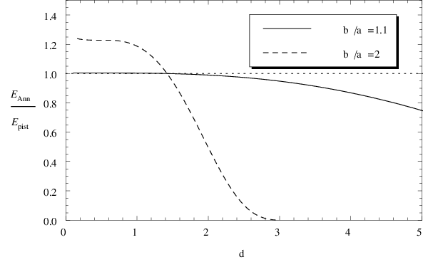
In Fig. 7 we define and the plateaus seen in the second figure may be understood from the proximity force approximation,
| (28) |
in comparison to the interaction between infinite parallel plates.
7 Applications of Multiple Scattering
As an illustration of practical calculations using the multiple scattering machinery, we illustrate in Fig. 8 a semi-infinite array of periodic potentials, such as a array of dielectric slabs, for which the exact Casimir-Polder force with an atom to the left may be calculated [14].
file=PeriodicPotential.eps,height=3cm
7.1 Casimir-Polder Force
Consider an atom, of polarizability , a distance to the left of the array. The Casimir-Polder energy is
| (29) |
where apart from an irrelevant constant the trace of the Green’s function is
| (30) |
Here the reflection coefficients are those for the entire array ( is the distance between the potential slabs),
| (31) |
If the potentials consist of dielectric slabs, with dielectric constant and thickness , the TE reflection and transmission coefficients for a single slab are ()
| (32a) | |||||
| (32b) | |||||
The TM reflection and transmission coefficients are obtained by replacing, except in the exponents, . (Multilayer potentials have been discussed extensively in the past, see, for example, Refs. [15, 16, 17, 18].)
For example, in the static limit, where we disregard the frequency dependence of the polarizability,
| (33) |
This is compared with the single slab result in Fig. 9.
t]

It is interesting to consider the limit, which is shown in Fig. 10.
file=Fig19.eps,height=4cm
When we recover the bulk limit. Such results apparently will have applications to experiment rather soon [19].
8 Exact Temperature Results
The scalar Casimir energy between two weak nonoverlapping potentials and at temperature is [20]
| (34) |
8.1 Exact Proximity Force Approximation
From Eq. (34) we find that the energy between a semitransparent plane and an arbitrarily curved nonintersecting semitransparent surface is for weak coupling
| (35) |
where the area integral is over the curved surface. Here is the distance between the plates at a given point on the surface . Equation (35) is precisely what one means by the proximity force approximation:
| (36) |
8.2 Interaction Between Semitransparent Spheres
We can, for weak scalar coupling, compute the energy between two spheres of radius and , whose centers are separated by a distance :
| (37) | |||||
where for is given by the power series,
| (38) |
which is obtained from the differential equation
| (39) |
Results for the energy obtained by solving this differential equation are shown in Fig. 11. For further details see Ref. [20].
[width=2.5in]plot2.eps
8.3 Mean distances between spheres
Encountered in the above calculation are mean powers of distances between spheres as defined by
| (40) |
for spheres, of radii and , respectively, separated by a center-to-center distance . Here and , and can in general be represented by the infinite series
| (41) |
Here the homogeneous polynomials are
| (42a) | |||||
| (42b) | |||||
| (42c) | |||||
| (42d) | |||||
Here in general,
| (43) |
There is also a recursion relation,
| (44) |
since is homogeneous in of degree .
For integer , is a polynomial of degree , and we can immediately find
| (45) | |||||
Although this was derived for integer it actually holds for all values of .
9 Conclusions
The multiple scattering formalism can be used to find numerical results effectively in many situations, as we have seen in this outline. Weak coupling results are exact and often given in closed form. The method can also be used to extract not only interaction energies but self energies, as described in Ref. [23].
Acknowledgements.
We thank the US National Science Foundation and the US Department of Energy for partial support of this research. We thank Elom Abalo, Nima Pourtolami, and K. V. Shajesh for collaborative assistance. We dedicate this paper to Emilio Elizalde.References
- (1) E. Komatsu et al., “Seven-Year Wilkinson Microwave Anisotropy Probe (WMAP) Observations: Cosmological Interpretation,” arXiv:1001.4538 [astro-ph.CO].
- (2) S. Weinberg, “The Cosmological Constant Problem,” Rev. Mod. Phys. 61, 1 (1989).
- (3) O. Kenneth and I. Klich, “Casimir Forces in a Operator Approach,” Phys. Rev. B 78, 014103 (2008) [arXiv:0707.4017 [quant-ph]].
- (4) J. Schwinger, L. L. DeRaad, Jr., K. A. Milton and W.-y. Tsai, Classical Electrodynamics, Advanced Book Program, Perseus Books (Westview Books) 1998.
- (5) J. S. Schwinger, L. L. DeRaad, Jr., and K. A. Milton, “Casimir Effect in Dielectrics,” Ann. Phys. (NY) 115, 1 (1979).
- (6) K. A. Milton, J. Wagner, P. Parashar and I. Brevik, “Casimir Energy, Dispersion, and the Lifshitz Formula,” Phys. Rev. D 81, 065007 (2010) [arXiv:1001.4163 [cond-mat.other]].
- (7) P. Parashar, K. A. Milton, I. Cavero-Peláez and K. V. Shajesh, “Electromagnetic Non-contact Gears: Prelude,” in K. A. Milton and M. Bordag, eds., Proceedings of the 9th Conference on Quantum Field Theory Under the Influence of External Conditions (World Scientific, Singapore, 2010), p. 48. arXiv:1001.4105 [cond-mat.other].
- (8) I. Cavero-Peláez, K. A. Milton, P. Parashar and K. V. Shajesh, “Non-Contact Gears: I. Next-to-Leading Order Contribution to Lateral Casimir Force Between Corrugated Parallel Plates,” Phys. Rev. D 78, 065018 (2008) [arXiv:0805.2776 [hep-th]].
- (9) T. Emig, A. Hanke, R. Golestanian and M. Kardar, “Normal and Lateral Casimir Forces Between Deformed Plates,” Phys. Rev. A 67, 022114 (2003).
- (10) I. Brevik, S. Å. Ellingsen and K. A. Milton, “Electrodynamic Casimir Effect in a Medium-Filled Wedge,” Phys. Rev. E 79, 041120 (2009) [arXiv:0901.4214 [quant-ph]].
- (11) S. Å. Ellingsen, I. Brevik and K. A. Milton, “Electrodynamic Casimir Effect in a Medium-Filled Wedge II,” Phys. Rev. E 80, 021125 (2009) [arXiv:0905.2088 [hep-th]].
- (12) S. Å. Ellingsen, I. Brevik and K. A. Milton, “Casimir Effect at Nonzero Temperature for Wedges and Cylinders,” Phys. Rev. D 81, 065031 (2010) [arXiv:1001.2630 [hep-th]].
- (13) K. A. Milton, J. Wagner and K. Kirsten, “Casimir Effect for a Semitransparent Wedge and an Annular Piston,” Phys. Rev. D 80, 125028 (2009) [arXiv:0911.1123 [hep-th]].
- (14) K. A. Milton, P. Parashar, J. Wagner, and I. Cavero-Peláez. “Multiple Scattering Casimir Force Calculations: Layered and Corrugated Materials, Wedges, and Casimir-Polder Forces,” arXiv:0910.3215 [hep-th], in the Proceedings of Casimir 2009, Yale, August 2009, J. Vac. Sci. Technol. B 28, C4A8-C4A16 (2010).
- (15) F. Zhou and L. Spruch, “Van der Waals and Retardation (Casimir) Interactions of an Electron or an Atom with Multilayered Walls,” Phys. Rev. A 52, 297 (1995).
- (16) M. S. Tomaš, “Casimir Force in Absorbing Multilayers,” Phys. Rev. A 66, 052103 (2002) [arXiv:quant-ph/0207106].
- (17) M. Bordag, G. Klimchitskaya, U. Mohideen, and V. M. Mostepanenko, Advances in the Casimir Effect (Oxford University Press, 2009).
- (18) V. A. Parsegian, Van der Waals Forces: A Handbook for Biologists, Chemists, Engineers, and Physicists (Cambridge University Press, 2006).
- (19) R. Salem, Y. Japha, J. Chabé, B. Hadad, M. Keil, K. A. Milton, and R. Folman, “Nanowire Atomchip Traps for Sub-Micron Atom-Surface Distances,” New J. Phys. 12, 023039, (2010).
- (20) K. A. Milton, P. Parashar, J. Wagner, and K.V. Shajesh, “Exact Casimir Energies at Nonzero Temperature: Validity of Proximity Force Approximation and Interaction of Semitransparent Spheres,” arXiv:0909.0977, to appear in Erber Festschrift, ed. P. Johnson.
- (21) R. S. Decca, E. Fischbach, G. L. Klimchitskaya, D. E. Krause, D. Lopez and V. M. Mostepanenko, “Application of the Proximity Force Approximation to Gravitational and Yukawa-Type Forces,” Phys. Rev. D 79, 124021 (2009) [arXiv:0903.1299 [quant-ph]].
- (22) D. A. R. Dalvit and R. Onofrio, “On the Use of the Proximity Force Approximation for Deriving Limits to Short-Range Gravitational-Like Interactions from Sphere-Plane Casimir Force Experiments,” Phys. Rev. D 80, 064025 (2009) [arXiv:0909.3068 [quant-ph]].
- (23) K. A. Milton, “Local and Global Casimir Energies: Divergences, Renormalization, and the Coupling to Gravity,” arXiv:1005.0031 [hep-th], to be published in a Lecture Notes in Physics volume by Springer.