2011 Vol. 11 No. XX, 000–000
Multiwavelength study of low-luminosity 6.7-GHz methanol masers ∗ 00footnotetext: Supported by the National Natural Science Foundation of China.
Abstract
We present results of 13CO(1–0), C18O(1–0), and HCO+(1–0) map observations and N2H+(1–0) single point observations directed towards a sample of nine low-luminosity 6.7-GHz masers. N2H+ line emission has been detected from six out of nine sources, C18O line emission has been detected from eight out of nine sources, and HCO+ and 13CO emission has been detected in all sources. In particular, a “blue profile” of the HCO+ spectrum, a signature of inflow, is found towards one source. From integrated intensity emission maps, we identified 17 cores in the sample. Among them, nine cores are closely associated with low-luminosity methanol masers. For these cores, we derive the column densities, core sizes, masses and molecular abundances. Comparison of our results with similar molecular line surveys towards the southern sky methanol masers indicates that linewidths of our sample, including only the low-luminosity masers, are smaller than the sample that includes both low- and high-luminosity masers. For the maser associated cores, their gas masses have the same order of magnitude as their virial masses, indicating that these cores are gravitationally bound systems. In addition, we have found from our observations that the low-luminosity methanol masers tend to coexist with H2O masers and outflows rather than with OH masers.
keywords
masers — ISM: abundances — ISM: molecules — stars: formation1 Introduction
Interstellar masers, such as the main-line hydroxy (OH) masers, 22-GHz water (H2O) masers and Class II methanol (CH3OH) masers, are one of the most readily observed signposts of star formation. These interstellar masers are powerful not only for signaling star formation regions, but also for diagnosing physical conditions (??), probing the kinematics of these regions (??) and measuring trigonometric parallaxes (??). Recently, with the advances of our understanding of these interstellar masers, ? even recommended using them to trace different evolutionary phases of massive star formation, which may shed light on our understanding of early evolutionary stages of massive stars.
Among these species, Class II methanol masers have some advantages over H2O and OH masers since they exclusively trace massive star-forming regions (??), while H2O and OH are known to also be associated with low mass star formation and evolved stars. To date, extensive surveys have yielded more than 800 6.7-GHz maser sites (???????). Recently, ? found distinctions between radio-quiet and radio-loud subgroups of 6.7-GHz methanol masers. ?, hereafter Paper I found remarkable physical and kinematic distinctions between faint and bright subgroups of 6.7-GHz masers. Hence, there is the potential to use elaborate classifications of 6.7-GHz masers based on their associations, e.g., UCH II regions, and inherent attributes. Such applications include using maser luminosities as a clock to indicate the evolutionary stage of ongoing massive star development.
Observationally, molecular emission is a powerful tool for investigating the physical and chemical conditions in hot cores. Transitions requiring different temperatures and densities for excitation constitute an excellent probe of physical conditions. It is known that 12CO is the most useful molecule tracer. When the 12CO(1–0) lines are optically thick in most opaque regions of molecular clouds, rarer CO isotopes, i.e., 13CO and C18O, are usually used instead to trace the cloud’s mass. In addition, HCO+ and N2H+ are important ionic molecules. Determining the abundance of HCO+ can reflect the ionization rate of clouds. Saturated and self absorbed line profiles of HCO+ are also used to trace dynamics, like the outflow and inflow of young protostellar objects (????). In contrast, N2H+ is an excellent tracer of quiescent high density gas (?). Moreover, since the chemical properties of hot cores vary with time, the relative molecular abundances can also be used as indicators of evolution (??). In this paper, we report our 3-mm spectral line observations, including 13CO(1–0), C18O(1–0), HCO+(1–0) and N2H+(1–0) transitions, towards a sample of nine faint 6.7-GHz methanol masers (Table 1). All nine sources have also been mapped in transitions of NH3(1,1), (2,2), (3,3) and 12CO(1–0) in Paper I. In Section 2, we describe the sample and observations. In Section 3, we present the results which include molecular line maps and individual descriptions. Analysis is given in Section 4. Finally, conclusions are drawn in Section 5.
| Source | RA (J2000) | Dec (J2000) | D | Other | Ref. | |||
|---|---|---|---|---|---|---|---|---|
| Name | (h m s) | (∘ ′ ′′) | (Jy) | (km s-1) | (kpc) | () | Name | |
| (1) | (2) | (3) | (4) | (5) | (6) | (7) | (8) | (9) |
| 106.80+5.31 | 22:19:18.3 | +63:18:48 | 0.5 | –2.0 | 0.94 | 7.0E–10 | S 140 | 13 |
| 111.25–0.77 | 23:16:09.7 | +59:55:29 | 4.0 | –38.5 | 3.58 | 8.5E–08 | IRAS 23139+5939 | 12 |
| 121.24–0.34 | 00:36:47.358 | +63:29:02.18 | 10 | –22.8 | 0.8515 | 1.3E–08 | L 1287 | 9,14 |
| 133.72+1.22 | 02:25:41.9 | +62:06:05 | 5 | –44.5 | 2.35 | 4.6E–08 | W3 IRS5 | 11 |
| 183.35–0.59 | 05:51:10.8 | +25:46:14 | 19 | –4.5 | 2.16 | 1.5E–07 | IRAS 05480+2545 | 11 |
| 188.80+1.03 | 06:09:07.8 | +21:50:39 | 4.8 | –5.5 | 21 | 3.3E–08 | AFGL 5182 | 12 |
| 189.03+0.78 | 06:08:40.671 | +21:31:06.89 | 17 | 8.8 | 1.57 | 6.6E–08 | AFGL 6466 | 2,14 |
| 189.78+0.34 | 06:08:35.28 | +20:39:06.7 | 15 | 5.7 | 1.5⋆ | 5.8E–08 | S 252A | 2,3 |
| 206.54–16.36 | 05:41:44.15 | –01:54:44.9 | 1.48 | 12.4 | 0.415 | 4.4E–10 | NGC 2024 | 10 |
Col. (1) is the source name which is named after Galactic coordinates, Cols. (2) and (3) are equatorial coordinates. Peak flux density, central velocity, distance and maser luminosity are listed in Cols. (4)(7), respectively. Other names and references are listed in Cols. (8) and (9), respectively.
References for sources and distances:
[1] ?; [2] ?; [3] ?; [4] ?; [5] ?; [6] ?; [7] ?; [8] ?; [9] ?; [10] ?; [11]?; [12]?; [13] ?; [14] ?; [15] ?;
⋆ Heliocentric kinematic distance.
2 Sample and Observations
2.1 Sample
The low-luminosity 6.7-GHz methanol masers in this study were mostly selected (seven out of nine) from the catalog of ? according to their lowest luminosities (the luminosities are calculated from the peak flux density assuming a typical linewidth of 0.25 km s-1 and isotropic emission). Two other sources with very low luminosities, 106.80+5.31 and 206.54–16.36, were selected from ? and ? respectively. The 6.7-GHz line luminosities of these sources range from 4.4 to 1.5 . Their properties, including galactic and equatorial coordinates, peak flux densities, central velocities, distances, luminosities, possible other names and references, are listed in Table 1. All of the sources have already been mapped in transitions of NH3(1,1), (2,2), (3,3) and 12CO() in Paper I.
2.2 Observations
The observations were performed during 2008 January and 2010 March with the 13.7-m millimeter wave telescope in Delingha, China. We mapped the nine sources in transitions of 13CO(1–0), C18O(1–0) and HCO+(1–0). A transition of N2H+(1–0) was observed with a single pointing, targeted at the maser sites. A cooled SIS receiver was employed (?), and system temperatures were 200 300 K during the observations. The Acousto-Optical Spectrometer (AOS) was used to measure the transitions of 13CO(1–0) and C18O(1–0) and the Fast Fourier Transform Spectrometer (FFTS) was used to measure the transitions of HCO+(1–0) and N2H+(1–0). The HPBW was 60′′ at 110 GHz. The observations were performed in a position switched mode. The grid spacing of the mapping observations was 30′′, and the average integration time was 5 min per point. The pointing accuracy was better than 10′′. Data were calibrated using the standard chopper wheel method. S140 and NGC 2264 were used for flux calibration and observed every two hours during the observations. Absolute calibration is estimated to be accurate to about 15%. Basic information of the observations is summarized in Table 2.
| Translation | HPBW | Bandwidth | 1 rsma | ||
|---|---|---|---|---|---|
| (GHz) | (′′) | (MHz) | (km s-1) | (K) | |
| 13CO(1–0) | 110.201353 | 60 | 43 | 0.11 | 0.10 |
| C18O(1–0) | 109.782182 | 60 | 43 | 0.12 | 0.10 |
| HCO+(1–0) | 89.188521 | 74 | 200 | 0.20 | 0.10 |
| N2H+(1–0) | 93.171880 | 71 | 1000 | 0.04 | 0.10 |
Notes: a typical value in the scale of brightness temperature for the reduced spectra.
Data were processed using the CLASS and GREG packages of GILDAS11 1 CLASS and GREG are part of the Grenoble Image and Line Data Analysis Software (GILDAS) working group’s software. http://www.iram.fr/IRAMFR/GILDAS/ software, including baseline subtraction, fitting Gaussian line profiles and hyperfine structure fitting (HFS) of N2H+(1–0) lines.
3 Results
N2H+ emission is detected in six sources, C18O emission is detected in eight sources, and 13CO and HCO+ are detected in all sources. Detected spectral lines are at least 3- above the baseline and in most cases have a signal to noise ratio greater than five. The detailed detections for individual sources are presented in Table 3. Recently, similar 3-mm spectral line surveys towards southern 6.7-GHz methanol masers presented high detection rates (99%) of HCO+(1–0), N2H+(1–0) and 13CO(1–0) (?). Our detection rates of 13CO(1–0) and HCO+(1–0) are 100%, similar to the 99% detection rates of ?, while our detection rate of N2H+(1–0) is 66%, lower than the 99% rate of ?. The lower detection rate of N2H+(1–0) may be due to the relatively lower sensitivity of our observations.
| Source Name | 13CO(1–0) | C18O(1–0) | HCO+(1–0) | N2H+(1–0) |
|---|---|---|---|---|
| 106.80+5.31 | Y | Y | Y | Y |
| 111.25–0.77 | Y | Y | Y | N |
| 121.24–0.34 | Y | Y | Y | Y |
| 133.72+1.22 | Y | N | Y | N |
| 183.35–0.59 | Y | Y | Y | Y |
| 188.80+1.03 | Y | Y | Y | N |
| 189.03+0.78 | Y | Y | Y | Y |
| 189.78+0.34 | Y | Y | Y | Y |
| 206.54–16.3 | Y | Y | Y | Y |
| Detection Rate | 9/9 | 8/9 | 9/9 | 6/9 |
Notes: “Y” indicates detection, “N” indicates no detection.
3.1 Spectra
In Figure 1, we present the 13CO(1–0), C18O(1–0), HCO+(1–0) and N2H+(1–0) spectra at the positions of the peak of the maser associated cores. 13CO(1–0), C18O(1–0), and HCO+(1–0) lines are fitted with Gaussian profiles. For HCO+(1–0) spectra with evidence of self absorbtion, though exhibiting a double-peak profile, are fitted with a single Gaussian function. Spectral parameters, i.e., bright temperatures, line width, velocity of the local standard of rest (), and integral intensities of 13CO(1–0), C18O(1–0), and HCO+(1–0), are listed in Table 4. For N2H+(1–0), following ?, we fit the spectra with two methods: (1) the hyperfine structure fitting routine in the CLASS software, considering the seven-component structure; (2) three-Gaussian fitting of the three blended groups. The fitted parameters of both methods are presented in Table 5.


 \vs
\vs


 \vs\vs


 \vs\vs


 \vs\vs


 \vs
\vs


 \vs
\vs


 \vs\vs


3.2 Maps
Contours of 13CO(1–0), C18O(1–0) and HCO+(1–0) integrated intensities are presented in Figure 2. We use infrared dust emission, from the Midcourse Space Experiment (MSX) E band (21 m) images, as the background for the contours. For 106.80+5.31, where no MSX data are available, the Multiband Imaging Photometer for Spitzer (MIPS) 24 m image is used. The central blank pixels in the 24 m image are due to saturation. The squares, triangles, pluses and ellipses in Figure 2 denote the 6.7-GHz CH3OH masers, H2O masers, OH masers and error ellipses of the IRAS point sources in the fields, respectively. We use C18O(1–0) (optical thin line) contours to define a concentrated structure, i.e., a core, and determine the size and position of the core. Although for 133.72+1.22 where there is no detection of C18O, the cores are identified from the 13CO map and core 1 of 189.78+0.34, where there is no C18O emission peak, is identified from the HCO+ map. Cores were identified using visual inspection. The methodology used to define cores is similar to the operation of the “CLUMPFIND” algorithm (?). Totally, we find 17 cores from the nine fields, with eight cores showing no maser associations.
| 13CO | C18O | HCO+ | |||||||||||||||
|---|---|---|---|---|---|---|---|---|---|---|---|---|---|---|---|---|---|
| Region | Coreα | ||||||||||||||||
| (K) | (K km s-1) | (km s-1) | ( km s-1) | (K) | (K km s-1) | (km s-1) | (km s-1) | (K) | (K km s-1) | ( km s-1) | ( km s-1) | ||||||
| 106.80+5.31 | 1 | 12.22 | 42.34 | –7.46(01) | 3.26(02) | 1.85 | 5.73 | –7.52(04) | 2.91(11) | 17.82 | 53.71 | –6.74(01) | 2.83(02) | ||||
| 111.25–0.77 | 1 | 9.78 | 27.43 | –44.09(01) | 2.64(03) | 1.14 | 2.49 | –44.28(04) | 2.05(11) | 1.37 | 4.79 | –44.02(05) | 3.27(14) | ||||
| 121.24–0.34 | 1 | 9.06 | 21.46 | –17.39(01) | 2.22(03) | 1.57 | 3.11 | –17.15(04) | 1.87(08) | 8.70 | 27.75 | –17.53(02) | 3.00(06) | ||||
| 133.72+1.22 | 1 | 8.35 | 29.18 | — | — | — | — | — | — | 1.81 | 9.52 | –40.57(05) | 4.91(14) | ||||
| 133.72+1.22 | 2 | 5.67 | 29.75 | –43.37(01) | 4.93(03) | — | — | — | — | 1.41 | 7.39 | –41.89(05) | 4.91(14) | ||||
| 133.72+1.22 | 3 | 8.17 | 46.05 | –38.88(03) | 5.40(02) | — | — | — | — | 1.40 | 7.00 | –36.14(05) | 4.71(14) | ||||
| 133.72+1.22 | 4 | 9.06 | 28.15 | –38.88(02) | 2.92(02) | — | — | — | — | 1.38 | 4.14 | –39.50(05) | 2.81(15) | ||||
| 183.35–0.59 | 1 | 7.30 | 18.44 | –9.25(01) | 2.37(02) | 1.16 | 2.34 | –9.24(04) | 1.90(10) | 4.25 | 12.17 | –9.76(05) | 2.69(15) | ||||
| 188.80+1.03 | 1 | 6.99 | 20.63 | –0.58(01) | 2.77(02) | 1.00 | 2.83 | –0.39(06) | 2.65(15) | 0.68 | 1.81 | –1.25(06) | 2.54(16) | ||||
| 188.80+1.03 | 2 | 6.96 | 21.90 | –0.17(01) | 2.96(02) | 1.35 | 2.97 | –0.41(02) | 2.08(05) | 0.66 | 1.99 | –1.15(07) | 2.83(16) | ||||
| 189.03+0.78 | 1 | 8.31 | 26.70 | 2.79(01) | 3.02(02) | 1.26 | 3.66 | 2.81(06) | 2.74(13) | 5.44 | 18.47 | 2.59(01) | 3.19(04) | ||||
| 189.03+0.78 | 2 | 8.56 | 24.27 | 2.32(01) | 2.66(03) | 1.63 | 3.82 | 2.13(03) | 2.20(09) | 3.06 | 10.19 | 2.28(35) | 3.12(09) | ||||
| 189.78+0.34 | 1 | 12.26 | 41.28 | 8.64(01) | 3.16(02) | 2.21 | 4.81 | 8.55(02) | 2.24(05) | 2.77 | 13.52 | 7.99(04) | 4.58(09) | ||||
| 189.78+0.34 | 2 | 11.89 | 49.23 | 8.15(01) | 3.89(01) | 2.39 | 7.18 | 8.04(02) | 3.03(05) | 2.05 | 8.32 | 7.70(05) | 3.83(13) | ||||
| 189.78+0.34 | 3 | 10.92 | 45.76 | 8.31(01) | 3.94(01) | 2.68 | 5.09 | 7.67(02) | 1.96(07) | 1.39 | 5.83 | 7.78(08) | 3.94(19) | ||||
| 206.54–16.36 | 1 | 20.43 | 57.08 | 10.33(01) | 2.68(01) | 3.81 | 7.49 | 10.04(02) | 1.94(06) | 3.47 | 10.97 | 10.06(03) | 2.66(09) | ||||
| 206.54–16.36 | 2 | 21.27 | 66.54 | 10.61(01) | 2.94(02) | 3.17 | 9.48 | 10.28(02) | 2.81(04) | 4.45 | 17.54 | 10.72(04) | 3.70(07) | ||||
Notes: : 1, 2, 3, and 4 denote the different components in the same field.


 \vs
\vs


 \vs
\vs


 \vs\vs


3.3 Comments on Individual Sources
- –
106.80+5.31 — This source is located in the central part of the S140 molecular complex. Both the 13CO(1–0) and C18O(1–0) maps show a filamented structure extending southwest to northeast and peak at the central infrared source. The HCO+ map reveals a single core surrounding the central infrared source. All the three maser species, i.e., CH3OH, H2O and OH masers, were found in this region.
- –
111.25–0.77 — There is a single core peak towards the IRAS 23139+5939. The 13CO maps reveal an extended emission elongating towards the northern direction. Both H2O and CH3OH masers were found in this region.
- –
121.24–0.34 — There is a single core which elongates northwest to southeast and peaks at IRAS 00338+6312. Both H2O and CH3OH masers were found in this region.
- –
133.72+1.22 — This is an intensively studied region of active star formation, the W3 complex. 13CO(1–0) and HCO+(1–0) spectra show two velocity components, with velocity ranges of km s-1 and km s-1, respectively. In the 13CO integrated intensity map with a velocity range of –48–42 km s-1, one can see a two-core structure, with the eastern core (Core 1) peaking towards the CH3OH maser and the western core (Core 2) associated with the western mid-infrared dust core. In the 13CO integrated intensity map with a velocity range of –40–36 km s-1, there is a filament consisting of two cores, with the northwestern core (Core 3) departing 30′′ south of IRAS 02219+6152 and the southeastern core (Core 4) departing 2′ southeast of the IRAS source. Emission of HCO+ shows a similar distribution. Three H2O and one CH3OH masers are found in this field.
- –
183.35–0.59 — A single core is located southwest and with an offset of 15′′ from IRAS 05480+2545. Only the CH3OH maser is found in this region.
- –
188.80+1.03 — Both C18O(1–0) and HCO+ maps reveal a filament consisting of two cores which extend southwest to northeast through the field. Core 1 (the southeast core) is offset by 30′′ southeast towards IRAS source 06061+2151 and Core 2 (the northwest core) is offset by 30′′ northeast towards the IRAS source. H2O and CH3OH masers are found in this region.
- –
189.03+0.78 — The mid-infrared dust emission of this region shows two heat sources. Emission of CO and HCO+ reveals a filament extending from the southwest infrared source towards the northeast one. The filament in the C18O map consists of two cores. The southwestern core (Core 1) is associated with IRAS 06056+2131. The northeastern core (Core 2) is located in the middle of the two mid-infrared cores departing 1′ northeast towards IRAS 06056+2131. Both H2O and CH3OH masers are found to be associated with Core 1.
- –
189.78+0.34 — This source is part of the S252A molecular complex. 13CO and C18O maps reveal a filamented structure consisting of two cores and extending from north to south, while the HCO+ map presents a filament extending northwest to southeast and peaking towards the CH3OH maser.
- –
206.54–16.36 —It is located in the vicinity of the NGC 2024 HII region. A filament, called the “Molecular Ridge,” is elongated in the north-south direction (?). The filament is segregated into two segments on the C18O maps. Along the ridge, there are seven far infrared sources (??). The CH3OH maser is associated with FIR4 (?).
| 7-component HFS fits α | 3-Gaussian fits γ | ||||||||||
| Group-1 | Group-2 | Group-3 | |||||||||
| Source | |||||||||||
| (km s-1) | (km s-1) | (K km s-1) | (km s-1) | (K km s-1) | (km s-1) | (K km s-1) | (km s-1) | ||||
| 106.80+5.31 | –6.95(02) | 1.71(05) | 1.20 | 2.15(19) | 4.82 | 2.48(20) | 2.87 | 2.41(39) | |||
| 121.24–0.34 | –17.75(03) | 1.56(07) | 0.43 | 1.84(24) | 1.99 | 2.39(19) | 1.02 | 1.96(24) | |||
| 183.35–0.59 | –9.70(06) | 1.60(11) | 0.26 | 1.41(30) | 1.24 | 2.39(20) | 0.70 | 2.11(34) | |||
| 189.03+0.78 | 2.58(06) | 1.85(13) | 0.40 | 2.01(46) | 1.79 | 2.50(30) | 1.27 | 3.14(17) | |||
| 189.78+0.34 | 7.44(06) | 1.55(15) | 0.23 | 0.94(34) | 1.43 | 2.47(28) | 1.22 | 2.93(74) | |||
| 206.54-16.36 | 10.62(06) | 1.30(12) | — | — | 1.07 | 2.09(25) | 0.63 | 1.82(23) | |||
Notes: : fitted with the CLASS HFS routine considering the 7-component structure;
: is referring to the transition, i.e. the center component of ‘Group-2’;
: Gaussian fits to the three groups.
3.4 Physical Quantities
3.4.1 Optical depth and excitation temperature
In this section, we derive optical depths and excitation temperatures of CO and N2H+ transitions. For 13CO and C18O, the optical depths and excitation temperatures are estimated by assuming 12CO(1–0) lines are optically thick with formulae 1–3 of ?. For N2H+, due to the uncertainty introduced by the blended profiles, optical depths of N2H+ cannot be directly fitted with the HFS routine, but rather can be derived from the ratio of integrated intensities, , of the three blended groups with a method of ?, using equation
| (1) |
where ‘a’ is the expected ratio of , which should be 1: 5: 2 under optically thin conditions. It is noted that the optical depth derived here is the “group optical depth” that contains contributions of (2112), (2312) and (2211) components.
Then we derived (2312) excitation temperatures of N2H+(1–0) using equation
| (2) |
where and are brightness temperature and optical depth for the (2312) component, , and K.
The optical depths and excitation temperatures of 13CO, C18O and N2H+ are tabulated in Table 6. The typical optical depths are 0.7, 0.08 and 0.3 for 13CO, C18O and N2H+, respectively. CO excitation temperatures range from 15 K to 48 K, with a mean value of 28 K. Excitation temperatures for N2H+ range from 5 K to 12 K, with a mean value of 7 K. Since the calculations are based on a uniform beam filling factor, the excitation temperatures (especially for N2H+) derived here should be the lower limits of the true values.
| Optical Depth | Excitation Temperature | Column Density | Abundance γ | ||||||||||||||
| Region | Core | 13CO | C18O | N2H+ α | (CO) | (N2H+)β | 13CO | C18O | N2H+ | X(C18O) | X(N2H+) | ||||||
| (K) | (K) | (cm-2) | (cm-2) | cm-2 | |||||||||||||
| 106.80+5.31 | 1 | 0.62 | 0.08 | 0.30 | 32.8(4.9) | 12.1(2.9) | 9.50E+16 | 1.01E+16 | 8.96 | 2.12 | 1.89E–10 | ||||||
| 111.25–0.77 | 1 | 0.85 | 0.07 | — | 23.8(3.6) | — | 5.09E+16 | 3.26E+15 | — | 1.28 | — | ||||||
| 121.24–0.34 | 1 | 0.80 | 0.10 | 0.27 | 22.0(3.3) | 7.4(2.7) | 3.63E+16 | 3.85E+15 | 2.48 | 2.12 | 1.37E–10 | ||||||
| 133.72+1.22 | 1 | 0.31 | — | — | 35.0(5.7) | — | 6.01E+16 | — | — | — | — | ||||||
| 133.72+1.22 | 2 | 0.24 | — | — | 38.3(5.7) | — | 6.46E+16 | — | — | — | — | ||||||
| 133.72+1.22 | 3 | 0.33 | — | — | 32.3(4.8) | — | 8.60E+16 | — | — | — | — | ||||||
| 133.72+1.22 | 4 | 0.49 | — | — | 27.7(4.5) | — | 5.14E+16 | — | — | — | — | ||||||
| 183.35–0.59 | 1 | 1.02 | 0.13 | 0.32 | 21.2(3.2) | 5.1(3.1) | 3.32E+16 | 2.85E+15 | 1.23 | 1.72 | 7.42E-11 | ||||||
| 188.80+1.03 | 1 | 0.69 | 0.07 | — | 20.7(3.1) | — | 3.15E+16 | 3.27E+15 | — | 2.08 | — | ||||||
| 188.80+1.03 | 2 | 1.23 | 0.17 | — | 14.6(2.2) | — | 3.12E+16 | 2.68E+15 | — | 1.72 | — | ||||||
| 189.03+0.78 | 1 | 0.72 | 0.08 | 0.25 | 23.1(3.5) | 7.3(6.3) | 4.56E+16 | 4.69E+15 | 2.19 | 2.06 | 9.62E–11 | ||||||
| 189.03+0.78 | 2 | 0.89 | 0.14 | — | 17.2(2.6) | — | 3.45E+16 | 3.89E+15 | — | 2.26 | — | ||||||
| 189.78+0.34 | 1 | 0.72 | 0.09 | 0.37 | 33.1(4.9) | 5.0(2.3) | 9.76E+16 | 8.58E+15 | 1.44 | 1.76 | 2.94E–11 | ||||||
| 189.78+0.34 | 2 | 0.82 | 0.13 | — | 29.1(4.4) | — | 1.08E+17 | 1.16E+16 | — | 2.15 | — | ||||||
| 189.78+0.34 | 3 | 0.76 | 0.16 | — | 27.1(4.1) | — | 9.17E+16 | 7.82E+15 | — | 1.71 | — | ||||||
| 206.54–16.36 | 1 | 0.94 | 0.09 | 0.33 | 36.0(5.4) | 5.0(4.3) | 1.60E+17 | 1.44E+16 | 1.05 | 1.80 | 1.31E–11 | ||||||
| 206.54–16.36 | 2 | 1.54 | 0.13 | — | 36.7(5.5) | — | 2.42E+17 | 1.90E+16 | — | 1.57 | — | ||||||
| meanδ | — | 0.74 | 0.09 | 0.31 | 27.52 | 6.97 | 6.78E+16 | 6.37E+15 | 2.89 | 1.87 | 8.98E–11 | ||||||
| median | — | 0.72 | 0.09 | 0.31 | 23.80 | 6.20 | 5.09E+16 | 4.27E+15 | 1.83 | 1.93 | 8.52E–11 | ||||||
: (N) is the “group optical depth” that contains contributions of (2112), (2312) and (2211) components;
: is (2312) excitation temperature;
: the abundances were derived with the assumption of X(13CO) ;
: mean and median values are only for cores associated with masers, i.e., Core 1.
3.4.2 Column density and chemical abundance
With optical depths and excitation temperatures, total column densities of 13CO, C18O and N2H+ can be obtained from (eq. (A1), Scoville et al. 1986)
| (3) |
where is the rotational constant of the molecule and is the permanent dipole moment of the molecule. The values of and are taken to be 55.101 MHz and 0.1098 Debye for 13CO, 54.891 MHz and 0.1098 Debye for C18O (?), and 46.587 MHz and 3.37 Debye for N2H+ (?). is the rotational quantum number of the lower state in the observed transitions. Column densities of 13CO, C18O and N2H+ are presented in Table 6. Typical column densities of 13CO, C18O and N2H+ are 51016, 41015 and 11012 cm-2, respectively. For HCO+, whose excitation temperature and optical depth are lacking, we are unable to calculate reliable column densities. It is noted that the column densities, especially for N2H+, estimated here should be the lower limits, because of the underestimate of excitation temperatures. The total N2H+ column density calculated with an excitation temperature of 20 K should be three times larger than the value estimated with an excitation temperature of 5 K.
The relative abundance X between two species may be found directly from the ratio of their volume densities. Assuming both molecules occupy the same volume of space, the ratio of two species X= . Recently, the COMPLETE molecular survey gave an estimated value of [H2/13CO] in the range of 2.8 to 4.9 105 (?). The chemical evolution model suggested a more stable CO abundance relative to HCO+ and N2H+ (?). Thus, assuming a moderate 13CO abundance of 310-6, we derived the molecular abundances of C18O and N2H+ for the targeted low-luminosity 6.7-GHz maser regions. The results of column densities and chemical abundances are presented in Table 6.
The abundances of C18O range from 1.3 to 2.310-7, with a median value of 1.910-7, but the abundances of N2H+ range from 1.310-11 to 1.910-10, with a median value of 8.510-11. In contrast, the abundance fluctuation of N2H+ is more dramatic than that of C18O.
3.4.3 Core size and mass
The nominal core sizes, , were determined from contours of the C18O integral intensities by de-convolving the telescope beam, using Equation (4),
| (4) |
where is the distance, is the half-power angular size of the core, and is the half-power beam width of the telescope.
Core masses were computed by assuming a Gaussian column density distribution with a full-width at half-maximum (FWHM) of . If ) is the molecular hydrogen column density of the peak position, is the mass of a hydrogen molecule and is the ratio of total gas mass to hydrogen mass (assumed to be 1.36 based on ?), the core mass is given by
| (5) |
With linewidths and core sizes, we also estimated the virial masses following the approach by ?
| (6) |
where is the radius of the core in pc, is the FWHM linewidth of C18O in km s-1 and is the virial mass in .
The estimated nominal core sizes, gas masses and virial masses are tabulated in Table 7.
| Region | Core | R.A. | Dec. | Angular | Size | (H2) | ||
| Name | (h m s) | (∘ ′ ′′) | () | (pc) | ( cm-2) | () | () | |
| (1) | (2) | (3) | (4) | (5) | (6) | (7) | (8) | (9) |
| 106.80+5.31 | 1 | 22:19:20.0 | +63:19:10 | (120, 90) | 0.33 | 4.75 | 134 | 88 |
| 111.25–0.77 | 1 | 23:16:10.0 | +59:55:30 | (70, 60) | 0.37 | 2.55 | 91 | 49 |
| 121.24–0.34 | 1 | 00:36:47.8 | +63:28:57 | (110, 70) | 0.23 | 1.82 | 25 | 25 |
| 133.72+1.22 | 1 | 02:25:41.8 | +62:06:05 | (30, 30) | 0.29 | 3.01 | 66 | 220 |
| 133.72+1.22 | 2 | 02:25:32.0 | +62:06:22 | (120, 90) | 0.84 | 3.23 | 592 | 638 |
| 133.72+1.22 | 3 | 02:25:41.8 | +62:05:40 | (150, 90) | 0.98 | 4.30 | 1073 | 685 |
| 133.72+1.22 | 4 | 02:25:53.5 | +62:04:35 | (90, 60) | 0.42 | 2.57 | 118 | 105 |
| 183.35–0.59 | 1 | 05:51:10.5 | +25:46:05 | (120, 90) | 0.76 | 1.66 | 249 | 86 |
| 188.80+1.03 | 1 | 06:09:06.5 | +21:50:20 | (90, 70) | 0.45 | 1.58 | 83 | 100 |
| 188.80+1.03 | 2 | 06:09:09.4 | +21:51:06 | (75, 70) | 0.35 | 1.56 | 50 | 48 |
| 189.03+0.78 | 1 | 06:08:41.0 | +21:31:08 | (70, 70) | 0.23 | 2.28 | 31 | 54 |
| 189.03+0.78 | 2 | 06:08:44.5 | +21:31:40 | (90, 60) | 0.27 | 1.73 | 33 | 41 |
| 189.78+0.34 | 1 | 06:08:34.5 | +20:39:00 | (100, 80) | 0.43 | 4.88 | 235 | 68 |
| 189.78+0.34 | 2 | 06:08:40.5 | +20:38:00 | (90, 60) | 0.27 | 5.40 | 102 | 78 |
| 189.78+0.34 | 3 | 06:08:40.5 | +20:36:30 | (90, 60) | 0.27 | 4.59 | 87 | 33 |
| 206.54–16.36 | 1 | 05:41:43.5 | –01:54:05 | (90, 80) | 0.11 | 8.00 | 25 | 13 |
| 206.54–16.36 | 2 | 05:41:45.0 | –01:56:05 | (120, 100) | 0.16 | 12.10 | 81 | 40 |
| Mean | — | — | — | — | 0.36 | 3.39 | 104 | 78 |
| Median | — | — | — | — | 0.33 | 2.55 | 83 | 68 |
Cols. (3) and (4) are equatorial coordinates, Col. (5) is angular extensions of the major and minor axes of the core assuming a spherical geometry. Col. (6) is the nominal core size. Col. (7) is molecular hydrogen column density, (H2). Gas masses and virial masses are listed in Cols. (8)(9), respectively. Mean and median values of these quantities are listed in the last two rows.
4 Discussion
4.1 Line Profiles
Line profiles of 13CO and C18O are relatively simple and can be well fitted with a single Gaussian. In Figure 4 we present example spectra for the source 121.24–0.34 alongside the 13CO(1–0) contour. The spectrum of N2H+ is fitted with the HFS routine in the CLASS software to simultaneously fit the N2H+ profiles with seven Gaussian distributions. In case of a cold quiescent environment, e.g., a dark cloud, the spectrum of N2H+(1–0) can exhibit seven hyperfine components (?). In our case, however, the seven components of N2H+ are blended into three groups due to large linewidths.
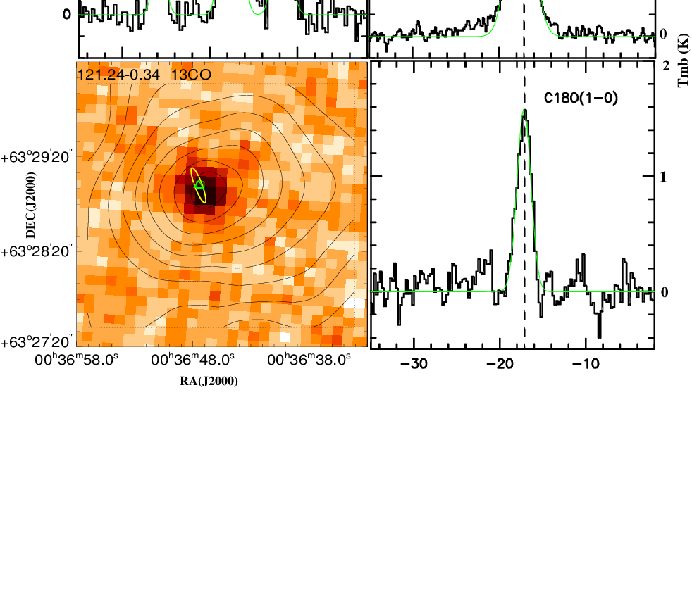

In Figure 4, the spectrum of HCO+ exhibits a double-peak profile. By contrast, the spectrum of C18O, an optically thin line, shows a single peak located at the dip of HCO+, which indicates that the double-peak profile of HCO+(1–0) is a self-absorption feature. Therefore, we fit the HCO+ spectrum with a single Gaussian by blanking the absorption dip. This “blue profile” is considered as a signature of inflow. ? conducted an HCO+ survey towards high mass star forming regions and obtained a high rate of incidence for this kind of “blue profile” (29%). However, in our sample, this inflow signature is only found towards 121.24–0.34, corresponding to a rate of 11%. In addition, the self-absorption feature is also found in the HCO+ spectrum of 206.54–16.36, but in contrast to 121.24–0.34, the HCO+ spectrum of 206.54–16.36 shows an excess of the red profile which may be evidence of expansion. ? established a sophisticated model based on the scenario of a PDR and the “Blister model” to interpret the complex line shapes of the multiple CO transition from 206.54–16.36.
Figure 4 shows the linewidth of the four molecules as an function of maser luminosity. The mean linewidths towards these low-luminosity maser regions are as follows: HCO+: 3.3 km s-1, 13CO: 2.8 km s-1, C18O: 2.3 km s-1 and N2H+: 1.6 km s-1. In general, linewidths of HCO+ are larger than 13CO, C18O and N2H+. ?? surveyed 83 southern methanol masers and obtained larger mean linewidths: HCO+: 5.1 km s-1, 13CO: 4.8 km s-1, and N2H+: 3.0 km s-1. It is obvious that linewidths in our sample, including only low-luminosity masers, are smaller than ??’s sample, which are composed of both high- and low-luminosity masers. Previous observations of ammonia also indicate that NH3(1,1) (2,2) linewidths of low-luminosity maser regions are smaller than those of high-luminosity maser regions (Paper I).
4.2 Gas Mass vs Virial Mass
In Figure 5 we plot the diagram of gas mass versus virial mass. For the maser associated cores, ranges from 25 to 250 , with a mean value of 104 and ranges from 13 to 220 , with a mean value of 78 . We can see that the value of and are consistent with having the same magnitude. As a general rule, clouds with are considered to be gravitationally bound systems. Generally, we propose that cores that contain low-luminosity 6.7-GHz methanol masers should be gravitationally bound.

4.3 Associations
Apart from Class II methanol masers, outflows, and bright IRAS sources, H2O and OH masers are also signatures of star formation. Since our targeted sources are all methanol masers, it is meaningful to investigate the associations of methanol masers with other star-forming phenomena, such as outflows, bright IRAS sources and two other kinds of masers. In Table 8, we list these associations. The association rates for the IRAS source, outflow and H2O are all 7/9, but the association rate for the OH maser is only 2/9. Positions of OH, H2O and IRAS sources are also marked in Figure 2 to show their spatial coexistence. We can see that these low-luminosity methanol masers are highly coincident with bright IRAS sources, outflows and H2O masers. In contrast, associations of OH masers are relatively weak. Though the number of studied cases in our sample is limited, our sample clearly indicates the fact that the Class II methanol maser phase is more likely to be overlaid on outflow and the H2O maser phrase than to be overlaid on the OH maser phrase (??).
| Source Name | IRAS Name | Outflow | H2O | OH |
|---|---|---|---|---|
| 106.80+5.31 | 22176+6303 | Y [1] | Y [5] | Y [7] |
| 111.25–0.77 | 23139+5939 | Y [1] | Y [5] | N [8] |
| 121.24–0.34 | 00338+6312 | Y [1] | Y [5] | … |
| 133.72+1.22 | 02219+6152 | Y [1] | Y [5] | N [7] |
| 183.35–0.59 | 05480+2545 | N [2] | N [5] | … |
| 188.80+1.03 | 06061+2151 | N [3] | Y [5] | N [7] |
| 189.03+0.78 | 06056+2131 | Y [1] | Y [5] | N [7] |
| 189.78+0.34 | N | Y [4] | Y [6] | … |
| 206.54–16.3 | N | Y [1] | N [5] | Y [9] |
| Association Rate | 7/9 | 7/9 | 7/9 | 2/9 |
Notes: “Y” indicates association, “N” indicates no association, “…” indicates that no information is available;
References — [1] ?; [2] ?; [3] ?; [4] ?; [5] ?; [6] ?; [7] ?; [8] ?; [9] ?.
\vs\vs5 Conclusions
We have performed multi-line observations, including transitions of 13CO(1–0), C18O(1–0), HCO+(1–0) and N2H+(1–0), towards nine low-luminosity 6.7-GHz methanol masers. From integrated intensity emission maps, we identified 17 cores, among which nine cores are closely associated with low-luminosity masers and eight cores lack maser associations. Physical quantities of these cores were derived, including column densities, core sizes, masses and molecular abundances. Our major findings are as follows:
- (1)
Linewidths of 13CO, HCO+ and N2H+ of these low-luminosity maser regions are smaller than ??’s sample.
- (2)
A “blue profile” of the HCO+(1–0) spectrum, signature of inflow, is found towards one source, the detection rate of which is three times less than ?.
- (3)
N2H+ abundances of these regions show larger fluctuations than those of CO.
- (4)
Virial masses and gas masses of the maser associated cores are consistent with having the same magnitude, indicating that these cores that contains low-luminosity 6.7-GHz masers are gravitationally bound systems.
- (5)
These low-luminosity masers are more inclined to coexist with H2O masers, outflows and bright IRAS sources rather than to coexist with OH masers.
We however caution that the number of sources in our study is limited. Consequently, the findings of this work have to be confirmed by a much larger sample.
Acknowledgements.
We wish to thank all the staff at Qinghai Station of Purple Mountain Observatory for their assistance with our observations. This work was supported by the National Natural Science Foundation of China (Grant Nos. 10673024, 10733030, 10703010 and 10621303) and the National Basic Research Program of China-973 Program (2007CB815403).Bibliography
- Baudry, A., Desmurs, J. F., Wilson, T. L., & Cohen, R. J. 1997, A&A, 325, 255
- Bergin, E. A., & Langer, W. D. 1997, ApJ, 486, 316
- Botschwina, P. 1984, Chem. Phys. Lett., 107, 535
- Breen, S. L., Ellingsen, S. P., Caswell, J. L., & Lewis, B. E. 2010, MNRAS, 401, 2219
- Carpenter, J. M., Snell, R. L., & Schloerb, F. P. 1995, ApJ, 445, 246
- Caswell, J. L., Vaile, R. A., Ellingsen, S. P., Whiteoak, J. B., & Norris, R. P. 1995, MNRAS, 272, 96
- Caswell, J. L. 2009, PASA, 26 , 454
- Chandler, C. J., & Carlstrom, J. E. 1996, ApJ, 466, 338
- Crampton, D., & Fisher, W. A. 1974, PDAO, 14, 283
- Ellingsen, S. P., Voronkov, M. A., Cragg, D. M., Sobolev, A. M., Breen, S. L., & Godfrey, P. D. 2007, IAUS, 242, 213
- Ellingsen, S. P. 2007, MNRAS, 377, 571
- Emprechtinger, M., Wiedner, M. C., Simon, R., et al. 2009, A&A, 496, 731
- Fuller, G. A., Williams, S. J., & Sridharan, T. K. 2005, A&A, 442, 949
- Georgelin, Y. M., & Georgelin, Y. P. 1976, A&A, 49, 57
- Green, J. A., Caswell, J. L., Fuller, G. A., et al. 2009, MNRAS, 392, 783
- Hildebrand, R. H. 1983, QJRAS, 24, 267
- Hughes, V. A., & MacLeod, G. C. 1993 AJ, 105, 1495
- Humphreys, R. M. 1978, ApJS, 38, 309
- Kim, K. T., & Kurtz, S. E. 2006, ApJ, 643, 978
- Klaassen, P. D., & Wilson, C. D. 2007, ApJ, 663, 1092
- Knowles, S. H., Caswell, J. L., & Goss, W. M. 1976, MNRAS, 175, 537
- Lada, C. J., Blitz, L., Reid, M. J., & Moran, J. M. 1981, ApJ, 243, 769
- Langer, W. D., van Dishoeck, E. F., Bergin, E. A., Blake, G. A., Tielens, A. G. G. M., Velusamy, T., & Whittet, D. C. B. 2000, in Protostars and Planets IV (Tucson: Univ. Arizona Press), 29
- Larionov, G. M., Val’tts, I. E., Winnberg, A., Johansson, L. E. B., Booth, R. S., & Golubev, V. V. 1999, A&AS, 139, 257
- Lovas, F. J., & Krupenie, P. H. 1974, J. Phys. Chem. Ref. Data, 3, 245
- MacLeod, G. C., van der Walt, D. J., North, A., Gaylard, M. J., Galt, J. A., & Moriarty-Schieven, G. H. 1998 AJ, 116, 2936
- MacLaren, I., Richardson, K. M., & Wolfendale, A. W. 1988, ApJ, 333, 821
- Mezger, P. G., Chini, R., Kreysa, E., Wink, J. E., & Salter, C. J. 1988, A&A, 191, 44
- Mezger, P. G., Sievers, A. W., Haslam, C. G. T., Kreysa, E., Lemke, R., Mauersberger, R., & Wilson, T. L. 1992, A&A, 256, 631
- Motogi, K., Watanabe, Y., Sorai, K., et al. 2008, MNRAS, 390, 532
- Minier, V., Ellingsen, S. P., Norris, R. P., & Booth, R. S. 2003, A&A, 403,1095
- Pandian, J. D., Goldsmith, P. F., & Deshpande, A. A. 2007, ApJ, 656, 255
- Pavlakis, K. G., & Kylafis, N. D. 1996a, ApJ, 467, 300
- Pavlakis, K. G., & Kylafis, N. D. 1996b, ApJ, 467, 309
- Pestalozzi, M. R., Minier, V., & Booth, R. S. 2005, A&A, 432, 737
- Pineda, J. E., Caselli, P., & Goodman, A. A. 2008 ApJ, 679, 481
- Purcell, C. R., Balasubramanyam, R., Burton, M. G., et al. 2006, MNRAS, 367, 553
- Purcell, C. R., Longmore, S. N., Burton, M. G., Walsh, A. J., Minier, V., Cunningham, M. R., & Balasubramanyam, R. 2009, MNRAS, 394, 323
- Reid, M. J., Menten, K. M., Zheng, X. W., et al. 2009, ApJ, 700, 137
- Scoville, N. Z., Sargent, A. I., Sanders, D. B., Claussen, M. J., Masson, C. R., Lo, K. Y., & Phillips, T. G. 1986, ApJ, 303, 416
- Slysh, V. I., Val’tts, I. E., Kalenskii, S. V., Voronkov, M. A., Palagi, F., Tofani, G., & Catarzi, M. 1999, A&AS, 134, 115
- Snell, R. L., Dickman, R. L., & Huang, Y. L. 1990, ApJ, 352, 139
- Szymczak, M., Hrynek, G., & Kus, A. J. 2000, A&AS, 143, 269
- Szymczak, M., & Kus, A. J. 2000, A&AS, 147, 181
- Sun, Y. & Gao, Y. 2009, MNRAS, 392, 170
- Torrelles, J.M., Patel, N., Gómez, J. F., Anglada, G., & Uscanga, L. 2005, Ap&SS 295, 53
- Valdettaro, R., Palla, F., Brand, J., et al. 2001, A&A, 368, 845
- Williams, J. P., de Geus, E. J. & Blitz, L. 1994, ApJ, 428, 693
- Womack, M., Ziurys, L. M., & Wyckoff, S. 1992, ApJ, 387, 417
- Wu, Y., Wei, Y., Zhao, M., Shi, Y., Yu, W., Qin, S., & Huang, M. 2004, A&A, 426, 503
- Wu, Y. F., Henkel, C., Xue, R., Guan, X., & Miller, M. 2007, ApJ, 669, L37
- Wu, Y. W., Xu, Y., Yang, J., & Li, J. J. 2009, \raa, 9, 1343
- Wu, Y. W., Xu, Y., Pandian, J. D., Yang, J. Henkel, C., Menten, K. M., & Zhang, S. B. 2010, ApJ, 720, 392 (Paper I)
- Xu, Y., Zheng, X. W., & Jiang, D. R. 2003, Chinese J. Astron. Astrophys., 3, 49
- Xu, Y., Reid, M. J., Zheng, X. W., & Menten, K. M. 2006a, Science, 311, 54
- Xu, Y., Shen, Z. Q., Yang, J., et al. 2006b, AJ, 132, 20
- Xu, Y., Li, J. J., Hachisuka, K., Pandian, J. D., Menten, K. M., & Henkel, C. 2008, A&A, 485, 729
- Xu, Y., Voronkov, M. A., Pandian, J. D., Li, J. J., Sobolev, A. M., Brunthaler, A., Ritter, B., & Menten, K. M. 2009, A&A, 507, 1117
- Yang, J., Umemoto, T., Iwata, T., & Fukui, Y. 1991, ApJ, 373, 137
- Zuo, Y. X., Yang, J., Shi, S. C., Chen, S. H., Pei, L. B., Yao, Q. J., Sun, J. J., & Lin, Z. H. 2004, Chinese J. Astron. Astrophys., 4, 390