BNL-93821-2010-JA
YITP-10-62
Classification of Minimally Doubled Fermions
Abstract
We propose a method to control the number of species of lattice fermions which yields new classes of minimally doubled lattice fermions. We show it is possible to control the number of species by handling Wilson-term-like corrections in fermion actions, which we will term “Twisted-ordering Method”. Using this method we obtain new minimally doubled actions with one exact chiral symmetry and exact locality. We classify the known minimally doubled fermions into two types based on the locations of the propagator poles in the Brillouin zone.
I Introduction
Since the dawn of lattice field theory [1], the doubling problem of fermions has been one of the notorious obstacles to QCD simulations. The famous no-go theorem of Nielsen and Ninomiya [2] most clearly reveals the fate of lattice fermions. It states that lattice fermion actions with chiral symmetry, locality and other common features must produce degrees of freedom in multiples of two in a continuum limit. In contrast, phenomenologically there exist only three quarks with masses below the underlying scale of QCD. By now several fermion constructions to bypass the no-go theorem have been developed, although all of them have their individual shortcomings. For example, the explicit chiral symmetry breaking with the Wilson fermion approach [1] results in an additive mass renormalization, which in turn requires a fine-tuning of the mass parameter for QCD simulations. Domain-wall fermion [3, 4] and overlap fermion [5, 6] do not possess exact locality, leading to rather expensive simulation algorithms. These approaches attempt to realize single fermionic degrees of freedom by breaking the requisite conditions for the no-go theorem.
On the other hand, there is another direction to approach numerical simulations. According to [7], Hypercubic symmetry and reflection positivity of actions result in species of fermions where stands for the dimension. Thus it is potentially possible to reduce the number of species by breaking hypercubic symmetry properly. Actually, the staggered fermion approach [8, 9, 10], with only 4 species of fermions does this and possesses flavored-hypercubic symmetry instead. However this requires rooting procedures for the physical or -flavor QCD simulation, which is known to mutilate certain processes.
An interesting goal is a fermion action with only species, the minimal number required by the no-go theorem. More than 20 years ago, Karsten and Wilczek proposed such a minimally doubled action [11, 12]. Recently one of the authors of the present paper [13, 14, 15] has also proposed a two-parameter class of fermion actions, inspired by the relativistic condensed matter system, graphene [16]. These minimally doubled fermions all possess one exact chiral symmetry and exact locality. As such they should be faster for simulation, at least for two-flavor QCD, than other chirally symmetric lattice fermions.
However it has been shown [17, 18, 19, 20] that we need to fine-tune several parameters for a continuum limit with these actions. This is because they lack sufficient discrete symmetry to prohibit redundant operators from being generated through loop corrections [21, 22, 23, 24]. Thus the minimally doubled fermions have not been extensively used so far. Nevertheless, there is the possibility to apply them to simulations if one can efficiently perform the necessary fine-tuning of parameters. To understand how far we can reduce the number of fine-tuning parameters, it should be useful to investigate and classify as many minimally doubled fermions as possible.
In this paper we propose a systematic method to reduce the number of doublers, which we term the “twisted-ordering method”. In this way we obtain new classes of minimally doubled fermions. We study symmetries of these fermion actions and show invariance and symmetry. It is also pointed out that they all also require fine-tuning of several parameters for a correct continuum limit because of lack of sufficient discrete symmetries. We classify the known minimally doubled actions into two types. By this classification we can derive several further minimally doubled actions deductively.
In Sec. II we present the twisted-ordering method and derive a new class of minimally doubled fermion actions. In Sec. III we show that two classes of minimally doubled actions arise from the original twisted-ordering actions. In Sec. IV we investigate the symmetries of these fermion actions. In Sec. V we discuss two classifications of minimally doubled fermions. Section VI is devoted to a summary and discussion.
II Twisted-ordering Method
In this section we propose a systematic way of controlling the number of species of lattice fermions within the requirement of Nielsen-Ninomiya’s no-go theorem. We will firstly discuss the -dimensional case to give an intuitive understanding of this mechanism. Then we will go on to the -dimensional case and show we can construct a new minimally doubled action by this method.
II.1 -dimensional case
Let us begin with the following simple -dimensional Dirac operator in momentum space with Wilson-like terms.
| (1) |
where , and , stand for -dimensional momenta and Gamma matrices respectively. Here the deviation from the usual Wilson action is that the terms are accompanied by Gamma matrices. There are four zeros of this Dirac operator at . This means that the number of the species is the same as for naive fermions.
Next we “twist” the order of the terms, or equivalently, permute and to give
| (2) |
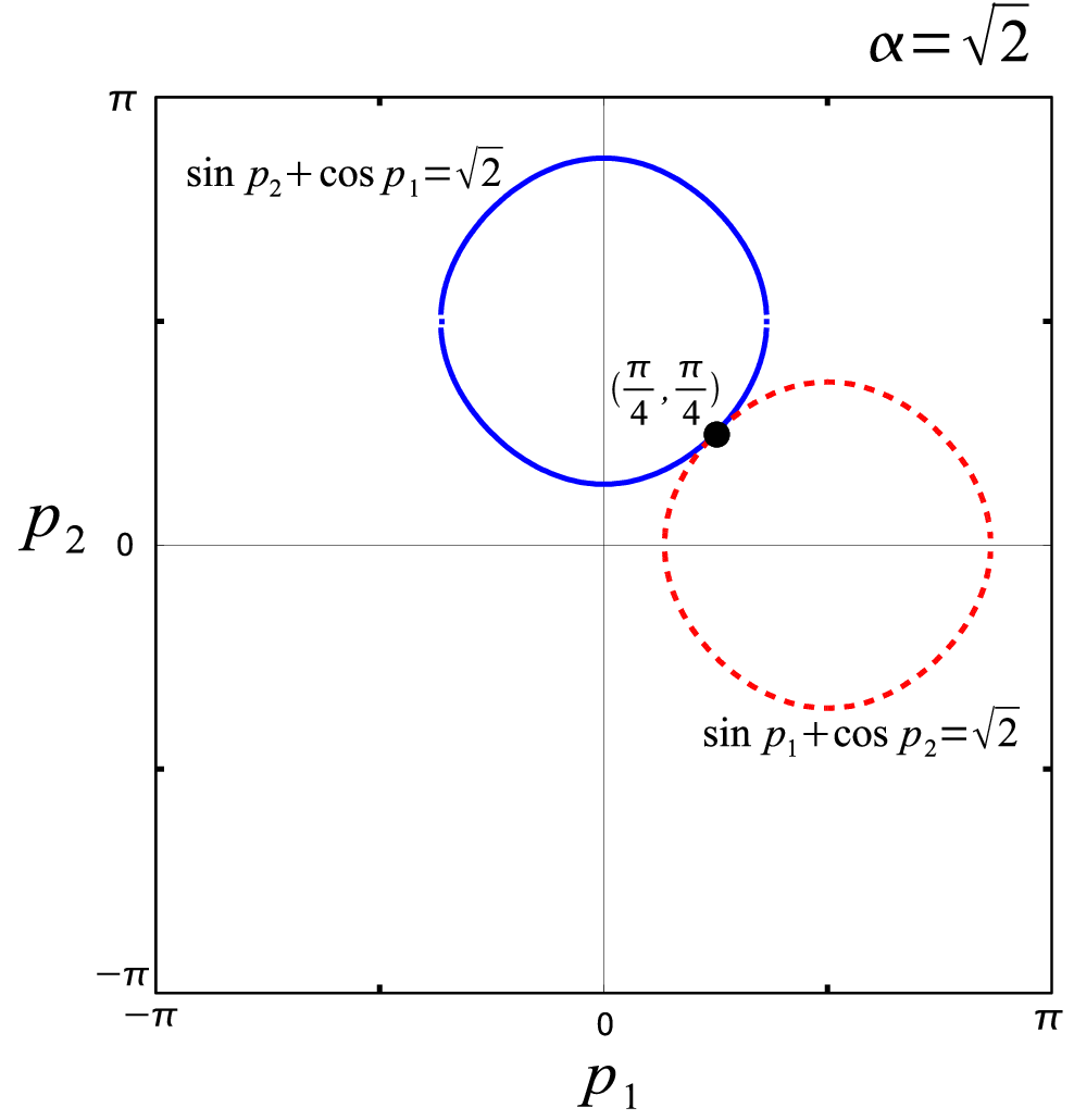
Here only two of the zeros ( and ) remain and the other two are eliminated. Thus the number of species becomes two, the minimal number required by the no-go theorem. As seen from this example, twisting of the order of terms reduces the number of species. We call this method “twisted-ordering” in the rest of this paper. We depict the appearance of zeros in the Brillouin zone for the above two cases in Fig. 1 and 2. The red-dotted and blue-solid curves represent the zeros of the coefficients of and respectively. These curves intersect at only two points for the twisted case in Fig. 2.


Now consider excitations and the physical ()’s at the two zeros. Here the physical at a zero is defined as the product of four coefficient matrices of momenta in the excitation as we will concretely show later. Now the Dirac operator is expanded about the zeros as
| (3) | ||||
| (4) |
Here we expand with respect to defined as and we denote the two expansions as for the zero () and for the other at . Here momentum bases at the zero are given by and while those at the other are given by and . This means excitations from the two zeros describe physical fermions on the orthogonal lattice. And the at , which we denote as , is given by
| (5) |
while the at , which we denote as , is given by
| (6) |
This sign change between the species is a typical relation between two species with minimal doubling since Nielsen-Ninomiya’s no-go theorem requires fermion pairs to possess chiral charges with opposite signs.
II.2 -dimensional case
Now let us go to the -dimensional twisted-ordering method. Here we again start with the following simple action with Wilson-like terms
| (7) |
Here each of the four momentum components can take either or for zeros of this Dirac operator. It means the associated fermion action gives species doublers, the same as for naive fermions.
Then we firstly consider the case with twisting the order of terms once
| (8) |
where we permute the order of and . Here we find that there are zeros of the Dirac operator at
| (9) |
The associated action yields species of doublers. As seen from this example, the twisted-ordering method reduces the number of species also in -dimensions. In this case twisting is performed only once, and the number of species is reduced by a factor of two.
Secondly we permute and in addition to and to give
| (10) |
In this case there are only zeros at
| (11) |
Thus the associated action yields species of doublers. This example indicates that more twisting results in additional reduction of species. In these two examples, Eqs. (8) and (10), twisting is performed partially, and so we call this kind of procedures “partially-twisted-ordering”.
Finally we consider a case that the order of terms are maximally twisted: We permute the terms in a cyclic way to give
| (12) |
In this case there are only zeros at
| (13) |
We have confirmed there are no other real zeros of this operator numerically, and we will discuss an analytical proof in the next section. There are only two species in this case, the minimal number required by the no-go theorem. This is a new type of minimally doubled fermion on the orthogonal lattice.
Now we study the excitations and ’s at the two zeros in a similar way to the -dimensional case,
| (14) | ||||
| (15) |
where we expand the Dirac operator (12) around zeros with respect to defined as and we denote the two expansions as for the zero () and for the other . Momentum bases at the zero are given by , , and while those at the other zero at are given by , , and . This means excitations from the two zeros describe physical fermions on the orthogonal lattice again. And the at , which we denote as , is given by
| (16) |
while the at , which we denote as is given by
| (17) |
This is a typical relation between the two species with minimal-doubling.
Gauging these theories is straightforward. One merely inserts the gauge fields as link operators in the hopping terms for the action in position space. Specifically, for the twisted-ordering minimally doubled fermion in position space we have
| (18) |
where we define
| (19) |
We note that in the twisted-ordering method, we control the number of species by choosing the extent of breaking of discrete symmetries of the action. Twisting of terms leads to breaking of the hypercubic symmetry. On the other hand it is well-known that hypercubic symmetry of the lattice fermion action requires species as shown in [7]. Thus it is reasonable that more breaking of discrete symmetries can lead to less doubling.
III Minimally-Doubled Fermions
In this section we discuss two classes of minimally doubled actions obtained from the original twisted-ordering action (12). The first one, which we call the “dropped twisted-ordering action”, is constructed as following: We drop one of terms in the Dirac operator (12), for example, drop as
| (20) |
This has two zeros given by
| (21) |
Thus the associated action is also a minimally doubled action. Here the two ()’s at the two zeros also have opposite signs
| (22) |
where corresponds to and to . We can also confirm this action describes physical fermions on the orthogonal lattice by looking into excitations from the zeros as in the previous section. We depict the appearance of zeros for the two dimensional case of the dropped twisted-ordering action in Fig. 3. We see there are only two zeros as and . The -dimensional case is similar.

Here we comment on definition of the equivalence of actions. We can convert one fermion action to an equivalent one with a different form by momentum shift and rotation of Gamma matrices. Here the momentum shift means
| (23) |
where are some constant four vector. The rotation of Gamma matrices means
| (24) |
where is an orthogonal matrix. Although by using such a shift and rotation we can control the location of two zeros with the distance and direction between them fixed, the original and transformed actions are clearly equivalent. Now we can easily see the original (12) and dropped twisted-ordering (20) actions never translate into Borici [14] or Karsten-Wilczek [11, 12] actions through these two procedures. It means our actions are independent and new ones.
Next we consider a second generalization where we turn on a parameter in the action (12) as following,
| (25) |
Here we replace unity with a positive parameter in the constant terms of the operator. We will also call this one the twisted-ordering fermion action in the rest of this paper. The case corresponds to the original case. Now, in order to investigate the parameter range within which “minimal-doubling” is realized, we define and rewrite the equations for zeros in terms of these variables
| (26) |
To make it easier to see we rewrite this as
| (27) |
where in principle there are complex solutions. The number of solutions of this system is the same as the original ones (25)(26). Thus we can study the range of the parameter for minimal-doubling by looking into how many real solutions this system of equations has. By eliminating , and , we obtain the following equation for
| (28) |
where we can confirm this by using software such as Maxima. This means, except for , there are only the two solutions
| (29) |
From this should be below so that the solutions are real. For the above equation (28) is satisfied by any value of , which means that zeros appear as a one-dimensional curve, not a point. We will discuss this in detail later. We find there are two real solutions in the range , which corresponds to a pair of minimally doubled species. This is the range of the parameter for minimal-doubling. We can also verify this minimal-doubling range numerically.
What is significant for is that zeros of the Dirac operator (25) appear as an one-dimensional curve, not a point, in the momentum space. We can confirm this as following. Equations for zeros of the Dirac operator (25) at are given by
| (30) |
These equations are satisfied by
| (31) |
where we ignore the arbitrariness of adding . As seen from these relations, the solution appears as an one-dimensional curve. For example, you find the following curve satisfies the above equations:
| (32) |
where can take an arbitrary value. We can also understand this from the fact that (27) reduces to three independent equations for . This emergence of a line solution indicates that the excitation around zeros for a small becomes incompatible with a Lorentz-covariant or a Dirac form. Due to these nonlinear corrections, we conclude that we should use this action only with substantially away from . This property at is also the case for any even number of dimensions.
We can visualize the allowed range of the parameter from the -dimensional analogy. In the d case the upper limit of is illustrated in Fig. 4. For the two zeros join to a double zero, where the excitation is not Lorentz-covariant. For a lower limit, the d analogy shows “Minimal-doubling” persists as long as is positive. We depict d cases for and in Fig. 5 and 6. For the solution appears as an one-dimensional line, thus there is no simple pole in the propagator.
We conclude that the parameter range for minimal-doubling in both and dimensions is given by
| (33) |
In this range two zeros of the d Dirac operator, which we denote as and , are given by
| (34) | ||||
| (35) |
where for convenience we define a parameter as . These two zeros reduce to Eq. (13) with . Excitations from these zeros are given by
| (36) | ||||
| (37) |
where corrections are not negligible for a small as we have discussed. Momentum bases at the zero are given by , , and while those at the other zero are given by , , and . They are clearly non-orthogonal for cases of thus the associated lattices are non-orthogonal as with the Creutz fermion [13].
We note we have confirmed the parameter range for minimal-doubling (33) is also the case with other even dimensions (). From this fact we can anticipate this is a universal property for this class of actions for any even dimensions.


Here we comment on the ranges of the parameter for minimal-doubling in odd dimensions. For example, in the d case, we can rewrite analogous equations for zeros of the operator with , and as
By eliminating and , we obtain the following equation for ,
| (39) |
As seen from this there are two real solutions similar with the d case for as
| (40) |
However, in this case we have six more complex solutions which come from the other factor (39). The question is how many real solutions this equation has. We have studied it numerically and found six real solutions exist below a critical value of as while there are six complex solutions above it. Thus the minimal-doubling parameter range in the d case is given by
| (41) |
In this case the lower limit is non-zero while the upper limit is the same as even dimensional cases. Indeed we can numerically confirm this kind of nonzero lower limit is also the case with any odd dimensional twisted-ordering action. We can explain the reason that there is such difference between the even and odd dimensional cases as following: As seen from (), there are independent equations even for in the ()-dim cases () while there are only equations in the even dimensions for . This means that the Dirac operator can have zeros for in the odd dimensional cases while zeros appear as a curve in even dimensions. Actually, as seen from (39), there are independent real solutions for in the odd dimensions. Since only two zeros exist for also for odd dimensions, there must be a critical point between and in odd dimensions.
IV Symmetries
In the previous section we have studied two classes of minimally doubled actions in (20) and (25), both of which are obtained from the twisted-ordering action in (12). In this section we will discuss discrete symmetries of these actions and redundant operators generated by loop corrections.
Firstly we note both of the actions possess some common properties with other minimally doubled fermions: “gamma-five Hermiticity”, “discrete translation invariance”, “flavor-singlet ” and “flavor-nonsinglet .” The latter is the exact chiral symmetry preventing additive mass renormalization for the neutral pion. In addition to them, they have exact locality and gauge invariance when gauged by link variables. We expect every sensible minimally doubled fermion to possess these basic properties.
On the other hand, Discrete symmetries associated with permutation of the axes and , or invariance depends on a class of the actions. In other words, we can identify minimally doubled actions by these discrete symmetries. Here we show discrete symmetries which the dropped twisted-ordering action possesses:
1. ,
2. ,
3. associated with two zeros.
Here we take the direction as time. We also write the symmetries which the full twisted-ordering action possesses:
1. ,
2. associated with axes permutation,
3. associated with two zeros.
There is also the possibility to utilize the above symmetry in order to recover flavored-, or symmetry. Actually Borici-Creutz action has a flavored- symmetry [17]. However we do not further discuss here details of this point, to which a future work will be devoted.
The dropped twisted-ordering action has and invariance. We consider what redundant operators can be generated radiatively in this action following the prescription shown in [17]. The relevant and marginal operators generated through loop corrections are given by
| (42) |
and
| (43) |
These operators are allowed by the symmetries for possessed by the action. Note that the marginal operators include a renormalization of the speed of light, both for the fermions and the gluons.
On the other hand, the case of twisted-ordering action is similar to that of Borici-Creutz action which has higher symmetry than [17]. It is unlikely that there are more redundant operators generated in the twisted-ordering action than those of Borici-Creutz one shown in [17]. However in the future we need to confirm that this reduction of symmetry does not affect the number of redundant operators. Then we will know whether or not this class is more useful than the Borici-Creutz class.
V Classification
In this section we discuss a classification of the known minimally doubled fermions. So far we have seen four variations on minimally doubled fermions: Karsten-Wilczek, Borici-Creutz, twisted-ordering and dropped twisted-ordering fermions. Here we classify these actions into two types: One of them, which includes Karsten-Wilczek and dropped twisted-ordering actions, is given by
| (44) |
where we take as while as . The point is that indices and are staggered. The different actions in this class depend on the choice for the matrix . For example, consider the following ’s
| (45) | ||||
| (46) | ||||
| (47) |
In the case of (45), the general form (44) reduces to Karsten-Wilczek action as following,
| (48) |
Here you can also add an overall factor as a parameter to . Actually the original Karsten-Wilczek action includes such a parameter in front of terms with a minimal-doubling range of the parameter .
In the case of (46), this reduces to the dropped twisted-ordering action
| (49) |
where you can also add an overall parameter to .
Finally, the action for the case (47) is a new possibility, given by
| (50) |
We see that there are many options associated with possible ’s. One common property with fermions obtained in this way is that two zeros are separated along a single lattice axis and given by and . One significance about the general form (44) is that a coefficient of at least one Gamma matrix has no term. It is also notable that, in a coefficient of each gamma matrix, a momentum component associated with a sine term differs from the component in any cosine term. These two points seem to be essential to minimal-doubling. Here we note minimal-doubling still persists if we add a term to any actions obtained from (44). We can change the location of the two zeros by adding such a term with a parameter.
Here let us comment on a sufficient condition of for minimal-doubling. We found minimal-doubling is realized when you take the following class of ’s: ’s composed by three column vectors as with each vector () taken as , or . All the examples we have shown here satisfy this condition. However we have not yet revealed a necessary condition for this. Our future work will be devoted to revealing such a condition.
The second class of actions includes the twisted-ordering fermion with the parameter and the Borici-Creutz actions. A generalized Dirac operator for this type is given by
| (51) |
where is another set of gamma matrices where we define as an orthogonal matrix with some conditions: At least one eigenvalue of should be and all four components of the associated eigenvector should have non-zero values. Here and has a relation with this as , which means is an eigenvector of as . Thus once is fixed, and are determined up to a overall factor of . By imposing these conditions on , and , the action (51) can be a minimally doubled action. In such a case indicates locations of two zeros as . Adjusting , we can control the locations of the zeros.
Note that the first and second terms in (51) are nothing but naive fermion actions. We can eliminate some species by combining two naive actions with different zeros in one action.
Now let us show this action includes minimally doubled actions. Firstly this general form in (51) reduces to Borici action by choosing , which is given by
| (52) |
where we fix thus is given by .
This general form (51) also yields the twisted-ordering action. For this we take the following matrix
| (53) |
fix , and is given by . Then the general form reduces to the twisted-ordering action with . We can also obtain the case by choosing other values of . For we take along with which an overall factor for changes.
We note this general form (51) also includes non-minimally doubled actions like the partially twisted-ordering actions in (8) and (10). Here let us consider
| (54) |
and fix where is given by . This clearly gives the partially-twisted-ordering action in (10).
Finally we have classified the known minimally doubled fermions into the two types. Now we can derive a lot of varieties from these general forms deductively as we have shown in (50). However the second type of general actions (51) is not restricted only to minimally doubled fermions. We may be able to restrict it by imposing other conditions. We note the two fermion actions which we derived from the twisted-ordering method, namely twisted-ordering and dropped twisted-ordering, belong to different types of minimally doubled fermions although they look similar to each other.
VI Summary
In this paper we study a variety of new classes of minimally doubled fermions and a classification of all the known cases. In Sec. II we propose a systematic method to reduce the number of species, the “twisted-ordering method”. In this method we can choose , , and as the number of species by controlling discrete symmetry breaking. By using this method we obtain new classes of minimally doubled fermions, which we call twisted-ordering and dropped twisted-ordering actions. In Sec. III we study these two classes in terms of the parameter range for minimal-doubling. In Sec. IV we study discrete symmetries of these fermion actions and show twisted-ordering action has symmetry while dropped twisted-ordering action possesses invariance. We also show they require fine-tuning of several parameters for a correct continuum limit because of lack of sufficient discrete symmetries in the known classes. In Sec. V we classify all the known minimally doubled actions into two types. We can derive several unknown minimally doubled actions by this classification.
With several varieties of minimally doubled fermion actions available, a goal is to apply these actions to numerical simulations and study their relative advantages. In particular it is important to investigate how many fine-tuning parameters are required for a good continuum limit and how difficult this tuning is. This kind of study was started in [17]. Recently renormalization of the operators has been also studied in [22, 23, 24]. Both of these studies focused on Karsten-Wilczek and Borici-Creutz fermions. One can now explore other varieties such as ones in this paper. With a better understanding of their properties, one can go on to larger numerical calculations.
Acknowledgements.
TM is supported by Grand-in-Aid for the Japan Society for Promotion of Science (JSPS) Research Fellows(No. 21-1226). TM thanks Taro Kimura for stimulating discussions. MC is grateful to the Alexander von Humboldt Foundation for support for visits to the University of Mainz. This manuscript has been authored under contract number DE-AC02-98CH10886 with the U.S. Department of Energy. Accordingly, the U.S. Government retains a non-exclusive, royalty-free license to publish or reproduce the published form of this contribution, or allow others to do so, for U.S. Government purposes.References
- [1] K. G. Wilson, Phys.Rev.D 10, 2445 (1974).
- [2] H. B. Nielsen and M. Ninomiya, Nucl. Phys. B 185, 20 (1981); Nucl. Phys. B 193 173 (1981); Phys. Lett. B 105 219 (1981).
- [3] D. B. Kaplan, Phys. Lett. B 288, 342 (1992).
- [4] V. Furuman and Y. Shamir, Nucl. Phys. B 439, 54 (1995).
- [5] P. H. Ginsparg and K. G. Wilson, Phys. Rev. D 25, 2649 (1982).
- [6] N. Neuberger, Phys. Lett. B 427, 353 (1998).
- [7] L. H. Karsten and J. Smit, Nucl. Phys. B 183, 103 (1981).
- [8] J. B. Kogut and L. Susskind, Phys. Rev. D 11, 395 (1975).
- [9] L. Susskind, Phys. Rev. D 16, 3031 (1977).
- [10] H. S. Sharatchandra, H. J. Thun and P. Weisz, Nucl. Phys. B 192, 205 (1981).
- [11] L. H. Karsten, Phys. Lett. B 104, 315 (1981).
- [12] F. Wilczek, Phys. Rev. Lett. 59, 2397 (1987).
- [13] M. Creutz, JHEP 0804, 017 (2008) [arXiv:0712.1201 [hep-lat]].
- [14] A. Borici, Phys. Rev. D 78, 074504 (2008) [arXiv:0712.4401 [hep-lat]]; PoS LATTICE2008, (2008) [arXiv:0812.0092].
- [15] M. Creutz, PoS LATTICE2008, (2008) [arXiv:0808.0014].
- [16] A. H. Castro Neto, F. Guinea, N. M. R. Peres, K. S. Novoselov, A. K. Geim, Rev. Mod. Phys. 81, 109 (2009), arXiv:0709.1163 [cond-mat.other].
- [17] P. F. Bedaque, M. I. Buchoff, B. C. Tiburzi and A. Walker-Loud, Phys. Lett. B 662, 449 (2008) [arXiv:0801.3361 [hep-lat]]; M. I. Buchoff, PoS LATTICE2008 (2008) [arXiv:0809.3943].
- [18] P. F. Bedaque, M. I. Buchoff, B. C. Tiburzi and A. Walker-Loud, Phys. Rev. D 78, 017502 (2008) [arXiv:0804.1145 [hep-lat]].
- [19] T. Kimura and T. Misumi, to appear in Prog. Theor. Phys. [arXiv:0907.1371 [hep-lat]].
- [20] T. Kimura and T. Misumi, Prog. Theor. Phys. 123, 63 (2010) [arXiv:0907.3774 [hep-lat]].
- [21] K. Cichy, J. Gonzalez Lopez, K. Jansen, A. Kujawa and A. Shindler, Nucl. Phys. B 800, 94 (2008) [arXiv:0802.3637 [hep-lat]].
- [22] S. Capitani, J. Weber, H. Wittig, Phys. Lett. B 681, 105 (2009) [arXiv:0907.2825].
- [23] S. Capitani, J. Weber, H. Wittig, (2009) [arXiv:0910.2597].
- [24] S. Capitani, M. Creutz, J. Weber, H. Wittig, (2010) [arXiv:1006.2009].