Network Evolution Induced by the Dynamical Rules of Two Populations
Abstract
We study the dynamical properties of a finite dynamical network composed of two interacting populations, namely; extrovert () and introvert (). In our model, each group is characterized by its size ( and ) and preferred degree ( and ). The network dynamics is governed by the competing microscopic rules of each population that consist of the creation and destruction of links. Starting from an unconnected network, we give a detailed analysis of the mean field approach which is compared to Monte Carlo simulation data. The time evolution of the restricted degrees and presents three time regimes and a non monotonic behavior well captured by our theory. Surprisingly, when the population size are equal , the ratio of the restricted degree appears to be an integer in the asymptotic limits of the three time regimes. For early times (defined by ) the total number of links presents a linear evolution, where the two populations are indistinguishable and where . Interestingly, in the intermediate time regime (defined for and for which ), the system reaches a transient stationary state, where the number of contacts among introverts remains constant while the number of connections is increasing linearly in the extrovert population. Finally, due to the competing dynamics, the network presents a frustrated stationary state characterized by a ratio .
pacs
05.20.-y,05.65.+b,89.75.Hc1 Introduction
In the last decade, it became clear that the statistical properties of natural or artificial networks differ most of the time from the properties of random graphs. Nowadays, it is well known that the formation and the dynamics of complex networks are far from random but are governed by underlying organizing principles. Some of the most famous networks are: the living cells (formed by chemical and chemical reactions), the internet, the world wide web, power grids and social networks. See [1, 2, 3, 4, 5, 6] for review articles. In addition, it appears that networks are an interesting support for various dynamical processes where the topology should play a crucial role. As an example, the random walk [7, 8, 9, 10, 11, 12] or the process of synchronization in complex networks [13, 14] has been some of the favorite playgrounds of the scientific community. One should also mention the spread/diffusion of ideas, innovations or viruses [15, 16] that are of particular importance. These dynamical problems have been studied on regular [17, 18], random [19, 20, 21], small world [22, 23, 24, 25, 26, 27, 28] and scale free networks [29, 30].
A challenging task, in the characterization of the network topology is the detection of sub-units [31, 32, 33, 34, 35, 36, 37], called clusters, modules or communities. These are the signature of the hierarchical nature of complex systems [38, 39, 40]. In the case of social networks [41] and in the framework of epidemiology, the spread of an infectious disease within a community and its transmission between communities is a key to understand and prevent pandemic outbreaks. Interestingly, while for random graphs, epidemiological models present a disease free state below a critical infection rate, it has been shown, for scale free network, that any spreading rate leads to the infection of the whole network [42, 43]. In an effort to build realistic models, epidemiologist focused on understanding the robustness of the results to the model assumptions [44]. Finding out the simplest microscopic rules of a social network is a difficult task and is strongly dependent of the population under consideration. Networks that include social communities, social distance and group structures have been proposed [45, 46].
Motivated by the sociological interaction amongst extroverts and introverts, we analyze the dynamical properties of a finite size network composed of two populations. In an epidemiological context, we believe that the daily network of interactions is not necessarily scale free. We propose an alternative dynamics of the preferential attachment rule, where the populations are characterized by a ‘preferred degree’, respectively and for extroverts and introverts. In our model, each individual tries to reach the ‘preferred degree’ through the possibility to create or destroy bonds. The succession of these microscopic events governs the dynamics of the entire network. Evidently, the growth of the network is subject to the constraint imposed by the preferred degrees. Such constraints are known to lead to single scale networks [47]. Examples are found in actors collaborative networks which present a exponential cutoff of the degree distribution.
We study the time dependence of such a network, starting with no contacts and evolving through birth, growth and relaxation. We find three regimes separated by two characteristic times and associated to the preferred degree and , respectively. In the early time regime, the two populations are indistinguishable while the second time regime is understood as a relaxation towards a transient stationary state. In this state, the number of links between extroverts is linearly increasing while the number of introvert-introvert and introvert-extrovert links are constant, depending on the difference of the population sizes. In the last time regime () the system relaxes towards the final, stationary state. Not surprisingly, the competing dynamics between the two populations induced frustration in the stationary state. This results simultaneously of the creation of cross-population links from the extrovert population and of their destruction by the introverts.
The paper is organized as follows: we start, in section 2, with a presentation of the model, introducing the probability to create a link as a function of the system parameters. In section 3, we give successively a full and coarse-grained description of the dynamics of our network through the master equation defined in the complete and reduced configuration space. To pursue our analysis further, we derive, for finite system, the mean field equations describing the time evolution of the average degree of each population. In section 4, starting from an empty network we study the evolution of the network through the early, intermediate and late time regimes. For various parameter values, the prediction of the mean field theory (in the limit ) are compare to Monte Carlo simulation data. The limitations of our approach are presented in section 5, especially in the intermediate time regime where the system presents unexpected finite size effects. We summarize our results in the last section and discuss possible extension of our study.
2 The model
Generally, a realistic network is composed of an arbitrary number of populations or groups. In our work, motivated by the competing aspect of different populations, we focus our attention on the interaction between just two groups: extrovert and introvert individuals. The model under consideration is composed of nodes divided in two populations, respectively (extrovert) and (introvert), of size and with being constant. Each group is characterized by its preferred degree and . Extrovert and introvert individuals prefer to have respectively many and few contacts, which is modeled by imposing . It is the succession of local events, such as creation or destruction of edges by each individual, that governs the dynamics of the entire network. Starting with a totally disconnected network (i.e., zero contacts), we study the growth of connections induced by the microscopic rules. Of course, more sophisticated versions, including the birth and death process of nodes or “mutation” from one group to the other, can be considered.
In our simulations, one time-step is defined by the successive random selection of individuals where each node is updated once, according to the rules detailed below. Defining
| (1) |
the probability to select a node of the population is given by (and for ) such that on average, all nodes are updated once in each time-step. We will label a node by , denote its social group by (), and its actual degree by . When a node is chosen, we will create or destroy a link attached to it, with respectively probability or . For simplicity, we will choose the same structure of the probability of creation for the two groups. The only difference being the preferred degree, , which enters through the dependence on in terms of the ratio
| (2) |
Clearly, we must insist that if the degree , since there can be no more links to destroy. On the other hand, a natural condition is if . The crossover from to can be characterized by some width, which we also introduce as a parameter: . We may regard this as a measure of the ‘flexibility’ or ‘tolerance’ level of the population, with larger corresponding to higher ‘rigidity’ or lower ability to tolerate a degree far from the preferred value. Specifically, we choose
| (3) |
and denote, for the node ,
| (4) |
as the probability to create a new link with a randomly chosen individual who is not already in contact with . On the other hand, with probability , we randomly choose one of its existing links to destroy. After the update, its degree is simply , a restriction which can be easily lifted in future studies.
Clearly, form equation (3), the ‘width’ of the crossover region decreases with , so that approaches the Heaviside function in the limit . Much of our analysis will be based on this limit and its associated predictions for the system’s behavior are expected to be universal. Note that the probability is the familiar Fermi-Dirac distribution, by identifying with . In our context, it has another advantage, namely, the ratio of destruction to creation probabilities is a simple power of : . Other choices for are of course possible. However, we believe the detailed specifics of will lead to only non-essential properties displayed by the system. For most of our simulations we choose: , , , , and various ’s in the interval .
3 Master equations and a mean-field approach
3.1 Full description of the system
Such interwoven systems are particularly well described by the powerful approach and tools of statistical mechanics. It is clear that only few exact results can be extracted and that an analytical description remains challenging. The size of the configuration space illustrates perfectly the complexity of networks related problems. We start by defining the contact variables between the nodes and , such that if a link connects these points and otherwise. As we exclude ‘self-links’ in our model, at all times. Thus, a configuration, , is uniquely labeled by the symmetric (off diagonal) ‘matrix’ . Since there are elements in such matrices, there are possible configurations (i.e., ). The master equation of the probability to find the system in a particular state at a time , has the usual structure
| (5) |
where is the probability to make a transition from to . Note that here, is not a time-step as defined above, but a single attempt to update the network. Since one link is always created or destroyed, the probability for any to remain unchanged is zero. Of course, it is possible to write an explicit expression of the probabilities in terms of the elements of the set . However, this approach is intractable and so, we will not pursue it further. We will consider simpler approximations below.
3.2 Reduced phase space
Instead of the detailed picture above, we believe most of the essentials of this network will be captured by a coarse-grained view, namely, a dimensional phase space spanned by (), the total number of links between extroverts (introverts), and , the total number of links between the two groups (see Fig. 1). Defining as the probability to find the system in a macrostate defined by the triplet , its master equation takes the following form
| (6) | |||||
where and are the probabilities to create and destroy a link of type (). Even in this simplified picture, the exact transition probabilities () during one time step are not easy to write, since that would require the knowledge of how the and links are distributed in the system. To proceed, we assume that all the nodes of the same population have the same degree, so that only their averages, denoted by (), enter into our . Clearly, the degrees and receive contributions from links within the groups and and those across groups (). Specifically, defining the restricted degree by
| (7) |
we have
| (8) |
From these, we write the ratios and construct the creation probabilities:
| (9) |
Let us emphasize, instead of having individual ’s, we deal with only two “group” ’s here: and . Next, noting that the creation of a link by an individual requires the random selection of another node not already connected, we will approximate that probability by
| (10) |
Thus, within the group and , the probabilities and are given by
| (11) |
Note that the probabilities () depend on only two of the three variables (,,). Following the same lines and defining , we arrive at
| (12) |
where is the probability to pick, among the existing links, a link connecting a node of the same population. Finally, for the creation and destruction of cross-links, we have
| (13) | |||||
| (14) |
As usual, if is known, it can be used to find the averages of all observable quantities. A relevant example is given by the average degree associated with each population at any time :
| (15) |
For convenience, we will drop the subscript in below, except when its presence is needed for clarity. We will also discuss time independent (or almost so) quantities, which will be denoted by a suitable superscript (e.g., ).

3.3 A mean-field approach
Even in the reduced phase space, the master equation (6) cannot be solved exactly. To gain some insight into our system, we proceed with a mean-field approximation (i.e., replacing averages of functions by functions of averages). In this process, we will often encounter creation probabilities that depend on . Therefore, let us define for convenience
| (16) |
From the exact equation , we find
| (17) |
which, recalling and rescaling , leads to
| (18) |
and similarly
| (19) |
The equation for the restricted degree is also straightforward, though slightly different:
| (20) |
With the equations
| (21) |
we have a closed set of three ordinary, nonlinear differential equations for three functions: . Of course, we can make linear combinations of the above to write equations for and . However, this two equations do not close since both involve . One instructive combination is given by
| (22) | |||||
which is the related to the total number of links in the entire system by the relation . Its evolution is governed by
| (23) | |||||
A convenient simplification occurs if we take the limit , namely,
| (24) | |||||
| (25) | |||||
| (26) |
In the following, we will investigate the time evolution of these quantities, using both Monte Carlo simulations and the equations above.
4 Time evolution
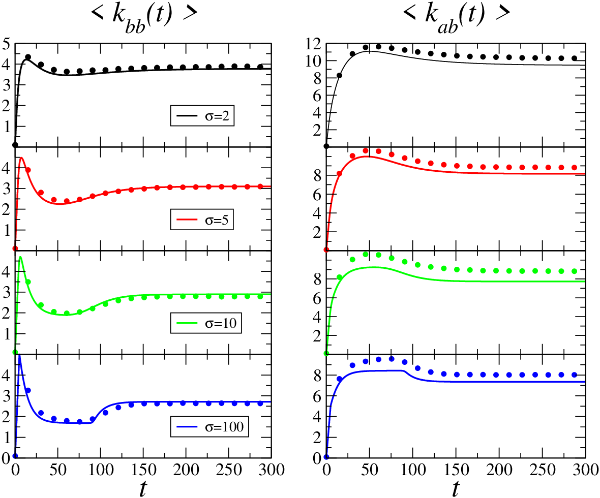
In this section, we present the studies of how an initially empty network evolves to the steady state. Such a scenario may be realized when the population is formed from a collection of ‘complete strangers,’ such as at the start of a cruise or the beginning of a school year (for, e.g., kindergarteners or college Freshmen). Simulating the network according to the rules above, we discover three time regimes, as well as non monotonic behavior in the time evolution of the restricted degree and . See figure (2). As we will show, the different regimes can be understood in terms of the mean-field approach. In particular, provided the ’s are well separated, the characteristic times ( and ) separating these regimes become quite well-defined for systems with large . Such cases correspond to a highly ‘rigid’ population, for which both creation and destruction of links are highly probable even for small values of . We will analyze the three regimes successively, for a range of values of the system parameters.
4.1 Early time regime
In the early time regime, the network is nearly empty, so that the probabilities of creation of links are close to unity. Then, the average number of links () grows linearly with and it is easy to find the slopes for each of the three classes of links. In the limit , the probabilities of creation become Heaviside functions and we can define the early time regime by the times , in which . Equation (23) simply leads to while (24), (25) and (26) predict trivially
| (27) |
We can include finite population size effects and use (18-20) to obtain rounding of this linear growth. In this regime, we should note that defined by the ratio , is time-independent and given by
| (28) |
with =1. Remarkably, even if the size of the populations are different (), the growth of the degrees of the two groups are indistinguishable:
| (29) |
a result that breaks down for and . Now, we see the meaning of : It marks the time when the introverts reach their ‘tolerance’ level, i.e., . Thus, we have
| (30) |
If we include finite effects, then this becomes . In figure (3) and (4) these results are compared to the Monte Carlo simulation data. The short time evolution of the restricted degrees, , are plotted for . The linear increase of the degrees is in perfect agreement with our predictions. The comparison for various values of are shown in Fig (4). In the latter figure, we plot the time derivative of the degrees at time (, and ) as a function of . Agreement between theory and simulations is again excellent.


4.2 Intermediate time regime
Similar to considerations above, let us define by the condition which satisfies the extrovert population. In the regime, , with (and relatively small ), the behavior of the system is characterized by two competing tendencies. The extroverts have yet to reach their preferred connectivity and so, continue to attempt creating links. Since some of these will be cross-links (), the introverts find themselves having more connections than the preferred level and tend to destroy links. In the case , we can expect and the nature of this intermediate ‘state’ is more exposed. In particular, a very large system (e.g., ) may reach a ‘steady’ state, in which the extroverts continue to create links at a constant rate. On average, a constant fraction of these new links will be cross-links, which are then destroyed by the introverts. In such a state, the rate of creation of cross-links by the extroverts balances the rate of destruction by the introverts. Thus, both restricted degree and remain essentially constant, values which will be denoted by and . The continued growth in must be entirely through that in (which is ). Finally, the end of this regime is marked by the extroverts reaching their preferred . We can estimate through with
| (31) |
We will show that , and so, for , we find
| (32) |
In the remainder of this subsection, we will demonstrate that this scenario is borne out, at least qualitatively.
Remaining with the simple (but extreme) case of and approximating the creation probability for the extroverts by unity (i.e., ) leads to a consistent solution. By ignoring terms with , formally decouples and we need to solve a system of only two variables, i.e., and . Specifically, equations (24), (25) and (26) reduce to
| (33) |
and
| (34) | |||||
| (35) |
Since the dynamics of the extroverts decouples (except through an external, “source-like” term in the second equation), it is sensible to consider an equation for in lieu of (35):
| (36) | |||||
| (37) |
Since is a function of alone, the latter equation together with equation (34) form an explicitly closed set. At large times, we have the solution
| (38) |
where the superscript (⋆) denotes (quasi-) stationary values of the relevant quantities. In particular, eliminating the last terms from equations (34) and (37), we easily find
| (39) |
and so, for ,
| (40) |
Notice that these results are ‘universal’ in that they do not depend on the explicit form of the probability of creation (3), but only on its being well approximated by a Heaviside function. The interpretation of the latter is particularly appealing. The introverts are satisfied, as far as their overall degrees are concerned. The only dynamics left in this regime is a redistribution, from cross-links () to intra-group links (). Before the (quasi-) stationary state is reached, the increase of cross-links are, of course, driven by the extroverts (trackable to the first term in equation (35)).
The other (quasi-) stationary values follow readily:
| (41) |
with the ration and . In the lowest panels of figure (2), for which , and , this (quasi-) stationary state is well represented, in the range . The solid lines are results of numerical integration of the full set of equations (24), (25) and (26). They confirm this scenario quite well. An example is the ratio . The dots are results from simulation. Clearly, there is also qualitatively good agreement, especially considering what a drastic approximation went into formulating this simple theory.
4.3 Late time regime
The onset of the last time regime is characterized by the following. While finally the extroverts reach (on average) their preferred degree , the system is not completely “satisfied” as the introverts have been driven, up to this time, by the zealous creation of cross-links from the extroverts. Thus, readjustments will take place, through mostly the destruction of cross-links. The decrease of the number of cross-links in turn affects the introverts, who compensates by creating more links. Again, the last panels of figure (2) showcase this scenario quite well, starting at . With both degrees being mostly satisfied, the two populations spend this final time period readjusting the distributions of cross-links and intra-group links, until the true stationary state is reached.
Let us denote the relevant quantities of the final state by a superscript (∗), and seek the solution to . Again, for simplicity, we present the results in the limiting case . First, considering (23), we find
| (42) |
This equation expresses a universal, and intuitively understandable, aspect of the stationary state. Dividing both sides by , the left can be recognized as the probability to create a link in the system, regardless of which group the individual is a member. Therefore, equality (42) simply states that this probability must be . The other equations for and can be obtained by rewriting the right hand sides of :
| (43) | |||||
| (44) |
Since and are uniquely related to each other (and similarly for and ) one has
which provides the necessary second equation between and . Note that, like equation (42) this does not depend on the explicit functional forms of the probability . To continue further, we can recall the explicit forms, such as , or consider the limit , in which we simply have, regardless of the details of ;
| (46) |
Then, the only parameters which control the fixed point are
| (47) |
which appear as coefficients
| (48) | |||||
| (49) | |||||
| (50) |
in a quadratic equation for :
| (51) |
A similar equation is easily obtained for , by replacing . The solutions are readily found, though the expressions do not convey clear messages. To gain some insight, we consider two simple limits: and .
- Of course, the physics of is trivial, since the system consists of two identical populations (). Thus, and . Here, represents an arbitrary partition (perhaps based on other attributes) of a homogeneous population. We find easily from considering the fraction of the average degree , say, that are connected to the “introverts,” i.e., . But, from equation (8) this fraction is , so that
| (52) |
Naturally, this is also the result if we consider the fraction of connected to the extroverts. From this, it follows immediately .
- On the other hand, if the two populations are of the same size () but distinct (), the results are slightly less trivial:
| (53) | |||||
| (54) |
An interesting, and somewhat unexpected result is obtained for the limit (), in which the average number of links within the group of introverts, , approaches a finite fraction of . From the above, we have
| (55) |
so that only a quarter of an introvert’s connections are with other introverts. Again, the ratio appears to be an integer: . The dynamics in this scenario may be referred to as “frustrated” and described as follows. In their attempt to establish large number of contacts, the extroverts are just as likely to hit upon the introverts and so, to increase . But this activity is not welcome by the introverts and links would be cut in response. If an introvert were connected to just as many cross-links as intra-group links, then both and are equally likely to decrease. But such a situation cannot be sustained, since only the cross-links are continually being formed (by the extroverts). Thus, there must be more cross-links for a sustainable balance to emerge. Examining the last panels of figure (2) again, we see that this ratio is quite consistent with the large behavior of simulation data. It would be useful if a simple and intuitive argument can be advanced to arrive at the ratio .
With a good grasp of the final stationary state we obtain a general picture of the relaxation dynamics through the standard linear stability analysis. Defining the vector , with , one easily obtain the expression of the matrix that governs its evolution: . Three relaxation times emerge, given by the inverse of the eigenvalues of . In the limit , a careful examination reveals that the largest relaxation time , which governs the asymptotic behavior, is of order one while the two remaining characteristic times scales as . The details of this analysis can be found in appendix. With more effort, we can compute the precise value of and compare the tail to those in simulations. However, we doubt that such an exercise will provide any further insight, since we expect the agreement between a mean field approach and the fully stochastic problem to be good only at a qualitative level.
5 Limitations of mean field theory
From the previous section, we see that the simple minded, mean-field approach (with large ) provides a good qualitative picture of the evolution of our network. On the other hand, it is also clear that there are limitations, which are not easily anticipated. This section is devoted to a brief description of some of the shortcomings and speculations on the missing crucial ingredients.
5.1 Drifts in the intermediate regime
From our simulation data, with and , we observe a slow drift – that scales with – in all quantities associated with the introvert population, e.g., , etc. Most significantly, both and drift with . But, in a mean field approximation, the latter probability (which is ) is replaced by and so, becomes intimately related to . In particular, if , small changes in would induce drastically magnified (or suppressed) changes in . Examining figures 5 and 6, it is clear that the drifts in these quantities are comparable, rather than (or ). Such results are clear signals that correlations like are non-trivial. Even if we ignore such difficulties and examine the corrections in the mean field equations (18-20), we can show that they cannot produce a consistent set of results that includes a linear dependence with coefficients. A more interesting behavior is the scaling of the restricted degree with the size of the population. By choosing the origin to be and using the scaled variable , the data for all the ’s can be collapsed (shown in the inset in figures 5 and 6). Given that mean field theory cannot even predict a linear drift, we believe that an explanation of scaling can only emerge with a better understanding of the stochastics. To initiate further studies along these lines, one of us (RZ) has investigated the distribution of degrees for the simplest version of this model possible – single population, – and found it to be an exponential [48]. We believe that such non-trivial distributions will provide some the crucial ingredients needed to establish a theory for both the existence of these slow drifts and their scaling functions.
5.2 Finite effects and universality for large
With moderate ’s, the creation/destruction probabilities are rounded, so that mean field theory predicts smoother transitions between the regimes. This rounding is especially pronounced for the second transition, . As can be seen in figure (2), this transition is obscured even for , displaying only smooth, non-monotonic behavior. In other words, finite rounding in the theory becomes significant when drops below . By contrast, the noise in the simulations completely masks this transition, even for . At the same time, (apart from a constant off-set) the three sets of data with are essentially identical through this transition. Again, we view such differences between predictions and simulations as limitations of the mean field theory.
Another interesting aspect of finite is ‘frustration.’ Since everyone is more ‘flexible,’ the extroverts/introverts can tolerate a finite level of cross-links being destroyed/created by the other group. As a result, and , as seen in simulations. Naturally, also plays a role. In general, the theory above predicts . Given etc., we see that the ratios will differ from unity for finite . We can gain some insight by rewriting equation (42) in a manifestly symmetric form:
| (56) |
Clearly, the two ratios lie on opposite sides of unity. By computing their precise values, we see that they agree reasonably well with data (e.g., for in figure 2). In this connection, we note that the agreement is much better for intra-group links (e.g., ) than for the cross-links. Presumably, this aspect is also a limitation of mean field theory.


6 Summary and outlook
Motivated by the competing dynamics of different social groups, we analyzed the birth, growth and relaxation of a network formed by two populations. The main distinction between these two is their preference for having different degrees: and . With a society of extroverts and introverts in mind, we considered mainly systems with and . In our study, we focus only on the evolution of the network, i.e., the connections between individuals. In particular, during each time-step of our simulation (defined by the random selection of individuals), we count the degree () of each node to determine the probability to create or destroy a link (, ). In this work, we chose , which is effectively a Fermi-Dirac function, starting at , dropping monotonically with through over a range controlled by . In this manner, if the degree of the selected node is too low, it creates a link with a randomly picked new “friend.” On the other hand, if its degree is too high, a random chosen link is cut.
Performing computer simulations, we evolve an initially unconnected set of individuals, with a variety of ’s and ’s. All data collected reveal three time regimes, characterized by non-monotonic behavior of the introverts’ degrees. In the early regime, all individuals are creating links, so that the connectivity in both groups grows linearly. The onset of the intermediate regime is signaled by the introverts reaching their preferred degree while the extroverts remain unsatisfied. Not surprisingly, the cross-links continue to be created by the latter. The introverts struggle to cut links, but, doing so at random (in our model), find themselves with more cross-links than a sustainable value. In other words, the cross-links overshoot, while the introvert-introvert links undershoot. Finally, the late regime is characterized by the extroverts having reached their preferred degree, so that the final, stationary state is reached through the redistribution between intra-group links and cross-links. To describe these scenarios with more than words, we turn to various theoretical approaches.
A full description of the system can be formulated by a master equation for , where / corresponds to the absence/presence of a link between individuals and . Though we can write such an equation, we cannot solve it. Instead, we consider an approximate formulation, using only three “global” variables: (), the total number of links between the extroverts (introverts) and , the total number of cross-links. Even in this reduced phase space, we cannot solve the master equation exactly. To make progress, we exploit a standard mean field approach, writing equations of evolution for the average degrees within each population ( and ) and those associated with cross-links: . The emergence of the three time regimes can now be predicted and qualitatively good agreement between theory and simulations are found. Surprisingly, in the case , the ratio of the restricted degrees and is given by an integer in the asymptotic regime of both transient and stationary states. Of course, there are limitations to this crude theory, some of which we duly noted.
Our study should be regarded as the first step towards a fully interacting adaptive network, in which the individuals are characterized by some states (e.g., opinions, susceptible/infected, etc.) as well. In this work, only the links are endowed with dynamics. Even so, there are many unanswered questions which deserves being pursued. Exploring ways to go beyond mean field theory, by studying the full distribution in , is just an example. Work on this aspect is in progress and will be presented elsewhere [48]. Having more than two groups is another. In reality, every individual will have its own preferred degree () or flexibility (), which generates an interesting problem with quenched disorder. Needless to say, we can study further variations, each incorporating more aspects of real social networks.
If we endow individuals with states and their dynamics, then the vistas are even wider. Since one of our motivations for the present study is how epidemics can be affected by social behavior, let us provide a simple example by considering the epidemiological model on such a dynamic network. See [49] for a review of the basis of epidemiological theory and network theory. In this framework, models that involve adaptive networks have been considered in [50, 51, 52], where the networks “rewires” by having nodes shifting their connections from one friend to another. If we admit the simplest psychology and let the preferred degrees depend appropriately on the level of the epidemic (through the total fraction of infected individuals, say), we can expect oscillations to occur. Promising preliminary results have been obtained [53] for a much simpler version. In that model, mean field theory predicts only fixed points with no limit cycles (though underdamped oscillations can occur). Simulations which include stochastics show only a simple stationary distribution, although a signature of the feedback induced oscillations can be found in the autocorrelations (and its power spectrum [54, 55]). In this regard, we believe that novel and interesting phenomena will emerge if feedback is introduced into the system by coupling of the dynamics of the nodes with that of the links. If realized, such a system will have its own natural frequencies (periods) that depend only on the system parameters. How these “internal” periods interact with those from “external” drives (e.g., seasonal variations of infectious diseases) will surely be of interest in the modeling of epidemics in interacting populations.
7 Appendix: Linear stability analysis
For our analysis, we consider the limit only, i.e., equations (23), (24), (25) and (26). For convenience of notation, let us define
| (57) |
so that
| (58) |
Therefore, for arbitrary and , we have
| (59) | |||||
| (60) |
A useful guide is to keep in mind our specific case, in which and showing explicitly the nature of these derivatives. Let us write the equations for and as
| (61) |
where and with
| (62) |
For , one obtains
Defining the vector
| (64) |
and linearizing equations (24), (25) and (26) around the fixed point, we write
| (65) |
We see that every element of will contain or (or both), which are . Denoting this order by we have
where
denote the above functions at the fixed point. In the large limit of interest here, the simple expectation is that all eigenvalues will be proportional to . However, this would lead to an instantaneous relaxation into the steady state (i.e., with decay time). A more careful examination reveals that has a zero eigenvalue, with eigenvectors
with
| (75) |
Since both its trace and its co-factor (respectively, and ) are non-zero, the other two eigenvalues are . Expecting both to be positive on physically grounds, we do not pursue their precise values.
Given that we have the eigenvectors at , we can compute the eigenvalue at by standard perturbation theory. Calling that part of the matrix , the eigenvalue is given by standard perturbation theory:
| (76) |
where is the terms in . The decay of any quantity that has overlap with will be independent of in the large limit.
Acknowledgements
We thank S. Dorosz, B. Schmittmann, and L.B. Shaw for illuminating discussion. This research is supported in part by the US National Science Foundation through DMR-0705152.
References
References
- [1] Steven H Strogatz, 2001 Nature 410 268
- [2] Réka A and Barabási A L, 2002 Rev. Mod. Phy. 74, 47
- [3] Dorogovtsev S and Mendes J F F, 2002 Adv. Phys. 51 1079Ð1187
- [4] Newman M E J, 2003 SIAM Rev. 45 167Ð256
- [5] Boccaletti S et al, 2006 Phys. Rep. 424 175Ð308
- [6] Costa L d F et al, 2007 Adv. Phys. 56 167Ð242
- [7] Hubermann B et al, 1998 Science 280 95
- [8] Kleinberg J M, 2000 Nature 406 845
- [9] Adamic L A, 2001 Phys. Rev. E 64 046135
- [10] Bilke S and Perterson C, 2001 Phys. Rev. E 64 036106
- [11] Burda Z et al, 2001 Phys. Rev. E 64 046118
- [12] Noh J D and Rieger H, Phys. Rev. Lett. 92, 118701
- [13] Wah Wu C, 2007 Synchronization in complex networks of nonlinear dynamical systems, World Scientific Publishing Co. Pte. Ltd., London
- [14] Arenas A et al, 2008 Physics Reports 469 93-153
- [15] Coleman J et al, 1957 Sociometry 20 253
- [16] Valente T, 1995 Network Models of the Diffusion of Innovations, Hampton, Cresskill, NJ
- [17] Kauffman S A, 1993 The Origins of Order, Oxford University, New York
- [18] Keeling M J, 1999 Proc. R. Soc. London, Ser. B 266 859
- [19] Solomonoff R and Rapoport A, 1951 Bull. Math. Biophys 13 107
- [20] Rapoport A, 1957 Bull. Math. Biophys. 19 257
- [21] Weigt M and Hartmann A K, 2001 Phys. Rev. Lett. 861658
- [22] Moukarzel C, 1999 Phys. Rev. E 60 R6263
- [23] Newman M E J and Watts D J, 1999 Phys. Lett. A 263 341
- [24] Newman M E J and Watts D J, 1999 Phys. Rev. E 60 7332
- [25] Moore C and Newman M E J, 2000 Phys. Rev. E 61 5678
- [26] Moore C and Newman M E J, 2000 Phys. Rev. E 62 7059
- [27] Newman M E J et al, 2000 Phys. Rev. 84 3201
- [28] Kuperman M and Abramson G, 2001 Phys. Rev. Lett. 86 2909
- [29] Johansen A and Sornette D, 2000 Physica A 276 338
- [30] Tadić B, 2001 Eur. Phys. J. B 23 221Ð228
- [31] Blatt M et al, 1996 Phys. Rev. Lett. 76 3251
- [32] Zhou H, 2003 Phys. Rev. E, 67 061901
- [33] Reichardt J and Bornholdt S, 2004 Phys. Rev. Lett. 93, 218701
- [34] Newman M E J, 2004 Phys. Rev. E 69 066133
- [35] Newman M E J, 2004 Eur. Phys. J. B 38 321
- [36] Palla G et al, 2005 Nature 435 814
- [37] Derényi I et al, 2005 Phys. Rev. Lett. 94 160202
- [38] Ravasz E et al, 2002 Science, 297 1551
- [39] Vicsek T, 2002 Nature 418 131
- [40] Guimerá R et al, 2003 Phys. Rev. E 68 065103
- [41] Watts D J et al, 2002 Science 296 1302
- [42] Pastor-Satorras R and Vespignani A, 2001 Phys. Rev. Lett. 86 3200
- [43] Pastor-Satorras R and Vespignani A, 2001 Phys. Rev. E 63 066117
- [44] Halloran M E et al., 2008 PNAS 105(12) 4639
- [45] Noh J D et al, 2005 Phys. Rev. E 71 036131
- [46] Boguna M et al, 2004 Phys. Rev. E 70 056122
- [47] , Amaral L A N, et al., 2000 Proc. Natl. Acad. Sci. U.S.A. 97 11 149
- [48] Liu W J, Schmittmann B, and Zia R K P, to be published 2010
- [49] Keeling M J and Eames K T D, 2005 J. R. Soc. Interface 2 295-307
- [50] Gross T et al, 2006 Phys. Rev. Lett. 96 208701
- [51] Shaw L B and Schwartz I B, 2008 Phys. Rev. E 77 066101
- [52] Schwartz I B and Shaw L B,. 2010 Physics 3 17
- [53] Platini T, to be published
- [54] Alonso D et al, 2007 J. R. Soc. Interface 4 (14) 575-582
- [55] Simes M et al, 2008 J R Soc Interface 5 (22) 555-66