Theoretical Analysis of a Large Momentum Beamsplitter using Bloch Oscillations

The Bloch oscillation acceleration is based on coherent transfer of momentum between an accelerated optical lattice and atoms. The optical lattice results from interference of the two lasers beams of the same intensity $I$, detuned by $\Delta$ from the one photon transition. The amplitude of the resulting standing wave is $4I$. Atoms endure a periodic potential $U(x)$ due to light-shift (a.c. stark effect) which can be expressed as:

where $k=2\pi/\lambda=2\pi\nu/c$ is the wavevector of the laser, $U_{0}=h\frac{\Gamma^{2}}{8\Delta}\frac{I}{I_{S}}$ with $\Gamma$ representing the natural linewidth of the excited state and $I_{S}$ its saturation intensity. In the following, the constant part $U_{0}/2$ which does not play any role for the explanations is removed from every equation. Because of the periodicity of the potential, the eigenenergies of the system show a band structure [15]. Each eigenstate is described by a band index $n$ and a quasimomentum $q$ defined modulo $2\hbar k$ [16]. The Fig. 1 represents this band structure, where the first Brillouin zone is unfolded. The splittings between bands at the center ($q=0$) and at the edge ($q=\hbar k$) of the first Brillouin zone occurs where atoms are resonantly coupled by $U(x)$.

In a quantum optics view, the avoided crossing (Bragg resonance) between the first and second bands is connected to the resonance of the two photon transition between states of momentum $p=\pm\hbar k$. Similarly, the splitting between the second and third bands is due to a resonant four photon transition between states of momentum $p=\pm 2\hbar k$, and so on for the $n^{\mathrm{th}}$ and $(n+1)^{\mathrm{th}}$ band. The order of the transition grows with the band index, thus the higher the band index is, the weaker is the splitting between the bands.

When the atoms in the first band are subjected to a constant and uniform force, their quasimomentum increases linearly with time. If the force is weak enough to induce adiabatic transition, the atoms stay in the first band and therefore have a periodic motion (Bloch oscillations [17]). The time necessary for a variation of the quasimomentum of $2\hbar k$ is the period of the oscillations. For atoms in higher band, for a constant acceleration, the probability to make an adiabatic transition (stay in the same band) will be higher for low values of the band index.

Bloch oscillations were initially introduced in the case of a lattice and a uniform force. In our experiment, a constant acceleration is applied to the lattice. This acceleration acts like a force in the frame of the lattice (see Ref. [12]), and an equivalent of Bloch oscillations can be observed [14]: the adiabatic transition corresponds to a change of velocity of 2 recoils, whereas a non-adiabatic transition does not change the velocity of the atom (free particle).

In our LMTBS, one wavepacket is loaded in the first band (A, see Fig. 1) and the second in the third band (B). The acceleration is small enough so that atoms in the first band are likely to make an adiabatic transition, but strong enough so that atoms initially in the third band change band. The atoms in the first band are periodically accelerated by 2 recoils momentum. In the same time, atoms in the third band are not accelerated. This process allows us to selectively accelerate atoms depending on their initial velocity.

Note that in our experiment, atoms with different velocities have also different internal states because of the Raman transition used to create the initial splitting. The amplitude of the lattice is then different for the two wavepackets. This effect could be used to select the wavepacket which is going to be accelerated. However for our experimental parameters, the difference in light shift is negligible and so the selection of the accelerated wavepacket relies only on its initial velocity and not its internal state.

In order to optimize the efficiency of the LMT beamsplitter, the evolution of the atomic system has been computed. In the laboratory frame, the Hamiltonian of the particle is:

where $V(x,t)$ is the accelerated periodic potential. If we denote by $U_{0}(t)$ the amplitude of the lattice and by $\delta\nu(t)$ the frequency difference between the two laser beam. Then $v(t)=2k\delta\nu(t)$ is the velocity of the lattice and

We should note that, even if the lattice is accelerated, in the laboratory frame, this Hamiltonian is still periodic in space. Therefore the quasimomentum is still a good quantum number and is conserved. This Hamiltonian cannot be solved efficiently, because of the fast time variation of the potential. One could write the Hamiltonian in the accelerated frame. This Hamiltonian will be time independent, but will no longer be periodic, and the quasi-momentum will not be conserved.

We use another and convenient transformation which consists in translating the wave function in position space by the quantity $X=\int^{t}v(t^{\prime})\mathrm{d}t^{\prime}$:

The Hamiltonian becomes:

where the energy shift $mv(t)^{2}/2$ is left out. This Hamiltonian described the Bloch oscillation in the ”solid-state physics” point of view [12]. The advantage of this presentation is that the Hamiltonian is time independent when the lattice is moving at a constant velocity.

If we start with a plane wave of momentum $p_{0}$ (and therefore of quasi-momentum $q_{0}=p_{0}\mathrm{\ modulo\ }2\hbar k)$), the wavefunction will remain in the subspace of states of quasi-momentum $q_{0}$. We therefore choose to solve the problem in the basis of the plane wave of momentum $p_{0}+2l\hbar k$, $l\in\mathbb{Z}$ which is a basis of this subspace.

To solve numerically the problem i npractice, the momentum basis is restricted to a finite number of $l$, $|l|\leq N_{\mathrm{cut}}$. The value of $N_{\mathrm{cut}}$ is set by the maximal velocity of atoms in the optical lattice. It results from the sum of the number of oscillations (velocity of the atom) and the width of the velocity distribution of the Bloch states ($\Delta p/\hbar k$). This width $\Delta p$ is set by the Wannier function in momentum space[18] which is given by the wave function of an atom trapped in a single well without tunnelling between sites. The frequency $\omega$ of the trap is proportional to $\sqrt{\left|U_{0}\right|E_{r}}$. For the ground state of an harmonic oscillator, $\Delta p=\sqrt{\hbar m\omega/2}$. We obtain that $\Delta p/\hbar k\simeq\sqrt[4]{U_{0}/E_{r}}$ [18, 19]. In our calculation, we have used $N_{\mathrm{cut}}=10$ for 2 oscillations and $U_{0}\simeq 8E_{r}$ .

The Hamiltonian is calculated using the dimensionless parameters $\kappa=U_{0}/8E_{r}$ (where $E_{r}=\frac{\hbar^{2}k^{2}}{2m}$ is the recoil energy) and $p(t)=(p_{0}+mv(t))/\hbar k$. All the units are scaled so that $\hbar=k=m=1$.

The expression of the Hamiltonian $H$ and the ket $\left|\psi\right>$ are reduced to :

where $p_{l}=p(t)+2l$. Each coefficient $c_{l}$ represents the amplitude of probability for the state to be in the plane wave of momentum $2l\hbar k$.

The LMT pulse is switched on (and off) adiabatically to maximize the number of atoms transferred from an atomic state with well known momentum $p_{0}$ (plane wave) to a Bloch state with a quasimomentum $q_{0}=p_{0}$ in the band $n$ (and reciprocally)[18]. In between, the lattice is accelerated to transfer a given number of recoils to one component of the wavefunction. We denote by $t_{\mathrm{adiab}}$ the duration of the linear ramp used to switch on and off the lattice, $T_{\mathrm{acc}}$ the duration of the acceleration, $2N$ the number of transferred recoils, $U_{0}$ the maximal amplitude of the lattice and $p_{0}$ the initial momentum of the atoms.

The optimization of the acceleration results from a compromise between an adiabatic acceleration of the atoms in the first band and a strong enough (non-adiabatic) acceleration of the atoms in the third band. Reciprocally, for a given acceleration, the amplitude of the lattice should be in a given range in order to satisfy this latest compromise. In our experiment, it is easier to vary the amplitude of the lattice. Therefore, we have plotted on the Fig. 2 the probability for an atom to stay in its band as a function of the lattice amplitude $\kappa$ for the first (solid line) and third (dashed line) bands. There is clearly an intermediate regime where the probability $\eta_{11}$ for an atom to stay in the first band is high whereas the probability $\eta_{34}$ for an atom to leave the third band (and reach the fourth one) is also high. The efficiency of the LMT is calculated as

It sets the contrast of the interference pattern of the two wavepackets. The value of $\eta$ is plotted on Fig. 2. For our experimental parameters (an acceleration of 2 recoils in $200\mathrm{~\mu s}$), the maximum efficiency is about $98\%$ for $\kappa=1$. This maximum $\eta_{\mathrm{max}}$, and the optimal value $\kappa_{\mathrm{opt}}$ of $\kappa$ depends upon $T_{\mathrm{acc}}$. The values of $\eta_{\mathrm{max}}$ and $\kappa_{\mathrm{opt}}$ versus $T_{\mathrm{acc}}$ are plotted on Fig. 3. For an infinite duration of $T_{\mathrm{acc}}$, the efficiency is closed to one while the value for $\kappa_{\mathrm{opt}}$ is nearby zero.

This behavior is understandable using the Landau-Zener criteria which can be used to calculate transition probabilities in the weak binding limit ($\kappa\ll 1$), [12]:

where $a=m^{2}/\hbar^{2}k^{3}\,\mathrm{d}v/\mathrm{d}t$, is the dimension-less acceleration of the lattice. We clearly see that for a small value of $\kappa$, there is a value of $a$ so that $\frac{\kappa^{6}}{768a}\ll 1$ and $\frac{\kappa^{2}}{a}\gg 1$ leading to efficiencies $\eta_{11}$ and $\eta_{34}$ close to one. In fact, there is no theoretical limitation to the weakness of $\kappa$. There is always a suitable value of $a$ which sets $\eta$ close to unity. However, this suitable value of $a$ becomes very small, which means that an infinite amount of time is required for the acceleration. In an other way, with a given value of $a$, the higher is $a$, the lower is $\eta$ with an optimized $\kappa$.

In the experimental point of view, the duration of LMT pulse can not be extend as much as we want. This duration has to be smaller than the time separation between the $\pi/2$ pulses of our interferometer. The time separation between $\pi/2$ pulses results from a compromise between the narrowest width of the atomic fringes (and so the resolution of the interferometer) and the vibrations of the experimental set up. Practically, the comparison of the theoretical and experimental results presented in this paper is done with $T_{\mathrm{acc}}=0.2\mathrm{~ms}$ (for two oscillations). We will briefly explain at the end of this paper a way to transfer a larger number of recoils using a non constant acceleration.

In the previous section, the efficiency $\eta$ of the separation has been calculated assuming that atoms are initially in a well defined Bloch state. Yet, in our experiment, we deal with a subrecoil velocity distribution, thus the best description of the initial state is in a plane wave basis. To load the atoms into a Bloch state, the lattice depth is increased adiabatically. Atoms in an initial momentum $p_{0}$ are loaded into the Bloch state $\left|n,p_{0}\right>$, where the band index $n$ is the nearest integer above $\left|p_{0}/\hbar k\right|$.

The amplitude of probability $\eta_{t}$ to load atoms in a given band is defined as $\left|{\left<{\psi}\left|\vphantom{\psi}\vphantom{n,p_{0}}\right.{n,p_{0}}\right>}\right|$ where $\left|\psi\right>$ is the wave function and $\left|n,p_{0}\right>$ the Bloch wave function. This probability depends upon the loading time $t_{\mathrm{adiab}}$, the final depth of the lattice $U_{0}$ (the amplitude of the lattice is linearly increased) and the momentum $p_{0}$. The Fig. 4 shows, as functions of the duration $t_{\mathrm{adiab}}$, the probabilities $\eta_{t}$ to load atoms either in the first or in the third band. With an initial quasi-momentum $q_{0}=0.5$, the probability $\eta_{t}$ is higher for the third band than for the first one because the coupling with the lattice gets weaker with the increase of band index.

On Fig. 5, this efficiency $\eta_{t}$ is plotted versus the initial quasi-momentum for $t_{\mathrm{adiab}}=150\mathrm{~\mu s}$ and for $U_{0}=8E_{r}$.

In the case of atoms loaded in the first band, the efficiency is maximum at the center of the first Brillouin zone ($p_{0}=0$). At the edge of the first Brillouin zone ($p_{0}=\hbar k$), $\eta_{t}$ is exactly 50%. In this situation, it is indeed not possible to adiabatically transfer the atoms into the optical lattice, because the initial state is degenerate. The same phenomena occurs on the two edges of the third zone ($p_{0}=2\hbar k$ and $p_{0}=3\hbar k$). The same difficulty happens at the end of the LMT pulse when the atoms are transferred back from the lattice to a well defined momentum state (plane wave).

We have calculated the total efficiency $\eta_{\mathrm{tot}}$ with the following parameters: $t_{\mathrm{adiab}}=150\mathrm{~\mu s}$, $T_{\mathrm{acc}}=200\mathrm{~\mu s}$, $N=2$, $U_{0}=8E_{r}$. Those parameters correspond to an optimization of the efficiency, keeping the total time (defined as $2t_{\mathrm{adiab}}+T_{\mathrm{acc}}$) constant but varying the amplitude of the lattice and $t_{\mathrm{adiab}}$ (see Fig. 6).

The total efficiency is plotted as a function of the initial momentum $p_{0}$ on Fig. 7. It is computed including the contributions of the adiabatic loading (and unloading) of the atoms in the lattice. In the first band, the state of initial quasimomentum $q_{0}=1$ and in the third bands, the states of initial quasi-momentum $q_{0}=0$ and $q_{0}=1$ are degenerated states. Therefore these atoms cannot be adiabatically loaded in the lattice. Consequently, it is important to optimize the width of the initial momentum distribution such that it fits in the range where the process is very efficient. However, the wider is the initial velocity distribution loaded into the LMT pulse, the higher is the number of atoms that contributes to the interferometer and so the larger is the signal to noise ratio. Nevertheless, note that the total efficiency is larger than 95% on a wide range of $p_{0}$.

Let us briefly recall the principle of a Ramsey Bordé interferometer realized with Raman pulses (see Fig. 8). It is based on a succession of four $\pi/2$ Raman pulses (or, a succession $\pi/2$-$\pi$-$\pi/2$). Each Raman pulse couples two states (labeled $\left|g_{1}\right>$ and $\left|g_{2}\right>$) of the hyperfine structure of the ground state of the atom via a two photon transition in a $\Lambda$ scheme. The two laser used for the transition are counterpropagating, therefore, the two states have different velocities. This allow us to split the initial wave packet in two. The relative phase between the two states is determined by the phase of the laser beams used for the Raman transition. The second and third pulse are used as mirror to modify the trajectory of atoms and the fourth pulse is used to recombine the two wavepackets.

A simple way to precisely understand the output fringes pattern of the interferometer is to consider the contribution of each pair of $\pi/2$ pulses. After the first pair of $\pi/2$-pulses, the velocity distribution of atoms in state $\left|g_{2}\right>$ follows a Ramsey fringes pattern (see Fig. 8). Thanks to the Doppler effect, the frequency difference between Raman beams sets the center of the Ramsey fringes pattern and select the most populated velocity class in the initial velocity distribution. Atoms which have not been transferred are eliminated. The second set of $\pi/2$ pulses, also Doppler sensitive, is used to probe the selected velocity distribution. The resulting signal of the interferometer is the product of these two Ramsey distributions. By scanning the frequency difference of the lasers used for the second set of pulses, the second Ramsey pattern is translated in velocity space. The resulting signal versus laser frequency difference is the convolution of the two distributions created with each pair of $\pi/2$ pulses. The center of this convolution profile gives access to the velocity of the selected atoms.

The resolution of the velocity measurement is given by the fringe width. For a counterpropagating Raman transition, the Doppler shift of an atom at velocity $v$ is $2kv$. The frequency splitting of the fringes in the convolution profile is $2\pi/{T_{\mathrm{Ramsey}}}$, i.e. $\lambda/2{T_{\mathrm{Ramsey}}}$ in velocity space. This expression can also be understood as resulting from the interference of two selected wave packets: they are spatially separated by $\Delta X=2v_{r}{T_{\mathrm{Ramsey}}}$. In velocity space, the interference produces fringes with a separation $\frac{h}{m\Delta X}=\frac{\lambda}{2{T_{\mathrm{Ramsey}}}}$.

There are different ways of modelling an atomic interferometer. One can, for example, use the Feynman path integral method [20, 21]. However, this method does not fit very well with the description of Bloch oscillation made in the first section of this paper, where we use plane wave.

We therefore describe the atom interferometer using also a plane wave basis. We will first introduce how this description can be used for a regular Ramsey-Bordé interferometer and then extend it to the LMT interferometer.

We are going to calculate the evolution of a wave packet through the interferometer. This wavepacket will be descibed as a superposition of plane waves with a mean momentum $p_{0}$. During the interferometer the packet will be split into two paths (labeled A and B). Looking only to the evolution of a plane wave one can calculate the interference fringes and also the positions of the center of the wave-packet, given by the derivative of the phase with respect to the momentum $p_{0}$.

The output of the interferometer can be precisely calculated. We have to solve the Schrödinger equation:

where the Hamiltonian $H(t)$ is the sum of the free Hamiltonian $H_{0}$ and the Raman interaction $V_{\mathrm{R}}(t)$ with

where $\hbar\omega_{12}$ is the energy difference between the two states $\left|g_{2}\right>$ and $\left|g_{1}\right>$ and

where $\Omega(t)$ is equal to the Rabi pulsation of the two photon Raman transition ($\Omega_{0}$ during the pulses and 0 elsewhere), $\hbar k_{\mathrm{eff}}$ is the effective recoil transferred by the Raman pulses and $\phi_{\mathrm{R}}(t)$ is the phase difference between the two lasers.

We choose to solve this Hamiltonian using the plane wave basis. We then have a two levels system $\left|g_{1},p_{0}\right>$ and $\left|g_{2},p_{0}+\hbar k_{\mathrm{eff}}\right>$. We also write the phase of the laser as $\phi_{\mathrm{R}}(t)=\omega_{12}t+\phi(t)$ and change the ket $\left|g_{2}\right>$ to $e^{i\omega_{12}t}\left|g_{2}\right>$ (rotating frame). The Hamiltonian is then this 2x2 matrix:

This Hamiltonian contains the phase shift induced by the kinetic energy and the phase transferred from light to atoms during a Raman transition. Assuming that $\phi(t)$ is almost constant during the pulse, we obtain that from $\left|g\right>$ to $\left|e\right>$ we add a phase $\phi(t)$ and from $\left|e\right>$ to $\left|g\right>$ we remove this phase.

The final proportion of atoms transferred to state $\left|e\right>$ will vary as $\sin(\Phi)$ with $\Phi=\phi_{A}-\phi_{B}$ is the phase difference of the two paths with:

where $\phi_{i}=\phi(t_{i})$ are the phases at the time $t_{1,2,3,4}$ of the four Raman pulses and $\phi^{\mathrm{sel/mes}}_{A/B}(p_{0})$ are the phases due to kinetic energy:

The phase can also be written as

with $\Phi_{\mathrm{laser}}=(\phi_{1}-\phi_{3})-(\phi_{2}-\phi_{4})$ and $\Phi_{\mathrm{kinetic}}=(\phi^{\mathrm{sel}}_{A}(p_{0})+\phi^{\mathrm{mes}}_{A}(p_{0}))-(\phi^{\mathrm{sel}}_{B}(p_{0})+\phi^{\mathrm{mes}}_{B}(p_{0}))$.

We observe that $\Phi_{\mathrm{kinetic}}=0$ when the velocity of atoms is constant between the pulses. In the case where there are uniform forces that change $p_{0}$, we have to integrate the kinetic energy and we obtain that:

The phase is a direct measurement of the momentum variation between the first pair of pulses and the second one.

Let us consider the case where there is a small change of velocity $\delta v$ between the second and third pulse. The sensitivity of the interferometer is proportional to the derivative of $\Phi$ with respect to $\delta v$.

Using the more general value of $\Phi$, and the fact that $\phi^{\mathrm{sel}}_{A}(p_{0})=\phi^{\mathrm{mes}}_{B}(p_{0})$ and $\phi^{\mathrm{sel}}_{B}(p_{0})=\phi^{\mathrm{mes}}_{A}(p_{0})$, we calculate that

This equation tell us that in order to compute the sensitivity of the interferometer, we need only to calculate precisely the phase shift accumulated during half of the interferometer. Provided that the forces are uniform, this phase can be calculated for plane waves only.

Further more, in quantum mechanics, the mean position $\left<X\right>$ of a wave-packet can be calculated as the derivative of the phase with respect to momentum:

The equation 21 shows directly that the sensitivity is proportional to the spatial separation of the wave-packet:

In our experiment, another arrangement slightly more complicated than the one on Fig. 9 is used: we accelerate successively each arm of the interferometer with two LMT pulses of opposite directions and then decelerate them with two other pulses. As we will see later, in such a way the contribution of some systematic effects is reduced because the two arms are illuminated with Bloch beams in a more symmetric way. The whole interferometer used in our experiment is presented on Fig. 10. It is realized with four Raman $\pi/2$ pulses and eight LMT Bloch pulses (labeled B on the figure 10): each $\pi/2$ pulse is associated with two LMT pulses used to accelerate selectively each arm of the interferometer.

After the first $\pi/2$ pulse, atoms are in a superposition of states $\left|g_{1},p_{0}\right>$ and $\left|g_{2},p_{0}+2\hbar k\right>$. A first LMT pulse is used to accelerate atoms with initial momentum $p_{0}+2\hbar k$. Their momentum became $p_{0}+2\hbar k+2N\hbar k$ after $N$ oscillations. Then atoms with initial momentum $p_{0}$ are accelerated in the opposite direction. Therefore a superposition of $\left|g_{2},p_{0}+2\hbar k+2N\hbar k\right>$ and $\left|g_{1},p_{0}-2N\hbar k\right>$ states is created. After a delay ${T_{\mathrm{Ramsey}}}$, the same sequence of two LMT pulses is repeated but in reverse order, to bring back atom states in the initial superposition of $\left|g_{1},p_{0}\right>$ and $\left|g_{2},p_{0}+2\hbar k\right>$. Finally, the sequence is ended with a second Raman $\pi/2$-pulse. The wavefunction of atoms in the state $\left|g_{2}\right>$ results from the interference between atoms transferred during the first $\pi/2$ pulse and atoms transferred during the second one of the selection sequence.

The interferometer is then closed in position space using a second set of Raman and LMT pulses identical to the first one. As for the regular interferometer, the resulting signal of the interferometer (population in $\left|g_{1}\right>$ and $\left|g_{2}\right>$) vary as $\sin(\Phi)$, where $\Phi$ is the phase difference between the two arms of the interferometer.

On can write $\Phi$ as the sum of three phases:

The Raman and kinetic phase are the same as for the usual Ramsey-Bordé interferometer. The Bloch phase includes all the phases shift during the Bloch separation, due to the phase of the laser, the light shift of atoms in the lattice and the kinetic energy.

The Bloch phase is the difference between the Bloch phase $\Phi_{\mathrm{Bloch}}^{A/B}$ accumulated in the path A and B. For a given sequence of the optical lattice (velocity and amplitude) and an initial momentum $p_{0}$, we calculate the coefficients $c_{l}$ (c.f. eq. 7) corresponding to the evolution of the state $\left|p_{0}\right>$ (resp. $\left|p_{0}+2\hbar k\right>$) using the model described earlier. The contribution of the first pulse to Bloch phase is deduced from the phases of the coefficients $c_{-N}$ (resp. $c_{N+1}$). The same method is used for all Bloch pulses. This allow us finally to calculate the total phase for the 2 first beamsplitter, $\Phi^{A/B}_{\mathrm{sel}}$. From this phase we deduce the position of the wave packets $\left<X_{A/B}\right>=\frac{\partial\Phi^{A/B}_{\mathrm{sel}}}{\partial p_{0}}$. The sensitivity of the interferometer can be deduced using equation (23).

The experimental setup and the main results have been described in a previous paper [13]. We briefly remind the results to compare them with the theoretical model. We use rubidium 87 atoms, consequently the two levels coupled by the Raman transition are the $\left|F=2\right>$ and $\left|F=1\right>$ hyperfine level of the ground state.

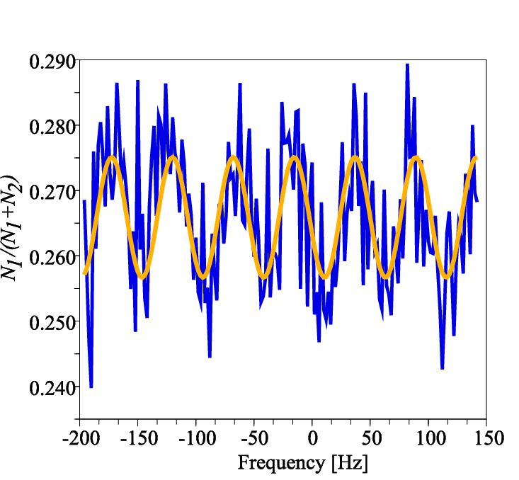
The Fig. 11 shows the proportion of atoms detected in the internal state $F=1$ as a function of the frequency difference between selection and measurement using the time sequence reported on Fig. 10.

The periodicity of the fringes (Fig. 11) is about $\delta_{\mathrm{sep}}=50\mathrm{~Hz}$ for the time sequence depicted on Fig. 10.

Quantitatively, $\delta_{\mathrm{sep}}$ can be compared with the periodicity of fringes of an interferometer without LMT Bloch pulses. With a delay of 5$\mathrm{~ms}$ between the two Ramsey pulses of the selection, the periodicity would have been 200$\mathrm{~Hz}$. Therefore with LMT pulses, the sensitivity of the interferometer is improved by about four.

We can define an effective time $T_{\mathrm{eff}}=1/\delta_{\mathrm{sep}}$, which is of about 20$\mathrm{~ms}$. Because the fringes spacing depends only on the separation of the two arms of the interferometer, the effective time $T_{\mathrm{eff}}$ can be viewed as the Ramsey time in a regular Ramsey-Bordé interferometer which leads to the same spatial separation of the two wave packets.

More rigorously, $T_{\mathrm{eff}}$ and the spatial separation $\left<X_{A}\right>-\left<X_{A}\right>$ of the two wave packets are linked through the following equation:

The dependence of $T_{\mathrm{eff}}$ with the duration of the selection sequence has been also investigated experimentally. The duration of the time-sequence of the interferometer is adjusted by changing ${T_{\mathrm{Ramsey}}}$ keeping the same $\pi/2$-Bloch-Bloch sequence. The variation of $T_{\mathrm{eff}}$ versus ${T_{\mathrm{Ramsey}}}$ is reported again on Fig. 12. There is an excellent agreement between experiment and calculations.

In the inset of the Fig. 12, we have also plotted the gain in resolution (ratio between the effective time and the real time) as a function of the duration of the selection. At the limit where ${T_{\mathrm{Ramsey}}}$ is long, the duration of the pulses can be neglected and the gain will be exactly $2N+1$, i.e. 5 for our parameters. At shorter times, this gain is smaller.

The experimental data fits well with the predicted time which is a strong evidence that the fringes observed on Fig. 11 are due to the LMT pulses.

Light shift in the interferometer are one of the main source of systematic effect. Furthermore they can induce a reduction of the contrast of interference.

The mean energy of atoms is indeed shifted when the lattice is switched on. This shift is not the same between the different bands and it depends on the intensity of the lattice. Our scheme (see Fig. 10) is on average symmetric: that is the time spent by atoms in a given energy band is equal for each arm of the interferometer. Consequently, there is no associated systematic shift if the intensity seen by atoms is constant. However, experimentally, this condition is never realized because of temporal fluctuations of the laser intensity and because of motion of the atoms through the spatial profile of the laser beam. In the first case, fluctuations of the intensity will be the same for each atom, leading to a phase noise in the interference pattern. In the second case, the light shift contribution will be averaged over all the atoms, leading to a reduction of the fringes contrast.

The light shift are implicitly included in the phase $\Phi_{\mathrm{Bloch}}$ obtained by integrating the Schrödinger equation. This phase depends on the intensity of the laser over time. For small variation of intensity, one could linearized the variation of the phase and compute the functional derivative of the phase with respect to the intensity:

In the experiment the intensity of the laser is modulate by an acousto-optic modulator. The intensity is therefore the product of the modulation ($M(t)$) due to the AOM and the intensity without modulation $I_{0}(t)$. If we assume that the modulation for the LMT pulse does not fluctuate ($\delta M(t)=0$), then the fluctuation of the phase is mainly due to fluctuations of $I_{0}(t)$ around its constant mean value $I_{0}$.

In the following instead of calculating $\frac{\delta\Phi}{\delta I(t)}$, we choose to calculate the functional derivative with respect to the normalized derivative of $I_{0}(t)$, $1/I_{0}\,\mathrm{d}I_{0}(t)/\mathrm{d}t$, that we denote by $g_{I}(t)$. We choose to use the derivative, because it is more convenient numerically and also lead to a dimensionless functional derivative. At first order, one can therefore write that:

In the following, $g_{I}$ is referred as the sensitivity function to the relative derivative of intensity.

Numerically, $g_{I}(t)$ is computed by looking to the variation of the phase $\Phi_{\mathrm{Bloch}}$ for a small change of the intensity $I_{0}(t^{\prime})$ for $t^{\prime}>t$ (Heaviside function). The temporal evolution of the function $g_{I}$ during the sequence described previously on Fig. 10 is reported on Fig. 13.

The inset is a zoom of $g_{I}$ at the beginning of the sequence. In the inset, the contributions to $g_{I}$ of each arm ($g_{I}^{A}$ and $g_{I}^{B}$) are plotted. In the experiment, atoms that are in excited band experience on average, the mean potential of the lattice, $U_{0}/2$, whereas atoms in the first band, are in dark region (blue detuned lattice) and less subjected to light shift.

The phases in the inset of Fig. 13 are calculated with eq. 6 in which the common light shift $U_{0}(t)/2$ is left out. This changes the values of $g_{I}^{A}$ and $g_{I}^{B}$ but not the value of $g_{I}$. Within this energy reference, an atom moving fast with respect to the lattice does not see a phase shift ($\left<\cos(2k\hat{x})\right>=0$) whereas an atom trapped into the lattice sees a phase shift ($\left<\cos(2k\hat{x})\right>\approx-1$). Therefore the main contribution to the phase shift originates from the lower band. Consequently, it explains why the initial increase of $g_{I}$ principally arises from the first band.

This phase shift is almost compensated by the other arm during the second LMT pulse. Indeed, the first two LMT pulses do not act in a symmetric way between the two arms because non-accelerated atoms are not in the same excited band during the first and second LMT pulses. During the first LMT pulse, non-accelerated atoms endure a small light shift (see the variation of $g_{I}^{B}$, around t=0.6$\mathrm{~ms}$ in the inset of Fig. 13, arrow labeled a). While during the second LMT pulse, non-accelerated atoms are moving too fast with respect to the lattice to see a light shift (see the plot of $g_{I}^{A}$ which remains constant during the second LMT, at $t$ around 1.2$\mathrm{~ms}$, arrow labeled b).

In the case of the interferometer with only four LMT pulses (see Fig. 9), the initial phase due to the first LMT pulse is compensated only at the end of the interferometer, after about 10$\mathrm{~ms}$, whereas in our scheme, 90% of this phase shift is compensate after 1$\mathrm{~ms}$. The sensitivity of our interferometer to a linear variation of the phase ($\int g_{I}(t)\mathrm{d}t$) is then reduced by a factor of 10 compared to an interferometer with four LMT pulses.

From the sensitivity function $g_{I}$, the reduction of the contrast due to the motion of atoms during the interferometer can be precisely calculated. For that, the phase shift accumulated along a trajectory must be calculated. At first order, it is expressed as

The contrast $C$ is given by $C=e^{-\Delta\phi^{2}/2}$ where $\Delta\phi$ is the variance of the phase $\phi$. $\Delta\phi$ is given by:

where $\sigma_{\dot{I}}$, which represents the relative variance of $\frac{\mathrm{d}I_{0}}{\mathrm{d}t}$ over the entire atomic cloud, is calculated with

To evaluate $\sigma_{\dot{I}}$ numerically, Gaussian distributions are used to described the position and the velocity of the atoms. Then $\sigma_{\dot{I}}$ can be expressed as:

in which $\sigma$ denotes the RMS value of the position of the atoms in one direction and $\sigma_{v}$ the RMS value of their velocity, $w_{L}$ represents the waist of the Gaussian laser beam. With ours experimental parameters ($w_{L}=2\mathrm{~mm}$, $\sigma=600\mathrm{~\mu m}$, $\sigma_{v}=2v_{r}$), the value of $\sigma_{\dot{I}}$ is around $5.9\mathrm{~s^{-1}}$.

For the eight LMT pulses scheme used in our experiment, we have calculated that: $\int g_{I}\mathrm{d}t\approx 48\times 10^{-3}\mathrm{~rad\cdot s}$. Therefore, the values of $\Delta\phi$ and $C$ are : $\Delta\phi=0.28\mathrm{~rad}$ and $C=96\%$.

With the four pulses scheme, those values become $\Delta\phi=2.8\mathrm{~rad}$ and $C=2\%$. This clearly shows that in our experiment, the eight LMT pulses scheme must be used to observe interferences.

We emphasize that there is a correlation between the velocity and the position of atoms because of the small time of flight before the beginning of the interferometer. This results in a biased intensity variation leading to a systematic effect in the interferometer. This effect can be canceled by inverting the order of the two LMT pulses for each beamsplitter because the sign of $g_{I}$ and consequently the one of $\phi$ is reversed.

The contrast of the fringes observed Fig. 11 is ten times smaller than the one without LMT pulses. This weak contrast can not be explain with light shifts. In the experiment, light shift is under control when the LMT pulses are used on both arms of the interferometer. Other sources contribute to this reduction. The main one arises from inhomogeneities in the initial momentum distribution of atoms and intensity of the laser. The maximum efficiency computed has been obtained for an atom with a defined velocity and a given laser intensity. But in our set-up, the initial velocity distribution is spread over about $0.5\,v_{r}$, consequently the effective efficiency for a LMT pulse is reduced from $98\%$ to $95\%$. Moreover, because of the initial size of the cloud and the finite waist of the laser, the variations of the intensity seen by atoms are in the order of $20\%$. As it can be easily see on Fig. 2, this effect pushes away the efficiency from the optimal configuration by few percents. The contribution of spontaneous emission of atoms trapped in the lattice is also non negligible. In our regular experiments with Bloch oscillations [18], atoms, located at the bottom of the lattice wells, are oscillating in the first band. As the potential of the lattice is blue detuned, the spontaneous emission is reduced, because the light intensity is minimal at the position of atoms [18]. Unfortunately, this demonstration does not apply to atoms in the excited bands. The estimated spontaneous emission rates of those atoms is around $4\%$.

All these effects added together reduce significantly the efficiency of each of the 8 LMT beamsplitter used in the interferometer and explain the reduction of contrast that we have observed. However, using a laser beam with a larger waist, a higher intensity (and a larger detuning) should allow us to reduce significantly these effects.

As mention previously, it is not possible to realize a larger momentum separation while keeping a good efficiency with the scheme of the LMT, in which constant acceleration is used (c.f. Fig 3).

To overcome this limitation, a process with different acceleration steps can be foreseen. The first step is identical to the one described earlier, with two Bloch oscillations. For the second one, the depth of the lattice is raised to enable a larger acceleration.

As explained previously, a long time and a relatively weak lattice are necessary to realize the first splitting with a good efficiency. For a given time, the optimal value of the amplitude of the lattice is a compromise between good adiabaticity of Bloch oscillations in the first band and a high Landau-Zener tunneling for the third band ($n=3$). However, this condition is less restricting when atoms are in a higher band ($n>3$). For those atoms, the Landau-Zener tunneling is higher so one can expect a better efficiency with the same duration or the same efficiency with a shorter duration. That is, a larger acceleration can be use to increase separation with a good efficiency.

The realization of a beam splitter with ten oscillations is presented on Fig. 14. The initial separation with two BOs is achieved in 130$\mathrm{~\mu s}$ while the second separation with eight BO is done in only 160$\mathrm{~\mu s}$. The maximal efficiency is calculated to be about $98\%$. This is very close to the efficiency with two BOs beamsplitter. The main losses arise from the initial splitting of two recoils. The additional losses come from the lack of adiabaticity during the change of the lattice intensity. As Bloch oscillations is a very efficient process, no significant losses arises from the additional recoils transferred after the first two oscillations. The main limitations will come from the reduction of contrast due to intensity fluctuations.

To estimate this limitation, the sensitivity function $g_{I}$, with ten BOs, is plotted on Fig. 15. It is significantly larger than the one with two BOs because of the increase of the depth of the lattice. The sensitivity to a linear variation of intensity $\int g_{I}\mathrm{d}t$ is about $95\times 10^{-3}\mathrm{~rad\cdot s}$. That is twice as much as the one for the interferometer with two BO (see section 3.1). This is the reason why the improved LMT was not implemented yet on our current apparatus (the visibility of fringes for the ”two BOs scheme” is already quite weak).

References

- (1) A. Wicht, J. Hensley, E. Sarajlic, S. Chu, Physica Scripta T102, 82 (2002)
- (2) M. Cadoret, E. de Mirandes, P. Cladé, S. Guellati-Khelifa, C. Schwob, F. Nez, L. Julien, F. Biraben, Phys. Rev. Lett. 101(23), 230801 (2008),
- (3) J.B. Fixler, G.T. Foster, J.M. McGuirk, M.A. Kasevich, Science 315, 74 (2007)
- (4) G. Lamporesi, A. Bertoldi, L. Cacciapuoti, M. Prevedelli, G.M. Tino, Physical Review Letters 100(5), 050801 (2008),
- (5) H. Müller, S. wey Chiow, S. Herrmann, S. Chu, K.Y. Chung, Physical Review Letters 100(3), 031101 (2008),
- (6) A. Peters, K. Chung, S. Chu, Nature 400, 849 (1999)
- (7) J. Le Gouët, T.E. Mehlstäubler, J. Kim, S. Merlet, A. Clairon, A. Landragin, F. Pereira Dos Santos, Applied Physics B: Lasers and Optics 92, 133 (2008),
- (8) H. Müller, S. wey Chiow, Q. Long, S. Herrmann, S. Chu, Phys. Rev. Lett. 100(18), 180405 (2008),
- (9) H. Müller, S. wey Chiow, S. Herrmann, S. Chu, Physical Review Letters 102(24), 240403 (2009),
- (10) T. Lévèque, A. Gauguet, F. Michaud, F.P.D. Santos, A. Landragin, Physical Review Letters 103(8), 080405 ( 4) (2009),
- (11) J.H. Denschlag, J.E. Simsarian, H. Häffner, C. McKenzie, A. Browaeys, D. Cho, K. Helmerson, S.L. Rolston, W.D. Phillips, Journal of Physics B Atomic Molecular Physics 35, 3095 (2002)
- (12) E. Peik, M.B. Dahan, I. Bouchoule, Y. Castin, C. Salomon, Phys. Rev. A 55, 2989 (1997)
- (13) P. Cladé, S. Guellati-Khélifa, F. Nez, F. Biraben, Physical Review Letters 102(24), 240402 (2009),
- (14) M.B. Dahan, E. Peik, J. Reichel, Y. Castin, C. Salomon, Phys. Rev. Lett. 76, 4508 (1996)
- (15) F. Bloch, Z. Phys 52, 555 (1929)
- (16) N. Ashcroft, N. Mermin, Solid State Physics (Brooks/Cole, 1976)
- (17) C. Zener, Proc. Soc. Lond. A 137, 696 (1932)
- (18) P. Cladé, E. de Mirandes, M. Cadoret, S. Guellati-Khélifa, C. Schwob, F. Nez, L. Julien, F. Biraben, Phys. Rev. A 74(5), 052109 (2006),
- (19) T. Hartmann, F. Keck, H.J. Korsch, S. Mossmann, New Journal of Physics 6(1), 2 (2004),
- (20) C. Bordé, Phys. Lett. A 140, 10 (1989)
- (21) P. Berman, Atom Interferometry (Academic Press, 1997)