Mass anomalous dimension in SU(2) with six fundamental fermions
Abstract
We simulate gauge theory with six massless fundamental Dirac fermions. We measure the running of the coupling and the mass in the Schrödinger Functional scheme. We observe very slow running of the coupling constant. We measure the mass anomalous dimension , and find it is between 0.135 and 1.03 in the range of couplings consistent with the existence of an IR fixed point.
CP3-Origins-2010-28
DAMTP-2010-51
1 Introduction
Phenomenologically viable models of technicolor can be built that are based on the existence of gauge theories with an infrared fixed point (IRFP) [1, 2]. The latter are asymptotically free theories where the dynamical effects of the fermion determinant induce a non-trivial zero of the beta functions at low energies, leading to scale-invariance at large distances. In particular the existence of a large mass anomalous dimension at the fixed point has been advocated as an important ingredient for model-building.
The phenomenology of strongly-interacting electroweak symmetry breaking has been summarized in several interesting reviews (see e.g. Ref. [3] for early results, and Refs. [4, 5] for the more recent developments.).
Several candidate theories have been singled out by analytical studies based on approximations of the full nonperturbative dynamics. A putative phase diagram which summarizes nicely the most appealing options was discussed in Ref. [6], see Ref. [7] for a review of recent results. These seminal results have triggered a number of numerical studies. Numerical simulations of theories defined on a spacetime lattice are indeed a privileged tool to study the nonperturbative dynamics of these theories from first principles. Current studies have focused on SU(2) with two adjoint Dirac fermions [10, 8, 9, 11, 12, 13, 14, 15, 16, 17, 18], SU(3) with 8,10,12 fermions in the fundamental representation [19, 20, 21, 22, 23, 24, 25, 26, 27, 28, 29, 30, 31, 32], SU(3) with two sextet fermions [33, 34, 35, 36, 28, 37, 38, 39, 40, 41], using a variety of methods. These studies have already revealed an interesting pattern of results about the phase diagram of strongly-interacting gauge theories, which can provide useful comparisons with (and hence guidance for) the analytical results.
In this work we focus on an SU(2) gauge theory with six flavors of Dirac fermions in the fundamental representation, which is supposed to be close to the lower boundary of the conformal window for the SU(2) color group. For example, the ladder approximation predicts that the conformal window begins at [6], the all-orders beta function conjecture predicts the lower boundary of the conformal window is at , which depends on the fixed point value of [42, 43], and metric confinement predicts the conformal window begins at [44]. This model is particularly relevant as it may be used for a practical realization of conformal technicolor theories [45, 46].
Using the Schrödinger Functional (SF) formulation of the theory [47, 48], we compute the running coupling and fermion mass as a function of the energy scale in the SF scheme, thereby deriving information on the beta function and the mass anomalous dimension. We find clear evidence that the running of the coupling is rather slow, and indeed compatible with the existence of a fixed point. As pointed out in previous studies [18], the identification of a fixed point by numerical techniques is intrinsically difficult: in the vicinity of the fixed point the coupling changes very slowly as a function of the scale; in order to detect a slow running, and to be able to identify precisely the location of the fixed point, great care must be exercised in taming the systematic errors that arise in numerical simulations. In particular we need to assess critically the systematic errors that are involved in our actual procedure, and their propagation in the analysis of the lattice data.
Contrary to the case of the gauge coupling, the running of the fermion mass does not slow down at the fixed point, and can be more easily identified by numerical methods. Results for the step-scaling function for the scale dependence of the renormalized mass, , yield a bound on the mass anomalous dimension at the fixed point, . Currently the main source of error in the determination of comes from the uncertainty in the value of the gauge coupling at the fixed point. First results for the anomalous dimension were obtained in Ref. [18] for the SU(2) gauge theory with adjoint fermions. Recently new results have been obtained for the SU(3) gauge theory with sextet fermions in Ref. [41].
The method used and the observables considered in this work are the same as the ones we implemented in Ref. [18]. They are briefly summarized for completeness in Section 2, together with the parameters of the runs that have been used for this analysis. The running of the coupling is encoded in the step scaling function ; our results for the latter are presented and critically discussed in Section 3. Finally the running of the mass is studied in Section 4; the data for the mass step scaling function compare favourably with the one-loop perturbative prediction, a feature that we also observed in our study of the SU(2) gauge theory with adjoint fermions. Even though we are unable determine whether a fixed point is present, our data are sufficiently precise to yield an upper bound on the value of the anomalous dimension throughout the range of couplings that we measure.
2 SF formulation
We measure the running coupling using the Schrödinger Functional method [47, 48]. We follow the same procedure as in Ref. [18] except for the change from two flavours of adjoint fermions to six flavours of fundamental fermions. Here we briefly describe the method; for a full description see Ref. [18].
The Schrödinger Functional coupling is defined on a hypercubic lattice of size . The boundary conditions are chosen to impose a constant background chromoelectric field, and depend on a parameter . The coupling constant is then defined as
| (1) |
with chosen such that to leading order in perturbation theory. This gives a non–perturbative definition of the coupling which depends only on and the lattice spacing . We then remove the lattice spacing dependence by taking the continuum limit.
We determine the mass anomalous dimension from the scale dependence of the pseudoscalar density renormalisation constant . This is defined as a ratio of correlation functions:
| (2) |
as in Ref. [18].
We use the Wilson plaquette gauge action, together with fundamental Wilson fermions, and an RHMC algorithm with 4 pseudofermions.
We run at , defined as the value of for which the PCAC mass vanishes. We measure for 5 values of for each on lattices and interpolate to find for each. We then extrapolate in to determine for the lattices.
In practice we achieve . At some values of and we have additional results at moderately small masses of , and we observe no mass-dependence within our statistical errors, confirming that any residual finite-mass errors are extremely small.
2.1 Lattice parameters
We have performed two sets of simulations in order to determine and . We use more values of (six instead of four) compared to our previous simulations to improve the quality of the continuum limit extrapolations, and increase the step scaling factor from to to improve the measurement of the slow running of the coupling.
To ensure our results are not affected by the presence of a bulk transition, we have measured the average plaquette for a range of values of and on lattices with SF boundary conditions. There is a clear jump in the plaquette at low , suggesting the presence of a bulk transition. However, this disappears around . Since the lowest we use for our measurements of and is , our results should not be affected by this transition.
The parameters of the runs are summarised in Table 1. The values of are obtained from the PCAC relation as described above.
| =6 | =8 | =12 | =16 | |||
|---|---|---|---|---|---|---|
| 2.0 | 0.151788 | 0.150970 | 0.150576 | 0.150491 | 0.150334 | 0.150252 |
| 2.2 | 0.147447 | 0.146939 | 0.146755 | 0.146782 | 0.146615 | 0.146565 |
| 2.5 | 0.143209 | 0.142825 | 0.142767 | 0.142811 | 0.142730 | 0.142716 |
| 3.0 | 0.138869 | 0.138684 | 0.138651 | 0.138562 | 0.138523 | 0.138493 |
| 3.5 | 0.136130 | 0.136143 | 0.136104 | 0.136103 | 0.136096 | 0.136091 |
| 4.0 | 0.134394 | 0.134350 | 0.134353 | 0.134339 | 0.134332 | 0.134327 |
| 5.0 | - | 0.132142 | 0.132142 | 0.132142 | 0.132142 | 0.132142 |
| 6.0 | 0.130753 | 0.130737 | 0.130748 | 0.130740 | 0.130739 | 0.130738 |
| 8.0 | 0.129131 | 0.129145 | 0.129167 | 0.129172 | 0.129177 | 0.129182 |
3 Results for the coupling
We have measured the coupling in the Schrödinger Functional scheme, , for a range of . Our results are shown in Table 2. We see immediately that the coupling is very similar for different at constant , so it runs slowly.
| =6 | =8 | =12 | =16 | |||
|---|---|---|---|---|---|---|
| 2.0 | 4.941(61) | 5.521(143) | 6.053(418) | 6.109(289) | 5.913(362) | 5.726(485) |
| 2.2 | 3.755(32) | 4.025(70) | 4.390(158) | 4.506(345) | 4.279(233) | 4.379(252) |
| 2.5 | 2.973(21) | 3.038(37) | 3.103(72) | 3.170(67) | 3.187(174) | 3.316(151) |
| 3.0 | 2.123(10) | 2.173(20) | 2.150(37) | 2.291(90) | 2.336(55) | 2.338(75) |
| 3.5 | 1.660(8) | 1.707(37) | 1.730(20) | 1.751(29) | 1.825(50) | 1.715(46) |
| 4.0 | 1.376(4) | 1.390(8) | 1.425(16) | 1.399(30) | 1.420(19) | 1.445(31) |
| 5.0 | - | 1.033(3) | 1.054(7) | 1.050(9) | 1.063(15) | 1.041(16) |
| 6.0 | 0.814(1) | 0.822(3) | 0.823(6) | 0.842(6) | 0.829(12) | 0.827(11) |
| 8.0 | 0.576(1) | 0.581(1) | 0.575(3) | 0.586(3) | 0.585(6) | 0.593(6) |
To analyse the running of the coupling we first define the lattice step-scaling function,
| (3) |
and its continuum limit:
| (4) |
where in both cases we will use only . We calculate from our data as follows:
We first discard the data since we have found it has large lattice artifacts. We then interpolate the remaining data quadratically in at each to find at . Then for each we interpolate in using the functional form [32, 18]
| (5) |
We choose the smallest which results in a such that the fit is not ruled out at a CL, and also use as the next best fit; this gives a 2-5 parameter fit in each case. The number of parameters we use for each and the for each fit are shown in Tables 3 and 4.
We now calculate using the fits from Eq. 5 for and . Finally we extrapolate to to obtain . Note that this extrapolation only makes sense when we are on the weak-coupling side of any IRFP.
We carry out a constant continuum extrapolation, using the data at the two values of closest to the continuum limit. We estimate the errors using a multistage bootstrapping procedure. The results for using the constant continuum extrapolation are plotted in Figure 1, where the statistical errors only are in black and the error from changing the number of fitting parameters are in grey. Our results are consistent with a fixed point in the region . They are also compatible with the possibility that there is no fixed point at all in the range of couplings we have measured. However, it is clear that is considerably below the 1-loop prediction at strong coupling.
We have also carried out a linear continuum extrapolation, using the data at the four values of closest to the continuum limit, but it is not as well constrained by our data. However, it is also below the 1-loop prediction at strong coupling, and has in the region . This is consistent with the presence of a fixed point in the region .
There is a large difference between the constant and continuum extrapolations, showing that the systematic error from the choice of continuum extrapolation is large. This means we cannot determine conclusively whether or not there is a fixed point in the range of couplings covered by our data.
| 8 | 10 | 12 | 14 | 15 | 16 | |||
| params | 3 | 4 | 4 | 4 | 3 | 2 | 2 | 2 |
| 1.92 | 0.54 | 1.24 | 0.48 | 1.66 | 1.54 | 1.88 | 1.36 | |
| 8 | 10 | 12 | 14 | 15 | 16 | |||
| params | 4 | 5 | 5 | 5 | 4 | 3 | 3 | 3 |
| 1.25 | 0.58 | 1.42 | 0.54 | 1.19 | 1.61 | 1.06 | 1.05 | |

In the vicinity of a fixed point at a coupling , the beta function is linear in the coupling,
| (6) |
where is a scheme-independent coefficient, which, as described in Ref. [49], yields further information on the physics of these theories. In terms of the step-scaling function , this gives:
| (7) |
We have estimated by fitting in the vicinity of the fixed point, and find , where the first error is statistical and the second is systematic, for those fits where we see a fixed point in the range of couplings covered by our data. This does not include the systematic error due to the choice of a constant rather than a linear continuum extrapolation. Better data would be needed to make the systematic errors on more robust.
4 Running mass
We have measured the pseudoscalar density renormalisation constant for a range of . Our results are shown in Table 5 and Figure 2. We see that decreases with increasing at constant , indicating a positive anomalous mass dimension, but the running appears to be slow.
| =6 | =8 | =12 | =16 | |||
|---|---|---|---|---|---|---|
| 2.00 | 0.26636(249) | 0.27219(306) | 0.27117(241) | 0.25956(527) | 0.24564(414) | 0.24130(578) |
| 2.20 | 0.33220(167) | 0.32060(216) | 0.30788(537) | 0.30929(137) | 0.29792(246) | 0.29198(215) |
| 2.50 | 0.37504(32) | 0.36203(49) | 0.35095(87) | 0.34672(73) | 0.34118(88) | 0.33255(162) |
| 3.00 | 0.40488(21) | 0.39186(31) | 0.38451(52) | 0.37955(50) | 0.37453(53) | 0.37170(56) |
| 3.50 | 0.42102(30) | 0.40981(82) | 0.40383(32) | 0.39832(43) | 0.39461(62) | 0.39241(93) |
| 4.00 | 0.43105(14) | 0.42192(21) | 0.41691(31) | 0.41256(34) | 0.40997(29) | 0.40746(36) |
| 6.00 | 0.45368(8) | 0.44908(12) | 0.44597(16) | 0.44417(10) | 0.44232(15) | 0.44045(20) |
| 8.00 | 0.46540(5) | 0.46229(7) | 0.46005(10) | 0.45822(7) | 0.45683(10) | 0.45575(9) |
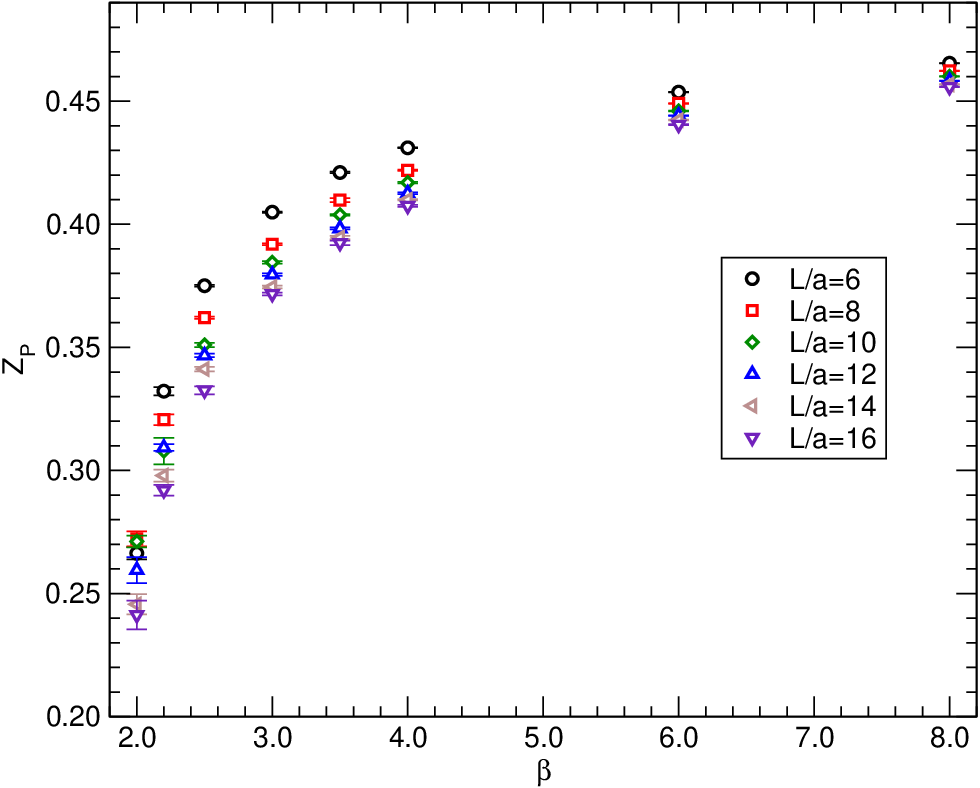
To extract we first define the lattice step-scaling function for the mass,
| (8) |
and its continuum limit
| (9) |
Again, we use only . To calculate , we proceed similarly as for . We first discard the data, and then interpolate quadratically in to find at . Then for each we interpolate in using the functional form [18]
| (10) |
We choose the smallest which results in an acceptable , as for the fits; this gives a 5-6 parameter fit in each case. We also use as a next-best fit to estimate the systematic errors from the choice of . The number of parameters we use for each and the for each fit are shown in Tables 6 and 7.
We can now calculate using Eq. 8 and the fits from Eq. 10, and finally extrapolate to the continuum limit to obtain . The errors are smaller than for the running coupling, so we are able to combine both constant and linear continuum extrapolations to control the systematic error from the choice of extrapolation. We estimate the errors using a multistage bootstrapping procedure.
We plot in Figure 3, where the statistical error is in black, and the systematic error arising both from the choice of the number of fit parameters and the continuum extrapolation is in grey. We also plot the 1-loop perturbative prediction for . Our results are close to the 1-loop prediction, with the running becoming a little faster at strong couplings.

In the vicinity of an IRFP, we can define an estimator given by
| (11) |
which is equal to the anomalous dimension at the fixed point [18], and deviates away from the fixed point as the anomalous dimension begins to run. We plot this estimator in Figure 4. Again the black error bars show the statistical errors, and the grey the systematic errors. We see that is small in most of the range of couplings that we measure. However, it becomes larger at our strongest couplings. Our data is consistent with it reaching values that are interesting for models of technicolor, although our error bars are large and it is also possible that it is as small as , our lower bound at , the smallest coupling at which a fixed point is consistent with our results using a constant continuum extrapolation. The highest value compatible with our data is at , the highest coupling at which we have results for all .
| 8 | 10 | 12 | 14 | 15 | 16 | |||
| params | 6 | 5 | 5 | 5 | 5 | 5 | 5 | 5 |
| 1.79 | 0.86 | 1.09 | 0.62 | 0.99 | 1.60 | 1.63 | 1.22 | |
| 8 | 10 | 12 | 14 | 15 | 16 | |||
| params | 7 | 6 | 6 | 6 | 6 | 6 | 6 | 6 |
| 2.09 | 0.46 | 1.03 | 0.43 | 1.18 | 0.93 | 1.32 | 1.47 | |

5 Conclusions
In this work we have calculated the running of the Schrödinger Functional coupling and the mass in the continuum limit of lattice gauge theory with six flavours of fundamental fermions, over a wide range of couplings up to .
Our results for the running of the coupling have relatively large errors. This is due to the difficulty of measuring the small difference in the coupling between two nearby scales, a problem that becomes particularly acute as we approach a possible fixed point where the difference falls. We observe that the running of the coupling is slower than the (already slow) one-loop perturbative prediction. Our results using a constant continuum extrapolation are consistent with the presence of a fixed point above , but it is also possible that there is no fixed point in the range of couplings we have measured. There is an additional uncertainty arising from the choice of continuum extrapolation.
Our results for the running of the mass are clearer. We find the anomalous dimension is small throughout most of the range of couplings we measure, but it becomes larger for our strongest couplings, with a possibility that it reaches values around 1. If true, this would be very interesting for technicolor models.
The value of at the fixed point can be predicted using the all-orders beta function conjecture [42]. This gives an exact prediction in terms of group-theoretical factors only. If the present theory is inside the conformal window, the prediction is , which lies outside the range measured in this study. Unfortunately, given the uncertainty on the existence of the fixed point, any conclusion on the validity of the all-order beta function conjecture is speculative at present.
The accuracy of our results would be improved in particular by using larger lattices, which would give a larger range of for the continuum extrapolations. This would help to clarify the existence and location of the fixed point, and to reduce the errors on the anomalous dimension. Calculations to improve the statistics and use larger lattice sizes are ongoing.
Acknowledgements
This work was performed using the Darwin Supercomputer of the University of Cambridge High Performance Computing Service (http://www.hpc.cam.ac.uk/), provided by Dell Inc. using Strategic Research Infrastructure Funding from the Higher Education Funding Council for England; computing resources funded by the University of Oxford and EPSRC; and the Horseshoe5 cluster at the supercomputing facility at the University of Southern Denmark (SDU) funded by a grant of the Danish Centre for Scientific Computing for the project ‘Origin of Mass’ 2008/2009. LDD wishes to thank the Aspen Center for Physics where part of this work has been carried out. LDD is supported by an STFC Advanced Fellowship.
References
- [1] William E. Caswell. Asymptotic Behavior of Nonabelian Gauge Theories to Two Loop Order. Phys. Rev. Lett., 33:244, 1974.
- [2] Tom Banks and A. Zaks. On the phase structure of vector-like gauge theories with massless fermions. Nucl. Phys., B196:189, 1982.
- [3] Christopher T. Hill and Elizabeth H. Simmons. Strong dynamics and electroweak symmetry breaking. Phys. Rept., 381:235–402, 2003.
- [4] Francesco Sannino. Conformal Dynamics for TeV Physics and Cosmology. 2009.
- [5] Maurizio Piai. Lectures on walking technicolor, holography and gauge/gravity dualities. 2010.
- [6] Dennis D. Dietrich and Francesco Sannino. Conformal window of su(n) gauge theories with fermions in higher dimensional representations. Phys. Rev., D75:085018, 2007.
- [7] Francesco Sannino. Dynamical Stabilization of the Fermi Scale: Phase Diagram of Strongly Coupled Theories for (Minimal) Walking Technicolor and Unparticles. 2008.
- [8] Luigi Del Debbio, Mads T. Frandsen, Haralambos Panagopoulos, and Francesco Sannino. Higher representations on the lattice: perturbative studies. JHEP, 06:007, 2008.
- [9] Luigi Del Debbio, Agostino Patella, and Claudio Pica. Higher representations on the lattice: numerical simulations. SU(2) with adjoint fermions. 2008.
- [10] Simon Catterall and Francesco Sannino. Minimal walking on the lattice. Phys. Rev., D76:034504, 2007.
- [11] Simon Catterall, Joel Giedt, Francesco Sannino, and Joe Schneible. Phase diagram of SU(2) with 2 flavors of dynamical adjoint quarks. JHEP, 11:009, 2008.
- [12] Luigi Del Debbio, Agostino Patella, and Claudio Pica. Fermions in higher representations. Some results about SU(2) with adjoint fermions. 2008.
- [13] Ari J. Hietanen, Jarno Rantaharju, Kari Rummukainen, and Kimmo Tuominen. Spectrum of SU(2) lattice gauge theory with two adjoint Dirac flavours. JHEP, 05:025, 2009.
- [14] Ari Hietanen, Jarno Rantaharju, Kari Rummukainen, and Kimmo Tuominen. Spectrum of SU(2) gauge theory with two fermions in the adjoint representation. PoS, LATTICE2008:065, 2008.
- [15] L. Del Debbio, B. Lucini, A. Patella, C. Pica, and A. Rago. Conformal vs confining scenario in SU(2) with adjoint fermions. Phys. Rev., D80:074507, 2009.
- [16] C. Pica, L. Del Debbio, B. Lucini, A. Patella, and A. Rago. Technicolor on the Lattice. 2009.
- [17] Ari J. Hietanen, Kari Rummukainen, and Kimmo Tuominen. Evolution of the coupling constant in SU(2) lattice gauge theory with two adjoint fermions. Phys. Rev., D80:094504, 2009.
- [18] Francis Bursa, Luigi Del Debbio, Liam Keegan, Claudio Pica, and Thomas Pickup. Mass anomalous dimension in SU(2) with two adjoint fermions. Phys. Rev., D81:014505, 2010.
- [19] Zoltan Fodor, Kieran Holland, Julius Kuti, Daniel Nogradi, and Chris Schroeder. Probing technicolor theories with staggered fermions. PoS, LATTICE2008:066, 2008.
- [20] Albert Deuzeman, Maria Paola Lombardo, and Elisabetta Pallante. The physics of eight flavours. Phys. Lett., B670:41–48, 2008.
- [21] Albert Deuzeman, Maria Paola Lombardo, and Elisabetta Pallante. The physics of eight flavours. PoS, LATTICE2008:060, 2008.
- [22] Albert Deuzeman, Elisabetta Pallante, Maria Paola Lombardo, and E. Pallante. Hunting for the Conformal Window. PoS, LATTICE2008:056, 2008.
- [23] A. Deuzeman, M. P. Lombardo, and E. Pallante. Evidence for a conformal phase in SU(N) gauge theories. 2009.
- [24] Albert Deuzeman, Maria Paola Lombardo, and Elisabetta Pallante. Traces of a fixed point: Unravelling the phase diagram at large Nf. 2009.
- [25] Zoltan Fodor, Kieran Holland, Julius Kuti, Daniel Nogradi, and Chris Schroeder. Calculating the running coupling in strong electroweak models. 2009.
- [26] Zoltan Fodor, Kieran Holland, Julius Kuti, Daniel Nogradi, and Chris Schroeder. Chiral symmetry breaking in nearly conformal gauge theories. 2009.
- [27] Xiao-Yong Jin and Robert D. Mawhinney. Lattice QCD with Eight Degenerate Quark Flavors. PoS, LATTICE2008:059, 2008.
- [28] Zoltan Fodor, Kieran Holland, Julius Kuti, Daniel Nogradi, and Chris Schroeder. Topology and higher dimensional representations. JHEP, 08:084, 2009.
- [29] Zoltan Fodor, Kieran Holland, Julius Kuti, Daniel Nogradi, and Chris Schroeder. Nearly conformal gauge theories in finite volume. Phys. Lett., B681:353–361, 2009.
- [30] Thomas Appelquist, George T. Fleming, and Ethan T. Neil. Lattice Study of the Conformal Window in QCD-like Theories. Phys. Rev. Lett., 100:171607, 2008.
- [31] George T. Fleming. Strong Interactions for the LHC. PoS, LATTICE2008:021, 2008.
- [32] Thomas Appelquist, George T. Fleming, and Ethan T. Neil. Lattice Study of Conformal Behavior in SU(3) Yang-Mills Theories. Phys. Rev., D79:076010, 2009.
- [33] Thomas DeGrand, Yigal Shamir, and Benjamin Svetitsky. Exploring the phase diagram of sextet QCD. PoS, LATTICE2008:063, 2008.
- [34] Thomas DeGrand, Yigal Shamir, and Benjamin Svetitsky. Phase structure of SU(3) gauge theory with two flavors of symmetric-representation fermions. Phys. Rev., D79:034501, 2009.
- [35] Zoltan Fodor, Kieran Holland, Julius Kuti, Daniel Nogradi, and Chris Schroeder. Nearly conformal electroweak sector with chiral fermions. PoS, LATTICE2008:058, 2008.
- [36] Zoltan Fodor, Kieran Holland, Julius Kuti, Daniel Nogradi, and Chris Schroeder. Chiral properties of SU(3) sextet fermions. JHEP, 11:103, 2009.
- [37] Thomas DeGrand. Volume scaling of Dirac eigenvalues in SU(3) lattice gauge theory with color sextet fermions. 2009.
- [38] Thomas DeGrand. Finite-size scaling tests for SU(3) lattice gauge theory with color sextet fermions. Phys. Rev., D80:114507, 2009.
- [39] Benjamin Svetitsky, Yigal Shamir, and Thomas DeGrand. Nonperturbative infrared fixed point in sextet QCD. PoS, LATTICE2008:062, 2008.
- [40] Yigal Shamir, Benjamin Svetitsky, and Thomas DeGrand. Zero of the discrete beta function in SU(3) lattice gauge theory with color sextet fermions. 2008.
- [41] Thomas DeGrand, Yigal Shamir, and Benjamin Svetitsky. Running coupling and mass anomalous dimension of SU(3) gauge theory with two flavors of symmetric-representation fermions. 2010.
- [42] Thomas A. Ryttov and Francesco Sannino. Supersymmetry Inspired QCD Beta Function. Phys. Rev., D78:065001, 2008.
- [43] Francesco Sannino. Conformal Windows of SP(2N) and SO(N) Gauge Theories. Phys. Rev., D79:096007, 2009.
- [44] Mads T. Frandsen, Thomas Pickup and Michael Teper. Delineating the conformal window. 2010.
- [45] Markus A. Luty and Takemichi Okui. Conformal technicolor. JHEP, 09:070, 2006.
- [46] Hidenori S. Fukano and Francesco Sannino. Conformal Window of Gauge Theories with Four-Fermion Interactions and Ideal Walking. 2010.
- [47] Martin Luscher, Peter Weisz and Ulli Wolff. A Numerical method to compute the running coupling in asymptotically free theories Nucl. Phys., B359:221–243, 1991.
- [48] Martin Luscher, Rajamani Narayanan, Peter Weisz, and Ulli Wolff. The Schrodinger functional: A Renormalizable probe for nonAbelian gauge theories. Nucl. Phys., B384:168–228, 1992.
- [49] Einan Gardi and Georges Grunberg. The conformal window in QCD and supersymmetric QCD. JHEP, 03:024, 1999.