跳到论文正文
W Papers独立论文阅读器 arXiv:1007.3052 论文正文 计算阅读时间 · 0%
引用这篇论文根据当前论文元数据生成,正式投稿前建议核对。


License: arXiv.org perpetual non-exclusive license
arXiv:1007.3052v2 [math.AP] 10 Aug 2010

On the Sacks-Uhlenbeck flow of Riemannian surfaces

Min-Chun Hong and Hao Yin Address: Min-Chun Hong, Department of Mathematics, The University of Queensland
Brisbane, QLD 4072, Australia
Email address: hong@maths.uq.edu.au Address: Hao Yin, Department of Mathematics, The University of Queensland
Brisbane, QLD 4072, Australia and Department of Mathematics, Shanghai Jiaotong University, Shanghai, China
Email address: haoyin@sjtu.edu.cn
Abstract.

In this paper, we study an α\alpha-flow for the Sacks-Uhlenbeck functional on Riemannian surfaces and prove that the limiting map by the α\alpha-flows is a weak solution to the harmonic map flow. By an application of the α\alpha-flow, we present a simple proof of an energy identity of a minimizing sequence in each homotopy class.

Key words and phrases: 
harmonic map flow, Sacks-Uhlenbeck functional
1991 Mathematics Subject Classification
AMS 58E20, 35K45
\markleft

1. Introduction

Suppose that MM is a Riemannian manifold and NN is a closed manifold embedded in ℝk\mathbb{R}^{k}. A critical point uu of the Dirichlet energy

E⁡(u)=∫M|∇u|2​𝑑vE(u)=\int_{M}\left|\nabla u\right|^{2}dv

is called a harmonic map.

Harmonic maps between Riemannian manifolds can be thought of as a natural generalization of geodesics, minimal surfaces and harmonic functions. A fundamental question is: Given a smooth map u0u_{0} from MM to NN, does there exist a smooth harmonic map representative in the homotopy class of u0u_{0}? In a pioneering work [7], Eells and Sampson introduced the harmonic map flow and used it to deform an initial map to a harmonic map in the same homotopic class if the sectional curvature of NN is non-positive. In general, one cannot expect to have the existence of smooth harmonic maps into general target manifolds due to the fact that singularities do occur. From now on, we assume that MM is a closed Riemannian surface, hence E⁡(u)E(u) is conformally invariant. Under certain topological conditions of NN, the existence of minimizing harmonic maps in a homotopy class was proved by Lemaire [11] and Schoen-Yau [21]. In a well-known paper [18], Sacks and Uhlenbeck proposed a family of the perturbed functional

Eα​(u)=∫M(1+|∇u|2)α​𝑑vE_{\alpha}(u)=\int_{M}(1+\left|\nabla u\right|^{2})^{\alpha}dv

for α>1\alpha>1. The advantage of the perturbed functional is that EαE_{\alpha} satisfies the Palais-Smale condition and therefore it is easy to obtain critical points of EαE_{\alpha} by either minimizing energy functional or Morse theory. When α→1\alpha\to 1, the limiting map of critical points of EαE_{\alpha} is a harmonic map and a bubbling phenomenon occurs.

On the other hand, Struwe [22] proved the global existence of the weak solution to the harmonic map flow and that the solution to the flow converges to a harmonic map as t→∞t\to\infty. Chang, Ding and Ye [2] constructed an example that the harmonic map flow blowups at finite time, so in general the limit harmonic map by the flow may not be in the same homotopy class of the initial map.

In this paper, we study an α\alpha-flow for the perturbed energy EαE_{\alpha} in the same homotopy class of the initial map. More precisely, we consider the following evolution problem:

(1.1) ∂tu=△M​u+(α−1)​∇|∇u|2⋅∇u1+|∇u|2+A⁡(u)​(∇u,∇u)\partial_{t}u=\triangle_{M}u+(\alpha-1)\frac{\nabla\left|\nabla u\right|^{2}\cdot\nabla u}{1+\left|\nabla u\right|^{2}}+A(u)(\nabla u,\nabla u)

with u⁡(x,0)=u0u(x,0)=u_{0}, where △M\triangle_{M} is the Laplacian operator with respect to the Riemannian metric of MM and AA is the second fundamental form of NN. We call (1.1) the Sacks-Uhlenbeck flow (or α\alpha-flow). We would like to point out that the α\alpha-flow is not the standard gradient flow, but the flow has some analytic advantage.

At first, we have

Theorem 1.1.

For a given smooth map u0:M→Nu_{0}:M\to N, there exists a unique global smooth solution uα​(x,t)u_{\alpha}(x,t) to the evolution problem (1.1) in M×[0,∞)M\times[0,\infty). Moreover, for any ti→∞t_{i}\to\infty, uα​(⋅,ti)u_{\alpha}(\cdot,t_{i}) converges smoothly to a limit map uαu_{\alpha}, which is a critical point of the Sacks-Uhlenbeck functional for α−1\alpha-1 sufficiently small.

For each α>1\alpha>1, let uα​(x,t)u_{\alpha}(x,t) be the global smooth solution to (1.1) in the same homotopy class with the initial map u0u_{0} from MM to NN. There is a nature problem to study the limit behaviour of the solution uα​(x,t)u_{\alpha}(x,t) as α→1\alpha\to 1 as one in [18]. Thus, we prove

Theorem 1.2.

(i) As α→1\alpha\to 1, the solution uαu_{\alpha} converges smoothly to uu on M×[0,∞)∖ΣM\times[0,\infty)\setminus\Sigma, where the concentration set Σ\Sigma is a closed set defined by

Σ=⋂0<R<RM{z∈M×[0,∞)|lim infα→1ΨRα(uα,z)≥ε0}\Sigma=\bigcap_{0<R<R_{M}}\left\{z\in M\times[0,\infty)|\quad\liminf_{\alpha\to 1}\Psi^{\alpha}_{R}(u_{\alpha},z)\geq\varepsilon_{0}\right\}

for some ε0\varepsilon_{0} to be determined. For the precise definition of ΨRα\Psi_{R}^{\alpha}, see Section 3.

(ii) For any two positive t1t_{1} and t2t_{2}, 𝒫2​(Σ∩(M×[t1,t2]))\mathcal{P}^{2}(\Sigma\cap(M\times[t_{1},t_{2}])) is finite, where 𝒫2\mathcal{P}^{2} denotes the 22-dimensional parabolic Hausdorff measure. Moreover, for any t∈(0,+∞)t\in(0,+\infty), Σt=Σ∩(M×{t})\Sigma_{t}=\Sigma\cap(M\times\{t\}) consists of at most finitely many points.

(iii) uu is a weak solution to the harmonic map flow.

In fact, this result is similar to the one by the Ginzburg-Landau flow approximation. In [4], Chen and Struwe used the Ginzburg-Landau flow approximation to construct a global weak solution of the harmonic map flow for any dimension larger than two. Further results obtained by the Ginzburg-Landau flow were discussed by Lin and Wang in [15]. The method by the Ginzburg-Landau flow is very powerful to show the global existence and partial regularity of a weak solution to the harmonic map flow, but it seems that the flow loses control on the topological quantity of maps. The advantage of the Sacks-Uhlenbeck flow approximation is that the solution uαu_{\alpha} remains in the same homotopy class of u0u_{0}, therefore it seems that the Sacks-Uhlenbeck flow provides a nice geometric picture and can be used to have some geometric applications (see Theorem 1.4 below).

Without the assumption of the energy inequality, weak solutions to the heat flow for harmonic maps may not always be unique (see [1] and [24]), so it is very interesting whether the limiting solution uu by the Sacks-Uhlenbeck flow is the global weak solution u^\hat{u} constructed by Struwe in [22]. Although we do not have a complete answer to the question, we can compare some property of uu with the one of u^\hat{u} in the following:

Theorem 1.3.

(i) The first concentration time for uαu_{\alpha} as α→1\alpha\to 1; i.e.

T=inf(x,t)∈ΣtT=\inf_{(x,t)\in\Sigma}t

is the same as the first singular time of the Struwe’s weak solution. Hence, uαu_{\alpha} converges smoothly to the Struwe’s solution in M×[0,T)M\times[0,T).

(ii) Consider the following two limits of measures

|∇u^​(⋅,t)|2​d​v→|∇u^​(⋅,T)|2​d​v+∑i=1k^m^i​δp^ias ​t→T|\nabla\hat{u}(\cdot,t)|^{2}dv\to|\nabla\hat{u}(\cdot,T)|^{2}dv+\sum_{i=1}^{\hat{k}}\hat{m}_{i}\delta_{\hat{p}_{i}}\quad\mbox{as }t\to T

and

(1+|∇uα​(T,α)|2)α​d​v→(1+|∇u​(⋅,T)|2)​d​v+∑i=1kmi​δpias ​α→1.(1+|\nabla u_{\alpha}(T,\alpha)|^{2})^{\alpha}dv\to(1+|\nabla u(\cdot,T)|^{2})\,dv+\sum_{i=1}^{k}m_{i}\delta_{p_{i}}\quad\mbox{as }\alpha\to 1.

Then k=k^k=\hat{k}, pi=p^ip_{i}=\hat{p}_{i} and m^i≥mi\hat{m}_{i}\geq m_{i}.

Moreover, we can obtain more refined information about the singularity points of uu and Σ\Sigma (see Lemma 3.3).

In the final part of this paper, we apply the α−\alpha-flow to study a minimizing sequence in a given homotopy class. Let uiu_{i} be a sequence of smooth maps minimizing E⁡(u)=∫M|∇u|2​𝑑vE(u)=\int_{M}\left|\nabla u\right|^{2}dv in a fixed homotopy class of maps. Since uiu_{i} is bounded in W1,2W^{1,2}, there is a weak limit uu in W1,2​(M,N)W^{1,2}(M,N). In general, uu may not be in the same homotopy class, but we can show:

Theorem 1.4.

Let uu be the weak limit of above minimizing sequence {ui}\{u_{i}\}. Then it is a harmonic map from MM to NN and there exist harmonic maps ωk:S2→N\omega_{k}:S^{2}\to N with k=1,⋯,lk=1,\cdots,l such that

(1.2) limi→∞E⁡(ui)=E⁡(u)+∑k=1lE⁡(ωk).\lim_{i\to\infty}E(u_{i})=E(u)+\sum_{k=1}^{l}E(\omega_{k}).

Moreover, if π2​(N)\pi_{2}(N) is trivial, then uiu_{i} converges strongly to uu in W1,2​(M,N)W^{1,2}(M,N) and uu is a minimizer in the homotopy class of uiu_{i}.

The last part of this theorem can be compared with Theorem 5.1 of [18], where under the same assumption that π2​(N)\pi_{2}(N) is trivial, the existence of a minimizer in each homotopy class is proved (see also [21] and [11]). We improve the result a little by obtaining that every smooth minimizing sequence converges to such a minimizer. In the proof, we use the α−\alpha-flow to modify the original minimizing sequence and study the blow-up of the new sequence as Theorem 5.1 in [18]. The energy identity of minimizers of the Sacks-Uhlenbeck functional was implicitly established by Chen and Tian in [3]. Our proof for the energy identity is different from one in [3]. Although the result of Theorem 1.4 may be regarded as a consequence of the theory developed by Duzaar and Kuwert [6], the advantage is that we can avoid to use the concept “weak homotopy class” of maps in the Sobolev space W1,2​(M,N)W^{1,2}(M,N), which is formulated by big machinery. Finally, we would like to mention that the related energy identity of critical points of the Sacks-Uhlenbeck functionals was recently discussed by Li and Wang [13] and by Lamm [10].

Remark 1.5.

After we finished a first version of this paper, Yuxiang Li informed us that in [14] they used a similar idea to show the energy identify for a sequence of minimizers of EαE_{\alpha} when α→1\alpha\to 1. In fact, while Li and Wang in [14] used a reduction procedure of Ding and Tian [5], we use the bubble tree construction of Parker in [17] and Lemma 5.4 to find the connecting geodesics, so our approach is different.

The paper is organized as follows. In Section 2, we prove Theorem 1.1. In Section 3, we give a proof of Theorem 1.2. In Section 4, we complete a proof of Theorem 1.3 except for the energy identity, which is proved in Section 5.

2. global existence and convergence of α−\alpha-flow

This section is devoted to the proof of Theorem 1.1. In local coordinates g=(gi​j)g=(g_{ij}), the α\alpha-flow can be written as

∂tu=1|g|​∂∂xi​(|g|​gi​j​∂u∂xj)+(α−1)​gi​j​∂∂xi​|∇u|2​∂u∂xj1+|∇u|2+A⁡(u)​(∇u,∇u).\partial_{t}u=\frac{1}{\sqrt{\left|g\right|}}\frac{\partial}{\partial x_{i}}\left(\sqrt{\left|g\right|}g^{ij}\frac{\partial u}{\partial x_{j}}\right)+(\alpha-1)\frac{g^{ij}\frac{\partial}{\partial x_{i}}\left|\nabla u\right|^{2}\frac{\partial u}{\partial x_{j}}}{1+\left|\nabla u\right|^{2}}+A(u)(\nabla u,\nabla u).

This system is a nonlinear parabolic system. For a smooth initial value u0u_{0}, the local existence of the system can be shown (see below appendix for details in Section 6); i.e., there exists T>0T>0 and a smooth solution u⁡(x,t)u(x,t) defined on [0,T)[0,T). The proof of Theorem 1.1 follows if one can establish CkC^{k} uniform estimates of u⁡(x,t)u(x,t) independent of TT for any t∈[0,T)t\in[0,T).

The first observation is that

Lemma 2.1.

If u⁡(x,t)u(x,t) is a solution to the α−\alpha-flow, then Eα​(u​(⋅,t))E_{\alpha}(u(\cdot,t)) decreases in tt.

Proof.

Multiply (1.1) by (1+|∇u|2)α−1​∂tu(1+\left|\nabla u\right|^{2})^{\alpha-1}\partial_{t}u and integrate by parts. ∎

The next lemma is a local version of the energy inequality.

Lemma 2.2.

Let uu be a solution to the α−\alpha-flow. Then

(2.1) ∫BR​(x)(1+|∇u​(⋅,t2)|2)α​𝑑v≤∫B2​R​(x)(1+|∇u​(⋅,t1)|2)α​𝑑v+C​t2−t1R2​E0\int_{B_{R}(x)}(1+\left|\nabla u(\cdot,t_{2})\right|^{2})^{\alpha}dv\leq\int_{B_{2R}(x)}(1+\left|\nabla u(\cdot,t_{1})\right|^{2})^{\alpha}dv+C\frac{t_{2}-t_{1}}{R^{2}}E_{0}

for t1<t2t_{1}<t_{2}. Here E0E_{0} is some upper-bound of the overall energy.

Proof.

Let φ\varphi be a cut-off function supported in BR​(x)B_{R}(x) and φ≡1\varphi\equiv 1 on BR/2​(x)B_{R/2}(x). Multiplying the equation (1.1) by (1+|∇u|2)α−1​∂tu​φ2(1+\left|\nabla u\right|^{2})^{\alpha-1}\partial_{t}u\varphi^{2}, we obtain

∫M(1+|∇u|2)α−1​|∂tu|2​φ2​𝑑v\displaystyle\int_{M}(1+\left|\nabla u\right|^{2})^{\alpha-1}\left|\partial_{t}u\right|^{2}\varphi^{2}dv
=\displaystyle= −∫M(1+|∇u|2)α−1∇u∇∂u∂tφ2dv−∫M(1+|∇u|2)α−1∇u∂u∂t2φ∇φdv\displaystyle-\int_{M}(1+\left|\nabla u\right|^{2})^{\alpha-1}\nabla u\nabla\frac{\partial u}{\partial t}\varphi^{2}dv-\int_{M}(1+\left|\nabla u\right|^{2})^{\alpha-1}\nabla u\frac{\partial u}{\partial t}2\varphi\nabla\varphi dv
≤\displaystyle\leq −1αdd​t∫M(1+|∇u|2)αφ2dv+12∫M(1+|∇u|2)α−1|∂tu|2φ2dv\displaystyle-\frac{1}{\alpha}\frac{d}{dt}\int_{M}(1+\left|\nabla u\right|^{2})^{\alpha}\varphi^{2}dv+\frac{1}{2}\int_{M}(1+\left|\nabla u\right|^{2})^{\alpha-1}\left|\partial_{t}u\right|^{2}\varphi^{2}dv
+∫B2​R​(x)(1+|∇u|2)α−1|∇u|2CR2dv.\displaystyle+\int_{B_{2R(x)}}(1+\left|\nabla u\right|^{2})^{\alpha-1}\left|\nabla u\right|^{2}\frac{C}{R^{2}}dv.

Hence,

∫BR​(x)(1+|∇u​(⋅,t2)|2)α​𝑑v≤∫B2​R​(x)(1+|∇u​(⋅,t1)|2)α​𝑑v+C​t2−t1R2​E0.\int_{B_{R}(x)}(1+\left|\nabla u(\cdot,t_{2})\right|^{2})^{\alpha}dv\leq\int_{B_{2R}(x)}(1+\left|\nabla u(\cdot,t_{1})\right|^{2})^{\alpha}dv+C\frac{t_{2}-t_{1}}{R^{2}}E_{0}.

∎

The second key for the proof of Theorem 1.1 is to derive a Bochner type formula. We consider a scaled version of (1.1) for some r>0r>0,

(2.2) (r2+|∇u|2)α−1∂tu=div((r2+|∇u|2)α−1∇u)+(r2+|∇u|2)α−1A(u)(∇u,∇u).(r^{2}+\left|\nabla u\right|^{2})^{\alpha-1}\partial_{t}u=\mbox{div}\left((r^{2}+\left|\nabla u\right|^{2})^{\alpha-1}\nabla u\right)+(r^{2}+\left|\nabla u\right|^{2})^{\alpha-1}A(u)(\nabla u,\nabla u).

Locally, we choose an orthonormal frame {e1,e2}\{e_{1},e_{2}\}. We use ∇i\nabla_{i} for the first covariant derivative with respect to eie_{i}. We denote by uj​iu_{ji} the second covariant derivatives of uu and so on. Of course, we assume summation convention for repeated index. Then

Lemma 2.3.

Let u⁡(x,t)u(x,t) be a smooth solution to the scaled α−\alpha-flow (2.2). If α−1\alpha-1 is small, then the following Bochner type formula is true:

(2.3) ∂∂t​e​(u)−∇i((δi​j+2​(α−1)​uiβ​ujβr2+|∇u|2)​∇je​(u))≤C​e​(u)​(e⁡(u)+1),\frac{\partial}{\partial t}e(u)-\nabla_{i}\left((\delta_{ij}+2(\alpha-1)\frac{u^{\beta}_{i}u^{\beta}_{j}}{r^{2}+\left|\nabla u\right|^{2}})\nabla_{j}e(u)\right)\leq Ce(u)(e(u)+1),

where e⁡(u):=|∇u|2e(u):=\left|\nabla u\right|^{2}.

Proof.

The proof is by computation. In the following proofs, we assume α−1\alpha-1 is small whenever necessary. In a local frame, we have

∇je​(u)=2​ukγ​uk​jγ,|∇2u|2=∑k,i,γ|uk​iγ|2\nabla_{j}e(u)=2u^{\gamma}_{k}u^{\gamma}_{kj},\quad|\nabla^{2}u|^{2}=\sum_{k,i,\gamma}\left|u^{\gamma}_{ki}\right|^{2}

Then we have

∇i((δi​j+2​(α−1)​uiβ​ujβr2+|∇u|2)​∇je​(u))\displaystyle\nabla_{i}\left((\delta_{ij}+2(\alpha-1)\frac{u^{\beta}_{i}u^{\beta}_{j}}{r^{2}+\left|\nabla u\right|^{2}})\nabla_{j}e(u)\right)
=\displaystyle= 2​∇i(ukγ​uk​iγ+2​(α−1)​uiβ​ujβ​ukγ​uk​jγr2+|∇u|2)\displaystyle 2\nabla_{i}\left(u^{\gamma}_{k}u^{\gamma}_{ki}+2(\alpha-1)\frac{u^{\beta}_{i}u^{\beta}_{j}u^{\gamma}_{k}u^{\gamma}_{kj}}{r^{2}+\left|\nabla u\right|^{2}}\right)
≥\displaystyle\geq 2​|∇2u|2+2​ukγ​ui​i​kγ+4​(α−1)​∇i(uiγ​ukγ​ujβ​uk​jβr2+|∇u|2)−C​e​(u)\displaystyle 2|\nabla^{2}u|^{2}+2u^{\gamma}_{k}u^{\gamma}_{iik}+4(\alpha-1)\nabla_{i}\left(\frac{u^{\gamma}_{i}u^{\gamma}_{k}u^{\beta}_{j}u^{\beta}_{kj}}{r^{2}+\left|\nabla u\right|^{2}}\right)-Ce(u)
≥\displaystyle\geq 32​|∇2u|2+2​ukγ​ui​i​kγ+4​(α−1)​uiγ​ukγ​ujβ​uk​j​iβr2+|∇u|2−C​e​(u)\displaystyle\frac{3}{2}|\nabla^{2}u|^{2}+2u^{\gamma}_{k}u^{\gamma}_{iik}+4(\alpha-1)\frac{u^{\gamma}_{i}u^{\gamma}_{k}u^{\beta}_{j}u^{\beta}_{kji}}{r^{2}+\left|\nabla u\right|^{2}}-Ce(u)
≥\displaystyle\geq |∇2u|2+2​ukγ​∇k(ui​iγ+2​(α−1)​uiγ​ujβ​uj​iβr2+|∇u|2)−C​e​(u).\displaystyle|\nabla^{2}u|^{2}+2u^{\gamma}_{k}\nabla_{k}\left(u^{\gamma}_{ii}+2(\alpha-1)\frac{u^{\gamma}_{i}u^{\beta}_{j}u^{\beta}_{ji}}{r^{2}+\left|\nabla u\right|^{2}}\right)-Ce(u).

Here we have used twice Ricci identity for switching third order derivatives. Using (2.2), we have

∂∂t​e​(u)−∇i((δi​j+2​(α−1)​uiβ​ujβr2+|∇u|2)​∇je​(u))\displaystyle\frac{\partial}{\partial t}e(u)-\nabla_{i}\left((\delta_{ij}+2(\alpha-1)\frac{u^{\beta}_{i}u^{\beta}_{j}}{r^{2}+\left|\nabla u\right|^{2}})\nabla_{j}e(u)\right)
≤\displaystyle\leq −|∇2u|2−2​ukγ​∇k(Aγ​(u)​(∇u,∇u))+C​e​(u)\displaystyle-|\nabla^{2}u|^{2}-2u_{k}^{\gamma}\nabla_{k}\left(A^{\gamma}(u)(\nabla u,\nabla u)\right)+Ce(u)
≤\displaystyle\leq C​e​(u)​(e⁡(u)+1).\displaystyle Ce(u)(e(u)+1).

∎

Using this Bochner formula, we can prove a small energy estimate following a method of Schoen [20] and Struwe [23]. In our case, the small energy assumption is automatically true because of the Hölder inequality and the EαE_{\alpha} energy bound. More precisely, we have

Lemma 2.4.

There is a constant CC independent of (x,t)(x,t) for x∈Mx\in M and t∈[0,T)t\in[0,T) such that

|∇u|​(x,t)≤C.\left|\nabla u\right|(x,t)\leq C.
Proof.

For any t∈[0,T)t\in[0,T), Lemma 2.1 implies that

∫M(1+|∇u|2)α​(t)​𝑑v≤C.\int_{M}(1+\left|\nabla u\right|^{2})^{\alpha}(t)dv\leq C.

By the Hölder inequality, there exists a uniform constant r0>0r_{0}>0 such that for all x∈Mx\in M and t<Tt<T,

∫Br0​(x)|∇u​(⋅,t)|2​𝑑v≤ε0.\int_{B_{r_{0}}(x)}\left|\nabla u(\cdot,t)\right|^{2}dv\leq\varepsilon_{0}.

Here ε0\varepsilon_{0} is a small constant to be determined. Since uu is smooth in M×[0,T)M\times[0,T), it suffices to prove the lemma near t=Tt=T. By choosing r0r_{0} sufficiently small, we may assume r02<Tr_{0}^{2}<T. Take any x0∈Mx_{0}\in M and t0∈(r02,T)t_{0}\in(r^{2}_{0},T). Set

Pr={(x,t)|x∈Br(x0)and t0−r02≤t≤t0}.P_{r}=\{(x,t)|x\in B_{r}(x_{0})\quad\mbox{and }t_{0}-r_{0}^{2}\leq t\leq t_{0}\}.

We can find ρ∈[0,r0]\rho\in[0,r_{0}] such that

(r0−ρ)2​supPρe⁡(u)=maxσ∈[0,r0]⁡{(r0−σ)2​supPσe⁡(u)}.(r_{0}-\rho)^{2}\sup_{P_{\rho}}e(u)=\max_{\sigma\in[0,r_{0}]}\left\{(r_{0}-\sigma)^{2}\sup_{P_{\sigma}}e(u)\right\}.

Let (x1,t1)(x_{1},t_{1}) be the point in PρP_{\rho} such that

e=△e⁡(u)​(x1,t1)=supPρe⁡(u).e\stackrel{{\scriptstyle\triangle}}{{=}}e(u)(x_{1},t_{1})=\sup_{P_{\rho}}e(u).

If e​(r0−ρ)2≤4e(r_{0}-\rho)^{2}\leq 4, then

(r02)2​supPr0/2e⁡(u)≤e​(r0−ρ)2≤4,(\frac{r_{0}}{2})^{2}\sup_{P_{r_{0}/2}}e(u)\leq e(r_{0}-\rho)^{2}\leq 4,

which means the lemma is proved. Hence, we may assume that e​(r0−ρ)2>4e(r_{0}-\rho)^{2}>4. Set

v⁡(x,t)=u⁡(x1+xe1/2,t1+te)v(x,t)=u(x_{1}+\frac{x}{e^{1/2}},t_{1}+\frac{t}{e})

for (x,t)∈B1​(0)×[−1,0](x,t)\in B_{1}(0)\times[-1,0]. By our definition of vv and the scaling invariance of Dirichlet energy, we have

(2.4) supt∈[−1,0]∫B1​(0)e⁡(v)​𝑑v≤ε0.\sup_{t\in[-1,0]}\int_{B_{1}(0)}e(v)dv\leq\varepsilon_{0}.

Moreover, we have e​(v)​(0,0)=1e(v)(0,0)=1 and

(2.5) supB1​(0)×[−1,0]e⁡(v)≤e−1​supPr0+ρ2e⁡(u)≤e−1​e​(r0−ρ)2(r0−r0+ρ2)2≤4.\sup_{B_{1}(0)\times[-1,0]}e(v)\leq e^{-1}\sup_{P_{\frac{r_{0}+\rho}{2}}}e(u)\leq e^{-1}\frac{e(r_{0}-\rho)^{2}}{(r_{0}-\frac{r_{0}+\rho}{2})^{2}}\leq 4.

By Lemma 2.3 and (2.5),

∂∂t​e​(v)−∇i(ai​j​(v)​∇je​(v))≤C​e​(v),\frac{\partial}{\partial t}e(v)-\nabla_{i}(a_{ij}(v)\nabla_{j}e(v))\leq Ce(v),

where

ai​j​(v)=δi​j+2​(α−1)​viβ​vjβr2+|∇v|2.a_{ij}(v)=\delta_{ij}+2(\alpha-1)\frac{v^{\beta}_{i}v^{\beta}_{j}}{r^{2}+\left|\nabla v\right|^{2}}.

The symmetric matrix (ai​j​(v))(a_{ij}(v)) has eigenvalues satisfy the uniform elliptic condition. In local coordinates, we can write the above inequality as

∂te⁡(v)−1|g|​∂∂xi​(|g|​(gi​j+(α−1)r2+|∇v|2​gi​k​∂vβ∂xk​gj​l​∂vβ∂xl)​∂e⁡(v)∂xj)≤C​e​(v).\partial_{t}e(v)-\frac{1}{\sqrt{\left|g\right|}}\frac{\partial}{\partial x_{i}}\left(\sqrt{\left|g\right|}(g^{ij}+\frac{(\alpha-1)}{r^{2}+\left|\nabla v\right|^{2}}g^{ik}\frac{\partial v^{\beta}}{\partial x_{k}}g^{jl}\frac{\partial v^{\beta}}{\partial x_{l}})\frac{\partial e(v)}{\partial x_{j}}\right)\leq Ce(v).

By a standard Moser iteration and (2.4), we have

1=e⁡(v)​(0,0)≤C​(∫B1​(0)×[−1,0]e​(v)2)1/2.1=e(v)(0,0)\leq C\left(\int_{B_{1}(0)\times[-1,0]}e(v)^{2}\right)^{1/2}.

By (2.5), we obtain

1≤C​∫B1​(0)×[−1,0]e⁡(v)≤C​ε0,1\leq C\int_{B_{1}(0)\times[-1,0]}e(v)\leq C\varepsilon_{0},

which is a contradiction if we choose ε0\varepsilon_{0} small. ∎

We now complete the proof of Theorem 1.1.

Proof.

Lemma 2.4 provides the C0−C^{0}-uniform estimate for u⁡(x,t)u(x,t). Then we show higher order estimates. For x0∈Mx_{0}\in M and T/2<t0<TT/2<t_{0}<T, set Pr=Br​(x0)×[t0−r2,t0]P_{r}=B_{r}(x_{0})\times[t_{0}-r^{2},t_{0}]. Suppose φ\varphi is a cut-off function supported in PT/2P_{T/2} and φ≡1\varphi\equiv 1 in PT/4P_{T/4}. Multiplying (1.1) by φ\varphi, we obtain

(2.6) ∂t(u​φ)−△⁡(u​φ)=(α−1)​(∇2(uφ),∇u)∇u1+|∇u|2+ℛ⁡[φ,u,∇u],\partial_{t}(u\varphi)-\triangle(u\varphi)=(\alpha-1)\frac{(\nabla^{2}(u\varphi),\nabla u)\nabla u}{1+\left|\nabla u\right|^{2}}+\mathcal{R}[\varphi,u,\nabla u],

where ℛ\mathcal{R} is a term involving u,∇uu,\nabla u and derivatives of φ\varphi. By Lemma 2.4 and the LpL^{p} estimate of linear parabolic equations, we have

‖φ​u‖W2,p​(PT/2)≤C⁡(α−1)​‖∇2(φ​u)‖Lp​(PT/2)+C,\left\|\varphi u\right\|_{W^{2,p}(P_{T/2})}\leq C(\alpha-1)\left\|\nabla^{2}(\varphi u)\right\|_{L^{p}(P_{T/2})}+C,

for any p>0p>0. When α−1\alpha-1 is small,

‖φ​u‖W2,p​(PT/2)≤C.\left\|\varphi u\right\|_{W^{2,p}(P_{T/2})}\leq C.

We then take one more space derivative of (2.6) to get

∂t(φ∇u)−△(φ∇u)=(α−1)(∇3(φu),∇u)∇u1+|∇u|2+𝒬[φ,u,∇u,∇2u].\partial_{t}(\varphi\nabla u)-\triangle(\varphi\nabla u)=(\alpha-1)\frac{(\nabla^{3}(\varphi u),\nabla u)\nabla u}{1+\left|\nabla u\right|^{2}}+\mathcal{Q}[\varphi,u,\nabla u,\nabla^{2}u].

Here 𝒬\mathcal{Q} involves u,∇u,∇2uu,\nabla u,\nabla^{2}u and derivatives of φ\varphi. Using LpL^{p} estimate again, we have (when α−1\alpha-1 is sufficeintly small)

‖φ​u‖W3,p​(PT/2)≤C,\left\|\varphi u\right\|_{W^{3,p}(P_{T/2})}\leq C,

for any pp. Therefore,

‖∂t∇(φ​u)‖Lp​(PT/2),‖∇2(φ​u)‖Lp​(PT/2)≤C.\left\|\partial_{t}\nabla(\varphi u)\right\|_{L^{p}(P_{T/2})},\quad\left\|\nabla^{2}(\varphi u)\right\|_{L^{p}(P_{T/2})}\leq C.

For p>3p>3, the Sobolev embedding theorem yields that

‖∇(φ​u)‖Cβ​(PT/2)≤C\left\|\nabla(\varphi u)\right\|_{C^{\beta}(P_{T/2})}\leq C

for some β>0\beta>0. We can now apply the Schauder theory for parabolic equations to obatin higher order estimates, which means that we can extend the solution u⁡(x,t)u(x,t) smoothly to t=Tt=T. Then the local existence result for smooth initial data implies T=∞T=\infty. ∎

3. The limiting behaviour of the Sacks-Uhlenbeck flow

For a fixed initial map u0u_{0}, it follows from Theorem 1.1 that there is a unique global solution uαu_{\alpha} to (1.1)in M×[0,∞)M\times[0,\infty) for each α>1\alpha>1. In this section, we study the limit of the solutions uαu_{\alpha} as α→1\alpha\to 1. We start with two lemmas. The first one is another Bochner type formula.

Lemma 3.1.

Let u⁡(x,t)u(x,t) be a classical solution to the scaled α−\alpha-flow (2.2). If α\alpha is small, then there is a constant C>0C>0 such that

(3.1) ∂∂t​eα​(u)−∇i((δi​j+2​(α−1)​uiβ​ujβr2+|∇u|2)​∇jeα​(u))≤C​eα​(u)​(1+|∇u|2),\frac{\partial}{\partial t}e_{\alpha}(u)-\nabla_{i}\left((\delta_{ij}+2(\alpha-1)\frac{u^{\beta}_{i}u^{\beta}_{j}}{r^{2}+\left|\nabla u\right|^{2}})\nabla_{j}e_{\alpha}(u)\right)\leq Ce_{\alpha}(u)(1+\left|\nabla u\right|^{2}),

where eα​(u):=(r2+|∇u|2)αe_{\alpha}(u):=(r^{2}+\left|\nabla u\right|^{2})^{\alpha}.

Proof.

Again, we assume α−1\alpha-1 is small whenever necessary.

∇i((δi​j+2​(α−1)​uiβ​ujβr2+|∇u|2)​∇jeα​(u))\displaystyle\nabla_{i}\left((\delta_{ij}+2(\alpha-1)\frac{u^{\beta}_{i}u^{\beta}_{j}}{r^{2}+\left|\nabla u\right|^{2}})\nabla_{j}e_{\alpha}(u)\right)
=\displaystyle= ∇i(α​(r2+|∇u|2)α−1​(δi​j+2​(α−1)​uiβ​ujβr2+|∇u|2)​2​ukγ​uk​jγ)\displaystyle\nabla_{i}\left(\alpha(r^{2}+\left|\nabla u\right|^{2})^{\alpha-1}(\delta_{ij}+2(\alpha-1)\frac{u^{\beta}_{i}u^{\beta}_{j}}{r^{2}+\left|\nabla u\right|^{2}})2u^{\gamma}_{k}u^{\gamma}_{kj}\right)
=\displaystyle= 2​α​∇i((r2+|∇u|2)α−1​ukγ​uk​iγ+2​(α−1)​(r2+|∇u|2)α−2​uiβ​ujβ​ukγ​uk​jγ)\displaystyle 2\alpha\nabla_{i}\left((r^{2}+\left|\nabla u\right|^{2})^{\alpha-1}u^{\gamma}_{k}u^{\gamma}_{ki}+2(\alpha-1)(r^{2}+\left|\nabla u\right|^{2})^{\alpha-2}u^{\beta}_{i}u^{\beta}_{j}u^{\gamma}_{k}u^{\gamma}_{kj}\right)
=\displaystyle= 2​α​∇i((r2+|∇u|2)α−1​ukγ​uk​iγ+2​(α−1)​(r2+|∇u|2)α−2​uiγ​ukγ​ujβ​uk​jβ)\displaystyle 2\alpha\nabla_{i}\left((r^{2}+\left|\nabla u\right|^{2})^{\alpha-1}u^{\gamma}_{k}u^{\gamma}_{ki}+2(\alpha-1)(r^{2}+\left|\nabla u\right|^{2})^{\alpha-2}u^{\gamma}_{i}u^{\gamma}_{k}u^{\beta}_{j}u^{\beta}_{kj}\right)
=\displaystyle= 2​α​∇i((r2+|∇u|2)α−1​ukγ​uk​iγ+uiγ​ukγ​∇k(r2+|∇u|2)α−1)\displaystyle 2\alpha\nabla_{i}\left((r^{2}+\left|\nabla u\right|^{2})^{\alpha-1}u^{\gamma}_{k}u^{\gamma}_{ki}+u^{\gamma}_{i}u^{\gamma}_{k}\nabla_{k}(r^{2}+\left|\nabla u\right|^{2})^{\alpha-1}\right)
=\displaystyle= 2​α​∇i[ukγ​∇k(uiγ​(r2+|∇u|2)α−1)]\displaystyle 2\alpha\nabla_{i}\left[u^{\gamma}_{k}\nabla_{k}(u^{\gamma}_{i}(r^{2}+\left|\nabla u\right|^{2})^{\alpha-1})\right]
=\displaystyle= 2​α​|uk​iγ|2​(r2+|∇u|2)α−1+4​α​(α−1)​(r2+|∇u|2)α−2​uk​iγ​uj​kβ​uiγ​ujβ\displaystyle 2\alpha\left|u^{\gamma}_{ki}\right|^{2}(r^{2}+\left|\nabla u\right|^{2})^{\alpha-1}+4\alpha(\alpha-1)(r^{2}+\left|\nabla u\right|^{2})^{\alpha-2}u^{\gamma}_{ki}u^{\beta}_{jk}u^{\gamma}_{i}u^{\beta}_{j}
+2​α​ukγ​∇i​∇k(uiγ​(r2+|∇u|2)α−1)\displaystyle+2\alpha u^{\gamma}_{k}\nabla_{i}\nabla_{k}(u^{\gamma}_{i}(r^{2}+\left|\nabla u\right|^{2})^{\alpha-1})
≥\displaystyle\geq α​|uk​iγ|2​(r2+|∇u|2)α−1+2​α​ukγ​∇k​∇i(uiγ​(r2+|∇u|2)α−1)−C​(r2+|∇u|2)α\displaystyle\alpha\left|u^{\gamma}_{ki}\right|^{2}(r^{2}+\left|\nabla u\right|^{2})^{\alpha-1}+2\alpha u_{k}^{\gamma}\nabla_{k}\nabla_{i}(u_{i}^{\gamma}(r^{2}+\left|\nabla u\right|^{2})^{\alpha-1})-C(r^{2}+\left|\nabla u\right|^{2})^{\alpha}
≥\displaystyle\geq α​|uk​iγ|2​(r2+|∇u|2)α−1+2​α​(r2+|∇u|2)α−1​ukγ​∇k∂uγ∂t\displaystyle\alpha\left|u^{\gamma}_{ki}\right|^{2}(r^{2}+\left|\nabla u\right|^{2})^{\alpha-1}+2\alpha(r^{2}+\left|\nabla u\right|^{2})^{\alpha-1}u^{\gamma}_{k}\nabla_{k}\frac{\partial u^{\gamma}}{\partial t}
2​α​(r2+|∇u|2)α−1​ukγ​∇k(Aγ​(u)​(∇u,∇u))−C​(r2+|∇u|2)α\displaystyle 2\alpha(r^{2}+\left|\nabla u\right|^{2})^{\alpha-1}u^{\gamma}_{k}\nabla_{k}(A^{\gamma}(u)(\nabla u,\nabla u))-C(r^{2}+\left|\nabla u\right|^{2})^{\alpha}
≥\displaystyle\geq 12​|uk​iγ|2​(r2+|∇u|2)α−1+∂∂t​eα​(u)−C​eα​(u)​(1+|∇u|2).\displaystyle\frac{1}{2}\left|u^{\gamma}_{ki}\right|^{2}(r^{2}+\left|\nabla u\right|^{2})^{\alpha-1}+\frac{\partial}{\partial t}e_{\alpha}(u)-Ce_{\alpha}(u)(1+\left|\nabla u\right|^{2}).

∎

The second lemma is a parabolic monotonicity formula. Such a formula for the harmonic map flow was first established by Struwe in [23] for the Euclidean case and by Chen and Struwe in [4] for general case. Let uu be a solution to (1.1). Suppose RMR_{M} is the injectivity radius of MM. For a fixed point pp in MM, choose the normal coordinates {xi}\{x_{i}\} and a cut-off function φ\varphi supported in BRM​(p)B_{R_{M}}(p) such that 0≤φ≤10\leq\varphi\leq 1 and φ≡1\varphi\equiv 1 in a neighborhood of pp. For z=(p,t0)z=(p,t_{0}) with some t0∈[0,∞)t_{0}\in[0,\infty), set

Gz​(x,t)=1|t−t0|​e−|x|24​|t−t0|G_{z}(x,t)=\frac{1}{\left|t-t_{0}\right|}e^{\frac{-\left|x\right|^{2}}{4\left|t-t_{0}\right|}}

and

Ψρα​(u,z)=ρ2​α−2​∫Tρ​(t0)(1+|∇u|2)α​Gz​φ2​|g|​𝑑x​𝑑t,\Psi^{\alpha}_{\rho}(u,z)=\rho^{2\alpha-2}\int_{T_{\rho}(t_{0})}(1+\left|\nabla u\right|^{2})^{\alpha}G_{z}\varphi^{2}\sqrt{\left|g\right|}dxdt,

where |g|​d​x\sqrt{\left|g\right|}dx is the volume element of MM and Tρ​(t0)=M×[t0−4​ρ2,t0−ρ2]T_{\rho}(t_{0})=M\times[t_{0}-4\rho^{2},t_{0}-\rho^{2}].

Lemma 3.2.

Let uu be a smooth solution to (1.1) defined on M×[0,∞)M\times[0,\infty) and Eα​(u⁡(t))≤E0E_{\alpha}(u(t))\leq E_{0}. Then for zz as above and for any 0<r<ρ≤RM0<r<\rho\leq R_{M},

Ψrα​(u,z)≤ec⁡(ρ−r)​Ψρα​(u,z)+c​E0​(ρ−r),\Psi^{\alpha}_{r}(u,z)\leq e^{c(\rho-r)}\Psi^{\alpha}_{\rho}(u,z)+cE_{0}(\rho-r),

with a uniform constant cc depending only on MM and NN.

Proof.

After a translation, we can assume t0=0t_{0}=0 and write Ψρ​(u)\Psi_{\rho}(u) for Ψρα​(u,z)\Psi^{\alpha}_{\rho}(u,z). Letting uρ​(y,s)=u⁡(ρ​y,ρ2​s)u_{\rho}(y,s)=u(\rho y,\rho^{2}s), we obtain

Ψρ​(u)=∫T1(ρ2+gi​j​(ρ​y)​∂yiuρ​∂yjuρ)α​G​φ2​(ρ​y)​|g|​(ρ​y)​𝑑y​𝑑s.\Psi_{\rho}(u)=\int_{T_{1}}(\rho^{2}+g^{ij}(\rho y)\partial_{y_{i}}u_{\rho}\partial_{y_{j}}u_{\rho})^{\alpha}G\varphi^{2}(\rho y)\sqrt{\left|g\right|}(\rho y)dyds.

In the following, for simplicity we write gi​jg^{ij} for gi​j​(ρ​y)g^{ij}(\rho y) and the same convention applies to φ\varphi, ∇¯​gi​j\bar{\nabla}g^{ij} and so on. Here we use ∇¯\bar{\nabla} to denote the gradient in local coordinates; i.e. (∂∂x1,∂∂x2)(\frac{\partial}{\partial x_{1}},\frac{\partial}{\partial x_{2}}) and ∇~\tilde{\nabla} to denote (∂∂y1,∂∂y2)(\frac{\partial}{\partial y_{1}},\frac{\partial}{\partial y_{2}}). Denoting ∂∂yi​uρ\frac{\partial}{\partial y_{i}}u_{\rho} by uρ,iu_{\rho,i}, we have

dd​ρ​Ψρ​(u)\displaystyle\frac{d}{d\rho}\Psi_{\rho}(u)
=\displaystyle= ∫T1α​(ρ2+gi​j​uρ,i​uρ,j)α−1​(2​ρ+y⋅∇¯​gi​j​uρ,i​uρ,j+2​gi​j​uρ,i​d​uρ,jd​ρ)⋅G​φ2​|g|​𝑑y​𝑑s\displaystyle\int_{T_{1}}\alpha(\rho^{2}+g^{ij}u_{\rho,i}u_{\rho,j})^{\alpha-1}(2\rho+y\cdot\bar{\nabla}g^{ij}u_{\rho,i}u_{\rho,j}+2g^{ij}u_{\rho,i}\frac{du_{\rho,j}}{d\rho})\cdot G\varphi^{2}\sqrt{\left|g\right|}dy\,ds
+∫T1(ρ2+gi​juρ,iuρ,j)αGdd​ρ(φ2|g|)dyds\displaystyle+\int_{T_{1}}(\rho^{2}+g^{ij}u_{\rho,i}u_{\rho,j})^{\alpha}G\frac{d}{d\rho}(\varphi^{2}\sqrt{\left|g\right|})dy\,ds
≥\displaystyle\geq −∫T12α∂∂yj(|g|(ρ2+gi​juρ,iuρ,j)α−1gi​juρ,iG)d​uρd​ρφ2dyds\displaystyle-\int_{T_{1}}2\alpha\frac{\partial}{\partial y_{j}}\left(\sqrt{\left|g\right|}(\rho^{2}+g^{ij}u_{\rho,i}u_{\rho,j})^{\alpha-1}g^{ij}u_{\rho,i}G\right)\frac{du_{\rho}}{d\rho}\varphi^{2}dy\,ds
−∫T14α(ρ2+gi​juρ,iuρ,j)α−1gi​juρ,i∂yjφGd​uρd​ρφ|g|dyds\displaystyle-\int_{T_{1}}4\alpha(\rho^{2}+g^{ij}u_{\rho,i}u_{\rho,j})^{\alpha-1}g^{ij}u_{\rho,i}\partial_{y_{j}}\varphi G\frac{du_{\rho}}{d\rho}\varphi\sqrt{\left|g\right|}dy\,ds
+∫T1α(ρ2+gi​juρ,iuρ,j)α−1y⋅∇¯gi​juρ,iuρ,jGφ2|g|dyds\displaystyle+\int_{T_{1}}\alpha(\rho^{2}+g^{ij}u_{\rho,i}u_{\rho,j})^{\alpha-1}y\cdot\bar{\nabla}g^{ij}u_{\rho,i}u_{\rho,j}G\varphi^{2}\sqrt{\left|g\right|}dy\,ds
+∫T1(ρ2+gi​juρ,iuρ,j)αG2φy⋅∇¯φ|g|dyds\displaystyle+\int_{T_{1}}(\rho^{2}+g^{ij}u_{\rho,i}u_{\rho,j})^{\alpha}G2\varphi y\cdot\bar{\nabla}\varphi\sqrt{\left|g\right|}dy\,ds
+∫T1(ρ2+gi​juρ,iuρ,j)αGφ2y⋅∇¯​|g|2​|g||g|dyds\displaystyle+\int_{T_{1}}(\rho^{2}+g^{ij}u_{\rho,i}u_{\rho,j})^{\alpha}G\varphi^{2}\frac{y\cdot\bar{\nabla}\left|g\right|}{2\left|g\right|}\sqrt{\left|g\right|}dy\,ds
=\displaystyle= I+I​I+I​I​I+I​V+V.\displaystyle I+II+III+IV+V.

By definition of uρu_{\rho},

d​uρd​ρ=y⋅∇¯​u+2​ρ​s​∂u∂t=2​sρ​(12​s​y⋅∇~​uρ+∂uρ∂s).\frac{du_{\rho}}{d\rho}=y\cdot\bar{\nabla}u+2\rho s\frac{\partial u}{\partial t}=\frac{2s}{\rho}(\frac{1}{2s}y\cdot\tilde{\nabla}u_{\rho}+\frac{\partial u_{\rho}}{\partial s}).

Since uρu_{\rho} satisfies,

(ρ2+gi​j​uρ,i​uρ,j)α−1​∂uρ∂s\displaystyle(\rho^{2}+g^{ij}u_{\rho,i}u_{\rho,j})^{\alpha-1}\frac{\partial u_{\rho}}{\partial s} =\displaystyle= ∂∂yj​(|g|​(ρ2+gi​j​uρ,i​uρ,j)α−1​gi​j​uρ,i)\displaystyle\frac{\partial}{\partial y_{j}}\left(\sqrt{\left|g\right|}(\rho^{2}+g^{ij}u_{\rho,i}u_{\rho,j})^{\alpha-1}g^{ij}u_{\rho,i}\right)
+(ρ2+gi​j​uρ,i​uρ,j)α−1​A​(uρ)​(∇~​uρ,∇~​uρ),\displaystyle+(\rho^{2}+g^{ij}u_{\rho,i}u_{\rho,j})^{\alpha-1}A(u_{\rho})(\tilde{\nabla}u_{\rho},\tilde{\nabla}u_{\rho}),

we have

I\displaystyle I ≥−2α∫T1(ρ2+gi​juρ,iuρ,j)α−1(∂uρ∂s−gi​j​uρ,i​yj2​|s|)d​uρd​ρGφ2|g|dyds\displaystyle\geq-2\alpha\int_{T_{1}}(\rho^{2}+g^{ij}u_{\rho,i}u_{\rho,j})^{\alpha-1}(\frac{\partial u_{\rho}}{\partial s}-\frac{g^{ij}u_{\rho,i}y_{j}}{2|s|})\frac{du_{\rho}}{d\rho}G\varphi^{2}\sqrt{\left|g\right|}dy\,ds
≥\displaystyle\geq ∫T14​α​|s|ρ​(ρ2+gi​j​uρ,i​uρ,j)α−1​|∂uρ∂s−y⋅∇~​uρ2​|s||2​G​φ2​|g|​𝑑y​𝑑s\displaystyle\int_{T_{1}}\frac{4\alpha|s|}{\rho}(\rho^{2}+g^{ij}u_{\rho,i}u_{\rho,j})^{\alpha-1}\left|\frac{\partial u_{\rho}}{\partial s}-\frac{y\cdot\tilde{\nabla}u_{\rho}}{2\left|s\right|}\right|^{2}G\varphi^{2}\sqrt{\left|g\right|}dy\,ds
−\displaystyle- ∫T14​α​|s|ρ​(ρ2+gi​j​uρ,i​uρ,j)α−1​|gi​j​uρ,i​yj2​|s|−y⋅∇~​uρ2​|s||​|∂uρ∂s−y⋅∇~​uρ2​|s||​G​φ2​|g|​𝑑y​𝑑s\displaystyle\int_{T_{1}}\frac{4\alpha\left|s\right|}{\rho}(\rho^{2}+g^{ij}u_{\rho,i}u_{\rho,j})^{\alpha-1}\left|\frac{g^{ij}u_{\rho,i}y_{j}}{2\left|s\right|}-\frac{y\cdot\tilde{\nabla}u_{\rho}}{2\left|s\right|}\right|\left|\frac{\partial u_{\rho}}{\partial s}-\frac{y\cdot\tilde{\nabla}u_{\rho}}{2\left|s\right|}\right|G\varphi^{2}\sqrt{\left|g\right|}dy\,ds
≥\displaystyle\geq ∫T12​α​|s|ρ​(ρ2+gi​j​uρ,i​uρ,j)α−1​|∂uρ∂s−y⋅∇~​uρ2​|s||2​G​φ2​|g|​𝑑y​𝑑s\displaystyle\int_{T_{1}}\frac{2\alpha|s|}{\rho}(\rho^{2}+g^{ij}u_{\rho,i}u_{\rho,j})^{\alpha-1}\left|\frac{\partial u_{\rho}}{\partial s}-\frac{y\cdot\tilde{\nabla}u_{\rho}}{2\left|s\right|}\right|^{2}G\varphi^{2}\sqrt{\left|g\right|}dy\,ds
−C∫T11ρ(ρ2+gi​juρ,iuρ,j)α−1|gi​j​uρ,i​yj2−y⋅∇~​uρ2|2Gφ2|g|dyds.\displaystyle-C\int_{T_{1}}\frac{1}{\rho}(\rho^{2}+g^{ij}u_{\rho,i}u_{\rho,j})^{\alpha-1}\left|\frac{g^{ij}u_{\rho,i}y_{j}}{2}-\frac{y\cdot\tilde{\nabla}u_{\rho}}{2}\right|^{2}G\varphi^{2}\sqrt{\left|g\right|}dy\,ds.

Since {xi}\{x_{i}\} are normal coordinates, we have |gi​j​(ρ​y)−δi​j|≤C​ρ​|y|\left|g^{ij}(\rho y)-\delta^{ij}\right|\leq C\rho\left|y\right|. The absolute value of the last term is not bigger than

C​∫T1ρ−1​(ρ2+gi​j​uρ,i​uρ,j)α−1​|gi​j​(ρ​y)−δi​j|2​|y|2​|uρ,i|2​G​φ2​|g|​𝑑y​𝑑s\displaystyle C\int_{T_{1}}\rho^{-1}(\rho^{2}+g^{ij}u_{\rho,i}u_{\rho,j})^{\alpha-1}\left|g^{ij}(\rho y)-\delta^{ij}\right|^{2}\left|y\right|^{2}\left|u_{\rho,i}\right|^{2}G\varphi^{2}\sqrt{\left|g\right|}dy\,ds
≤\displaystyle\leq C​∫T1ρ−1​(ρ2+gi​j​uρ,i​uρ,j)α−1​ρ2​|y|4​|uρ,i|2​G​φ2​|g|​𝑑y​𝑑s\displaystyle C\int_{T_{1}}\rho^{-1}(\rho^{2}+g^{ij}u_{\rho,i}u_{\rho,j})^{\alpha-1}\rho^{2}\left|y\right|^{4}\left|u_{\rho,i}\right|^{2}G\varphi^{2}\sqrt{\left|g\right|}dy\,ds
≤\displaystyle\leq C​∫T1(ρ2+gi​j​uρ,i​uρ,j)α​(G+C)​φ2​|g|​𝑑y​𝑑s\displaystyle C\int_{T_{1}}(\rho^{2}+g^{ij}u_{\rho,i}u_{\rho,j})^{\alpha}(G+C)\varphi^{2}\sqrt{\left|g\right|}dy\,ds
≤\displaystyle\leq C​Ψρ​(u)+C​max⁡∫M−4≤s≤−1⁡ρ2​α−2​(1+|∇u|2)α​φ2​|g|​𝑑x\displaystyle C\Psi_{\rho}(u)+C\max_{-4\leq s\leq-1}\int_{M}\rho^{2\alpha-2}(1+\left|\nabla u\right|^{2})^{\alpha}\varphi^{2}\sqrt{\left|g\right|}dx
≤\displaystyle\leq C​Ψρ​(u)+C​E0,\displaystyle C\Psi_{\rho}(u)+CE_{0},

if ρ<1\rho<1. Here we use the fact that for s∈[−4,−1]s\in[-4,-1], |y|4​G≤G+C\left|y\right|^{4}G\leq G+C. In summary, we have

I\displaystyle I ≥\displaystyle\geq ∫T12​α​|s|ρ​(ρ2+gi​j​uρ,i​uρ,j)α−1​|∂uρ∂s−y⋅∇~​uρ2​|s||2​G​φ2​|g|​𝑑y​𝑑s\displaystyle\int_{T_{1}}\frac{2\alpha|s|}{\rho}(\rho^{2}+g^{ij}u_{\rho,i}u_{\rho,j})^{\alpha-1}\left|\frac{\partial u_{\rho}}{\partial s}-\frac{y\cdot\tilde{\nabla}u_{\rho}}{2\left|s\right|}\right|^{2}G\varphi^{2}\sqrt{\left|g\right|}dy\,ds
−C​Ψρ​(u)−C​E0.\displaystyle-C\Psi_{\rho}(u)-CE_{0}.

For the remaining terms, we have for a sufficiently small ϵ\epsilon

|I​I|\displaystyle\left|II\right| ≤\displaystyle\leq ϵ​∫T1(ρ2+gi​j​uρ,i​uρ,j)α−1​4​s2ρ​|∂uρ∂s−y⋅∇~​uρ2​|s||2​G​φ2​|g|​𝑑y​𝑑s\displaystyle\epsilon\int_{T_{1}}(\rho^{2}+g^{ij}u_{\rho,i}u_{\rho,j})^{\alpha-1}\frac{4s^{2}}{\rho}\left|\frac{\partial u_{\rho}}{\partial s}-\frac{y\cdot\tilde{\nabla}u_{\rho}}{2\left|s\right|}\right|^{2}G\varphi^{2}\sqrt{\left|g\right|}dy\,ds
+C(ϵ)∫T1ρ−1(ρ2+gi​juρ,iuρ,j)α−1(gi​juρ,i∂yjφ)2|g|dyds\displaystyle+C(\epsilon)\int_{T_{1}}\rho^{-1}(\rho^{2}+g^{ij}u_{\rho,i}u_{\rho,j})^{\alpha-1}\left(g^{ij}u_{\rho,i}\partial_{y_{j}}\varphi\right)^{2}\sqrt{\left|g\right|}dy\,ds
≤\displaystyle\leq ϵ​∫T1(ρ2+gi​j​uρ,i​uρ,j)α−1​4​s2ρ​|∂uρ∂s−y⋅∇~​uρ2​|s||2​G​φ2​|g|​𝑑y​𝑑s\displaystyle\epsilon\int_{T_{1}}(\rho^{2}+g^{ij}u_{\rho,i}u_{\rho,j})^{\alpha-1}\frac{4s^{2}}{\rho}\left|\frac{\partial u_{\rho}}{\partial s}-\frac{y\cdot\tilde{\nabla}u_{\rho}}{2\left|s\right|}\right|^{2}G\varphi^{2}\sqrt{\left|g\right|}dy\,ds
+C(ϵ)∫T1ρ∑k|∂xkφ|2(ρ2+gi​juρ,iuρ,j)α|g|dyds\displaystyle+C(\epsilon)\int_{T_{1}}\rho\sum_{k}\left|\partial_{x_{k}}\varphi\right|^{2}(\rho^{2}+g^{ij}u_{\rho,i}u_{\rho,j})^{\alpha}\sqrt{\left|g\right|}dy\,ds
≤\displaystyle\leq 12​I+C​Ψρ​(u)+C​E0+C​max⁡∫M−4≤s≤−1⁡ρ1+2​α−2​(1+|∇u|2)α​|g|​𝑑x\displaystyle\frac{1}{2}I+C\Psi_{\rho}(u)+CE_{0}+C\max_{-4\leq s\leq-1}\int_{M}\rho^{1+2\alpha-2}(1+\left|\nabla u\right|^{2})^{\alpha}\sqrt{\left|g\right|}dx
≤\displaystyle\leq 12​I+C​Ψρ​(u)+C​E0.\displaystyle\frac{1}{2}I+C\Psi_{\rho}(u)+CE_{0}.

Here we use again ρ<1\rho<1 and GG is bounded on T1T_{1}. There is some constant CC depending only on the geometry of MM such that ∇¯​gi​j\bar{\nabla}g^{ij} and ∇¯​|g|\bar{\nabla}\left|g\right| are bounded by CC. Therefore we have

|I​I​I|+|V|≤C​Ψρ​(u)+C​E0\left|III\right|+\left|V\right|\leq C\Psi_{\rho}(u)+CE_{0}

and

|I​V|\displaystyle\left|IV\right| ≤\displaystyle\leq 12​Ψρ​(u)+C​∫T1(ρ2+gi​j​uρ,i​uρ,j)α​|y⋅∇¯​φ|2​G​|g|​𝑑y​𝑑s\displaystyle\frac{1}{2}\Psi_{\rho}(u)+C\int_{T_{1}}(\rho^{2}+g^{ij}u_{\rho,i}u_{\rho,j})^{\alpha}\left|y\cdot\bar{\nabla}\varphi\right|^{2}G\sqrt{\left|g\right|}dy\,ds
≤\displaystyle\leq 12​Ψρ​(u)+C​E0,\displaystyle\frac{1}{2}\Psi_{\rho}(u)+CE_{0},

where we used the fact that |y|2​G\left|y\right|^{2}G is bounded on T1T_{1}. In conclusion, we show that for ρ<1\rho<1,

dd​ρ​Ψρ​(u)≥C​Ψρ​(u)+C​E0.\frac{d}{d\rho}\Psi_{\rho}(u)\geq C\Psi_{\rho}(u)+CE_{0}.

The lemma follows from integrating this differential inequality. ∎

With these preparation, we now prove Theorem 1.2.

Proof.

(i) Let ziz_{i} be a sequence of points in Σ\Sigma which converges to z~=(x~,t~)\tilde{z}=(\tilde{x},\tilde{t}). For any 0<R<RM0<R<R_{M}, by the definition of Σ\Sigma, we have

lim infα→1R2​α−2​∫TR​(zi)φ2​eα​(uα)​Gzi​|g|​𝑑x​𝑑t≥ε0.\liminf_{\alpha\to 1}R^{2\alpha-2}\int_{T_{R}(z_{i})}\varphi^{2}e_{\alpha}(u_{\alpha})G_{z_{i}}\sqrt{\left|g\right|}dxdt\geq\varepsilon_{0}.

Since ∫Meα​(uα)​|g|​𝑑x\int_{M}e_{\alpha}(u_{\alpha})\sqrt{\left|g\right|}dx is uniformly bounded by E0E_{0} and GziG_{z_{i}} converges to Gz~G_{\tilde{z}} uniformly away from z~\tilde{z}, we can take i→∞i\to\infty in the above inequality and switch the order of limits to get

lim infα→1R2​α−2​∫TR​(z~)φ2​eα​(uα)​Gz~​|g|​𝑑x​𝑑t≥ε0.\liminf_{\alpha\to 1}R^{2\alpha-2}\int_{T_{R}(\tilde{z})}\varphi^{2}e_{\alpha}(u_{\alpha})G_{\tilde{z}}\sqrt{\left|g\right|}dxdt\geq\varepsilon_{0}.

Since RR is arbitrary, we know z~∈Σ\tilde{z}\in\Sigma, which shows that Σ\Sigma is closed.

For any R>0R>0, since M×[t1,t2]M\times[t^{1},t^{2}] is compact, we can find a finite cover of Σ\Sigma; i.e., zi=(xi,ti)∈M×[t1,t2]z_{i}=(x_{i},t_{i})\in M\times[t^{1},t^{2}] such that

Σ∩(M×[t1,t2])⊂⋃i=1lQ5​R​(zi)\Sigma\cap(M\times[t^{1},t^{2}])\subset\bigcup_{i=1}^{l}Q_{5R}(z_{i})

and {QR​(zi)}\{Q_{R}(z_{i})\} are disjoint. Here Qr​(z)Q_{r}(z) is defined to be Br​(x)×(t−r2,t+r2)B_{r}(x)\times(t-r^{2},t+r^{2}). Let z¯i=(xi,ti+R2)\bar{z}_{i}=(x_{i},t_{i}+R^{2}). For some constant δ∈(0,1/4)\delta\in(0,1/4) to be determined later, we have (by definition of Σ\Sigma and for α−1\alpha-1 sufficiently small, in fact, for each ii, α−1\alpha-1 is required to be smaller)

(3.2) 12​ε0\displaystyle\frac{1}{2}\varepsilon_{0} ≤\displaystyle\leq (δ​R)2​α−2​∫ti−4​δ2​R2ti−δ2​R2∫Mφ2​eα​(uα)​Gzi​|g|​𝑑x​𝑑t\displaystyle(\delta R)^{2\alpha-2}\int_{t_{i}-4\delta^{2}R^{2}}^{t_{i}-\delta^{2}R^{2}}\int_{M}\varphi^{2}e_{\alpha}(u_{\alpha})G_{z_{i}}\sqrt{\left|g\right|}dxdt
≤\displaystyle\leq C⁡(δ)​R2​α−4​∫QR​(zi)eα​(uα)​|g|​𝑑x​𝑑t\displaystyle C(\delta)R^{2\alpha-4}\int_{Q_{R}(z_{i})}e_{\alpha}(u_{\alpha})\sqrt{\left|g\right|}dxdt
+Cδ−2e−116​δ2(δR)2​α−2∫ti−4​δ2​R2ti−δ2​R2∫Mφ2eα(uα)Gz¯i|g|dxdt\displaystyle+C\delta^{-2}e^{-\frac{1}{16\delta^{2}}}(\delta R)^{2\alpha-2}\int_{t_{i}-4\delta^{2}R^{2}}^{t_{i}-\delta^{2}R^{2}}\int_{M}\varphi^{2}e_{\alpha}(u_{\alpha})G_{\bar{z}_{i}}\sqrt{\left|g\right|}dxdt

for 1≤i≤l1\leq i\leq l. Here in the last step above, we use the fact that

Gzi≤δ−2​e−116​δ2​Gz¯i​ in ​BRM​(xi)×[ti−4​δ2​R2,ti−δ2​R2]∖QR​(zi).G_{z_{i}}\leq\delta^{-2}e^{-\frac{1}{16\delta^{2}}}G_{\bar{z}_{i}}\mbox{ in }B_{R_{M}}(x_{i})\times[t_{i}-4\delta^{2}R^{2},t_{i}-\delta^{2}R^{2}]\setminus Q_{R}(z_{i}).

By Lemma 3.2, the second term in the right hand side of (3.2) can be estimated as

C​δ−2​e−116​δ2​Ψδ​Rα​(uα,z¯i)\displaystyle C\delta^{-2}e^{-\frac{1}{16\delta^{2}}}\Psi^{\alpha}_{\delta R}(u_{\alpha},\bar{z}_{i}) ≤\displaystyle\leq C​δ−2​e−116​δ2​(Ψt1/4α​(uα,z¯i)+E0)\displaystyle C\delta^{-2}e^{-\frac{1}{16\delta^{2}}}(\Psi^{\alpha}_{\sqrt{t^{1}}/4}(u_{\alpha},\bar{z}_{i})+E_{0})
≤\displaystyle\leq C⁡(E0,t1)​δ−2​e−116​δ2.\displaystyle C(E_{0},t^{1})\delta^{-2}e^{-\frac{1}{16\delta^{2}}}.

Hence, we can choose δ\delta small to make it smaller than ε0/4\varepsilon_{0}/4. Therefore,

R2≤R4−2​α≤C​∫QReα​(uα)​|g|​𝑑x​𝑑t.R^{2}\leq R^{4-2\alpha}\leq C\int_{Q_{R}}e_{\alpha}(u_{\alpha})\sqrt{\left|g\right|}dxdt.

Since QR​(zi)Q_{R}(z_{i}) are disjoint, we have

∑i=1l(5​R)2≤C​∑i=1l∫QR​(zi)eα​(uα)​|g|​𝑑x​𝑑t≤C​E0.\sum_{i=1}^{l}(5R)^{2}\leq C\sum_{i=1}^{l}\int_{Q_{R}(z_{i})}e_{\alpha}(u_{\alpha})\sqrt{\left|g\right|}dxdt\leq CE_{0}.

By sending RR to zero, we see that 𝒫2​(Σ∩(M×[t1,t2]))\mathcal{P}^{2}(\Sigma\cap(M\times[t^{1},t^{2}])) is finite. One can prove that Σt\Sigma_{t} is a finite set in a similar way. If it is an infinite set, then we can find ll distinct points x1,⋯,xlx_{1},\cdots,x_{l} in Σt\Sigma_{t} and R>0R>0 such that BR​(xi)B_{R}(x_{i}) are disjoint. For the same δ>0\delta>0 as before, we may repeat the above argument for (xi,t)(x_{i},t) to see

l⁡(5​R2)≤C​∑i=1l∫QR​((xi,t))eα​(uα)​|g|​𝑑x​𝑑t≤C​E0​R2.l(5R^{2})\leq C\sum_{i=1}^{l}\int_{Q_{R}((x_{i},t))}e_{\alpha}(u_{\alpha})\sqrt{\left|g\right|}dxdt\leq CE_{0}R^{2}.

This gives an upper bound on the number of points in Σt\Sigma_{t}.

(ii) The proof in this part is similar to the proof of Theorem 1.1. When α\alpha is fixed, we know that there is no concentration for the Dirichlet energy, so we can use the small energy condition with (2.3) to obtain a C0C^{0}-bound of the gradient as in Lemma 2.4. However, as α\alpha goes to 11, the difference is that there may be a concentration point of the Dirichlet energy, but for z∉Σz\notin\Sigma, we can find 1/2>R>01/2>R>0 such that

lim infα→1ΨRα​(uα,z)<ε0.\liminf_{\alpha\to 1}\Psi_{R}^{\alpha}(u_{\alpha},z)<\varepsilon_{0}.

Claim: There is an ε0>0\varepsilon_{0}>0 which we use in the definition of Σ\Sigma and some δ>0\delta>0 and some constant CC depending on N,R,E0N,R,E_{0} and ε0\varepsilon_{0} such that

‖∇uαk‖C0​(Pδ​R​(z))≤C.\left\|\nabla u_{\alpha_{k}}\right\|_{C^{0}(P_{\delta R}(z))}\leq C.

Assume z=(0,0)z=(0,0) and set r1=δ​Rr_{1}=\delta R for some δ<1/2\delta<1/2 to be determined. Suppose r,σ∈(0,r1)r,\sigma\in(0,r_{1}), r+σ<r1r+\sigma<r_{1} and z0=(x0,t0)∈Prz_{0}=(x_{0},t_{0})\in P_{r}. We need to show

σ2​αk−4​∫Pσ​(z0)eαk​(uαk)​𝑑v​𝑑t≤C​ε0\sigma^{2\alpha_{k}-4}\int_{P_{\sigma}(z_{0})}e_{\alpha_{k}}(u_{\alpha_{k}})dvdt\leq C\varepsilon_{0}

if RR and δ\delta small. To see this, Lemma 3.2 implies

(3.3) σ2​αk−4​∫Pσ​(z0)eαk​(uαk)​𝑑v​𝑑t\displaystyle\sigma^{2\alpha_{k}-4}\int_{P_{\sigma}(z_{0})}e_{\alpha_{k}}(u_{\alpha_{k}})dvdt
≤\displaystyle\leq c​σ2​αk−2​∫Pσ​(z0)eαk​(uαk)​G(x0,t0+2​σ2)​𝑑v​𝑑t\displaystyle c\sigma^{2\alpha_{k}-2}\int_{P_{\sigma}(z_{0})}e_{\alpha_{k}}(u_{\alpha_{k}})G_{(x_{0},t_{0}+2\sigma^{2})}dvdt
≤\displaystyle\leq c​σ2​αk−2​∫Tσ​(t0+2​σ2)φ2​eαk​(uαk)​G(x0,t0+2​σ2)​𝑑v​𝑑t\displaystyle c\sigma^{2\alpha_{k}-2}\int_{T_{\sigma}(t_{0}+2\sigma^{2})}\varphi^{2}e_{\alpha_{k}}(u_{\alpha_{k}})G_{(x_{0},t_{0}+2\sigma^{2})}dvdt
≤\displaystyle\leq c​ec​R−σ​ΨRαk​(uαk,(x0,t0+2​σ2))+c​E0​(R−σ).\displaystyle ce^{cR-\sigma}\Psi^{\alpha_{k}}_{R}(u_{\alpha_{k}},(x_{0},t_{0}+2\sigma^{2}))+cE_{0}(R-\sigma).

We can choose RR to be small so that the last term is no larger than ε0\varepsilon_{0}.

(3.4) ΨRαk​(uαk,(x0,t0+2​σ2))\displaystyle\Psi^{\alpha_{k}}_{R}(u_{\alpha_{k}},(x_{0},t_{0}+2\sigma^{2}))
≤\displaystyle\leq c​R2​αk−2​∫t0+2​σ2−4​R2t0+2​σ2−R2∫Mφ2​eαk​(uαk)​G(x0,t0+2​σ2)​𝑑v​𝑑t\displaystyle cR^{2\alpha_{k}-2}\int_{t_{0}+2\sigma^{2}-4R^{2}}^{t_{0}+2\sigma^{2}-R^{2}}\int_{M}\varphi^{2}e_{\alpha_{k}}(u_{\alpha_{k}})G_{(x_{0},t_{0}+2\sigma^{2})}dvdt
≤\displaystyle\leq c​R2​αk−2​∫−4​R2−R2∫Mφ2​eαk​(uαk)​G(x0,t0+2​σ2)​𝑑v​𝑑t+(δ​R)2​E0​R−2\displaystyle cR^{2\alpha_{k}-2}\int_{-4R^{2}}^{-R^{2}}\int_{M}\varphi^{2}e_{\alpha_{k}}(u_{\alpha_{k}})G_{(x_{0},t_{0}+2\sigma^{2})}dvdt+(\delta R)^{2}E_{0}R^{-2}
≤\displaystyle\leq c​ΨRαk​(uαk,(x0,t0))+ε​E0+δ​E0.\displaystyle c\Psi^{\alpha_{k}}_{R}(u_{\alpha_{k}},(x_{0},t_{0}))+\varepsilon E_{0}+\delta E_{0}.

Here in the last line we used the fact that on TRT_{R}, for any ε>0\varepsilon>0, we can find δ\delta so small such that

G(x0,t0+2​σ2)≤c​G​(x,t)+ε​R−2,G_{(x_{0},t_{0}+2\sigma^{2})}\leq cG(x,t)+\varepsilon R^{-2},

which is (2.18) of [4]. Hence, by choosing ε,δ\varepsilon,\delta properly, we have

(3.5) σ2​αk−4​∫Pσ​(x0,t0)eαk​(uαk)​𝑑v​𝑑t≤C​ε0\sigma^{2\alpha_{k}-4}\int_{P_{\sigma}(x_{0},t_{0})}e_{\alpha_{k}}(u_{\alpha_{k}})dvdt\leq C\varepsilon_{0}

for any (x0,t0)∈Pr(x_{0},t_{0})\in P_{r} and r+σ<r1=δ​Rr+\sigma<r_{1}=\delta R.

We can find ρ∈[0,r1]\rho\in[0,r_{1}] such that

(r1−ρ)2​αk​supPρeαk​(uαk)=maxσ∈[0,r1]⁡{(r1−σ)2​αk​supPσeαk​(uαk)}.(r_{1}-\rho)^{2\alpha_{k}}\sup_{P_{\rho}}e_{\alpha_{k}}(u_{\alpha_{k}})=\max_{\sigma\in[0,r_{1}]}\left\{(r_{1}-\sigma)^{2\alpha_{k}}\sup_{P_{\sigma}}e_{\alpha_{k}}(u_{\alpha_{k}})\right\}.

Let (x1,t1)(x_{1},t_{1}) be the point in PρP_{\rho} such that

e0=△eαk​(uαk)​(x1,t1)=supPρeαk​(uαk).e_{0}\stackrel{{\scriptstyle\triangle}}{{=}}e_{\alpha_{k}}(u_{\alpha_{k}})(x_{1},t_{1})=\sup_{P_{\rho}}e_{\alpha_{k}}(u_{\alpha_{k}}).

If e0​(r1−ρ)2​αk≤4e_{0}(r_{1}-\rho)^{2\alpha_{k}}\leq 4, then

(r12)2​αk​supPr1/2eαk​(uαk)≤e0​(r1−ρ)2​αk≤4,(\frac{r_{1}}{2})^{2\alpha_{k}}\sup_{P_{r_{1}/2}}e_{\alpha_{k}}(u_{\alpha_{k}})\leq e_{0}(r_{1}-\rho)^{2\alpha_{k}}\leq 4,

which means the claim is true. Hence, we may assume that e0​(r1−ρ)2​αk>4e_{0}(r_{1}-\rho)^{2\alpha_{k}}>4. Set λ=e012​αk\lambda=e_{0}^{\frac{1}{2\alpha_{k}}} and

v⁡(x,t)=uαk​(x1+xλ,t1+tλ2)v(x,t)=u_{\alpha_{k}}(x_{1}+\frac{x}{\lambda},t_{1}+\frac{t}{\lambda^{2}})

for (x,t)∈B1​(0)×[−1,0](x,t)\in B_{1}(0)\times[-1,0]. Then vv satisfies a scaled α−\alpha-flow equation

(λ−2+|∇v|2)αk−1​∂tv\displaystyle(\lambda^{-2}+\left|\nabla v\right|^{2})^{\alpha_{k}-1}\partial_{t}v =\displaystyle= div((λ−2+|∇v|2)αk−1∇v)\displaystyle\mbox{div}\left((\lambda^{-2}+\left|\nabla v\right|^{2})^{\alpha_{k}-1}\nabla v\right)
+(λ−2+|∇v|2)αk−1​A​(v)​(∇v,∇v).\displaystyle+(\lambda^{-2}+\left|\nabla v\right|^{2})^{\alpha_{k}-1}A(v)(\nabla v,\nabla v).

If we write e⁡(v)e(v) for (λ−2+|∇v|2)αk(\lambda^{-2}+\left|\nabla v\right|^{2})^{\alpha_{k}}, then we have e​(v)​(0,0)=1e(v)(0,0)=1 and

supB1​(0)×[−1,0]e⁡(v)\displaystyle\sup_{B_{1}(0)\times[-1,0]}e(v) ≤\displaystyle\leq e0−1​supPr1+(21/αk−1)​ρ21/αkeα​(uα)\displaystyle e_{0}^{-1}\sup_{P_{\frac{r_{1}+(2^{1/\alpha_{k}}-1)\rho}{2^{1/\alpha_{k}}}}}e_{\alpha}(u_{\alpha})
≤\displaystyle\leq e0−1​e0​(r1−ρ)2​αk(r1−r1+(21/αk−1)​ρ21/αk)2​αk\displaystyle e_{0}^{-1}\frac{e_{0}(r_{1}-\rho)^{2\alpha_{k}}}{(r_{1}-\frac{r_{1}+(2^{1/\alpha_{k}}-1)\rho}{2^{1/\alpha_{k}}})^{2\alpha_{k}}}
=\displaystyle= (21/αk21/αk−1)2​αk≤5\displaystyle\left(\frac{2^{1/\alpha_{k}}}{2^{1/\alpha_{k}}-1}\right)^{2\alpha_{k}}\leq 5

if kk is large. By Lemma 3.1 and (3),

∂∂t​e​(v)−∇i(ai​j​(v)​∇je​(v))≤C​e​(v),\frac{\partial}{\partial t}e(v)-\nabla_{i}(a_{ij}(v)\nabla_{j}e(v))\leq Ce(v),

where (ai​j)(a_{ij}) is a symmetric matrix whose eigenvalues satisfy uniform elliptic condition. By a standard Moser iteration again, we have

1\displaystyle 1 =\displaystyle= e⁡(v)​(0,0)≤C​∫B1​(0)×[−1,0]e⁡(v)\displaystyle e(v)(0,0)\leq C\int_{B_{1}(0)\times[-1,0]}e(v)
≤\displaystyle\leq C​λ4−2​αk​∫t−λ−2t∫B1/λ​(x)(1+|d​uαk|)αk​𝑑v​𝑑t\displaystyle C\lambda^{4-2\alpha_{k}}\int_{t-\lambda^{-2}}^{t}\int_{B_{1/\lambda}(x)}(1+\left|du_{\alpha_{k}}\right|)^{\alpha_{k}}dvdt
≤\displaystyle\leq C​ε0.\displaystyle C\varepsilon_{0}.

Here in the last step, we used (3.5). This is a contradiction if we choose ε0\varepsilon_{0} small. This concludes the proof of the claim.

We can establish higher order estimates for uαku_{\alpha_{k}} in a smaller neighborhood as in the proof of Theorem 1.1 so that (ii) follows.

(iii) Applying the uniform bound of ∇uα\nabla u_{\alpha} to (1.1), the same proof of Theorem 1.1 yields that uαu_{\alpha} converges smoothly to uu outside Σ\Sigma. Then uu satisfies the harmonic map flow equation on M×[0,∞)∖ΣM\times[0,\infty)\setminus\Sigma. The rest of the proof is exactly the same as in Theorem 7.2.3 of [16]. ∎

Let 𝒮⁡(u)\mathcal{S}(u) be the singular set of the weak limit uu; i.e. for any (x,t)∉𝒮⁡(u)(x,t)\notin\mathcal{S}(u), there is r>0r>0 such that u|Br​(x)×(t−r2,t+r2)u|_{B_{r}(x)\times(t-r^{2},t+r^{2})} is smooth. It follows from Theorem 1.2 that

𝒮⁡(u)⊂Σ.\mathcal{S}(u)\subset\Sigma.

In fact, thanks to the local energy inequality (2.1), we can say more about the position of 𝒮⁡(u)\mathcal{S}(u) in Σ\Sigma. A point z∈Σz\in\Sigma is said to be a rightmost point of Σ\Sigma if for some r>0r>0 we have

Σ∩(Br​(x)×(t−r2,t))=∅.\Sigma\cap(B_{r}(x)\times(t-r^{2},t))=\emptyset.
Lemma 3.3.

Every rightmost point of Σ\Sigma lies in 𝒮⁡(u)\mathcal{S}(u).

Proof.

Let z=(x,t)z=(x,t) be a rightmost point of Σ\Sigma. Assume that z∉𝒮⁡(u)z\notin\mathcal{S}(u). By definition, there exist r1>0r_{1}>0 and r2>0r_{2}>0 such that

(3.6) Σ∩(Br1​(x)×(t−r12,t))=∅\Sigma\cap(B_{r_{1}}(x)\times(t-r_{1}^{2},t))=\emptyset

and

(3.7) ‖∇u‖C0​(Br2​(x)×(t−r2,t+r2))≤C.\left\|\nabla u\right\|_{C^{0}(B_{r_{2}}(x)\times(t-r_{2},t+r_{2}))}\leq C.

We may assume that r1>r2r_{1}>r_{2}. There exists an R∈(0,r2)R\in(0,r_{2}) depending only on the CC in (3.7) and ε0\varepsilon_{0} such that

(3.8) |BR​(x)|​(1+4​C2)2≤ε0/8.|B_{R}(x)|(1+4C^{2})^{2}\leq\varepsilon_{0}/8.

Given this RR, we then find ρ>0\rho>0 depending only on RR, ε0\varepsilon_{0} and overall energy upperbound E0E_{0} such that

(3.9) ∫M∖BR​(x)(1+|∇uα|2)α​e−|x|24​s​φ2​𝑑v≤ε0/8\int_{M\setminus B_{R}(x)}(1+\left|\nabla u_{\alpha}\right|^{2})^{\alpha}e^{-\frac{\left|x\right|^{2}}{4s}}\varphi^{2}dv\leq\varepsilon_{0}/8

for all s∈(ρ2,4​ρ2)s\in(\rho^{2},4\rho^{2}). Since

(BR​(x)×[t−4​ρ2,t−ρ2])∩Σ=∅,(B_{R}(x)\times[t-4\rho^{2},t-\rho^{2}])\cap\Sigma=\emptyset,

by (i) of Theorem 1.2, we have for kk sufficiently large

(3.10) |∇uαk|​(y,s)≤2​C\left|\nabla u_{\alpha_{k}}\right|(y,s)\leq 2C

for y∈BR​(x)y\in B_{R}(x) and s∈[t−4​ρ2,t−ρ2]s\in[t-4\rho^{2},t-\rho^{2}]. Now we can estimate for kk large

Ψραk​(u,(x,t))\displaystyle\Psi^{\alpha_{k}}_{\rho}(u,(x,t)) =\displaystyle= ρ2​αk−2​∫Tρ​(t)(1+|∇uα|2)α​Gz​φ2​𝑑v​𝑑t\displaystyle\rho^{2\alpha_{k}-2}\int_{T_{\rho}(t)}(1+\left|\nabla u_{\alpha}\right|^{2})^{\alpha}G_{z}\varphi^{2}dvdt
≤\displaystyle\leq 3​max⁡∫Ms∈[t−4​ρ2,t−ρ2]⁡(1+|∇uαk|2)αk​e−|x|24​(t−s)​φ2​𝑑v\displaystyle 3\max_{s\in[t-4\rho^{2},t-\rho^{2}]}\int_{M}(1+\left|\nabla u_{\alpha_{k}}\right|^{2})^{\alpha_{k}}e^{-\frac{\left|x\right|^{2}}{4(t-s)}}\varphi^{2}dv
≤\displaystyle\leq 78​ε0,\displaystyle\frac{7}{8}\varepsilon_{0},

where we used (3.8), (3.9) and (3.10). This is a contradiction to the fact that (x,t)∈Σ(x,t)\in\Sigma. ∎

We now prove Theorem 1.3.

Proof.

Since the initial value is smooth, by uniqueness, u​(x,t)=u^​(x,t)u(x,t)=\hat{u}(x,t) for t<Tt<T. (i) follows immediately from Lemma 3.3.

For (ii), since uαu_{\alpha} converges smoothly to uu away from ΣT\Sigma_{T}, we have ΣT={pi}i=1k\Sigma_{T}=\{p_{i}\}_{i=1}^{k}. For x∈M∖ΣTx\in M\setminus\Sigma_{T}, by Theorem 1.2, we know uu is smooth on Br​(x)×[T−r2,T+r2]B_{r}(x)\times[T-r^{2},T+r^{2}] for some small r>0r>0. This implies that ∇u^\nabla\hat{u} is bounded on Br(x)×[T−r2,T)B_{r}(x)\times[T-r^{2},T), which means that xx is not one of the p^i\hat{p}_{i}’s. On the other hand, if xx is not a blow-up point for u^\hat{u} at time TT, then there exists r>0r>0 such that

(3.11) |∇u|​(x,t)≤C\left|\nabla u\right|(x,t)\leq C

for (x,t)(x,t) in Br(x)×[T−r2,T)B_{r}(x)\times[T-r^{2},T). The same proof as in Lemma 3.3 shows that x∉ΣTx\notin\Sigma_{T}. Hence, {pi}\{p_{i}\} and {p^i}\{\hat{p}_{i}\} are the same set of points. Assume k=1k=1. It remains to show m^≤m\hat{m}\leq m. For R>0R>0 and δ>0\delta>0, local energy inequality gives

(3.12) ∫BR​(p)eα​(uα)​(T)​𝑑v≤∫B2​Reα​(uα)​(T−δ)​𝑑v+C​E0​δR2.\int_{B_{R}(p)}e_{\alpha}(u_{\alpha})(T)dv\leq\int_{B_{2R}}e_{\alpha}(u_{\alpha})(T-\delta)dv+CE_{0}\frac{\delta}{R^{2}}.

For any ε>0\varepsilon>0, choose RR so that ∫B2​R​(p)e⁡(u^)​(T)≤ε/6\int_{B_{2R}(p)}e(\hat{u})(T)\leq\varepsilon/6 and Vol​(B2​R​(p))≤ε/6\mbox{Vol}(B_{2R}(p))\leq\varepsilon/6. Let δ>0\delta>0 be a small number such that C​E0​δR2≤ε/6CE_{0}\frac{\delta}{R^{2}}\leq\varepsilon/6. Taking α→1\alpha\to 1 in (3.12), we have

m≤∫B2​R​(p)e⁡(u^)​(T−δ)​𝑑v+ε/3.m\leq\int_{B_{2R}(p)}e(\hat{u})(T-\delta)dv+\varepsilon/3.

Finally, letting δ\delta go to zero, we obtain

m≤∫B2​R​(p)e⁡(u^)​(T)​𝑑v+m^+ε/3≤m^+ε/2.m\leq\int_{B_{2R}(p)}e(\hat{u})(T)dv+\hat{m}+\varepsilon/3\leq\hat{m}+\varepsilon/2.

The theorem follows by the arbitrariness of ε\varepsilon. ∎

With Theorem 1.2 and Theorem 1.3, it is natural to ask whether uu in Theorem 1.2 is the same as the Struwe solution after the first blow-up time. Given the nonuniqueness results [1] and [24], one can not exclude the possibility that uu is different from the Struwe solution. On this issue, we would like to make the following remark,

Remark 3.4.

Consider maps from round S2S^{2} to itself. According to [2], there exists an initial value map u0u_{0} of degree three such that Struwe’s solution blows up at some finite time TT and the homotopy class of the solution is changed for t>Tt>T. Hence the α−\alpha-flow solutions uαu_{\alpha} with the same initial value can not converge strongly to Struwe’s solution after TT. A natural question is what we can say about Σ\Sigma. See [12].

4. An application

In this section, we apply our results about the α−\alpha-flow to the study of minimizing sequence of Dirichlet energy in a homotopy class. The following lemma is a variant of the main estimate in [18].

Lemma 4.1.

Let ww be a map from B1B_{1} to NN satisfying the following scaled equation for some R>0R>0:

(4.1) △​w+(α−1)​∇|∇w|2⋅∇wR2+|∇w|2+A⁡(∇w,∇w)=h,\triangle w+(\alpha-1)\frac{\nabla\left|\nabla w\right|^{2}\cdot\nabla w}{R^{2}+\left|\nabla w\right|^{2}}+A(\nabla w,\nabla w)=h,

where h∈L2h\in L^{2}. There exists ε0>0\varepsilon_{0}>0 such that if E⁡(w)<ε0E(w)<\varepsilon_{0} and α−1\alpha-1 is sufficiently small then

‖w−w¯‖W2,2​(B1/2)≤C⁡(‖∇w‖L2​(B1)+‖h‖L2​(B1)).\left\|w-\bar{w}\right\|_{W^{2,2}(B_{1/2})}\leq C(\left\|\nabla w\right\|_{L^{2}(B_{1})}+\left\|h\right\|_{L^{2}(B_{1})}).

Here w¯\bar{w} is the mean value of ww on B1B_{1}.

Proof.

The proof is similar to the main estimate in [18]. During the proof, we write ‖⋅‖p,q\left\|\cdot\right\|_{p,q} for ‖⋅‖Wp,q​(B1)\left\|\cdot\right\|_{W^{p,q}(B_{1})}. Multiplying the equation by φ\varphi and taking the LpL^{p} norm, we have

(4.2) ‖△⁡(φ​w)‖0,p≤2​(α−1)​‖φ​w‖2,p+C​‖|∇(φ​w)|​|∇w|‖0,p+C​‖w‖1,p+C​‖h‖0,p.\left\|\triangle(\varphi w)\right\|_{0,p}\leq 2(\alpha-1)\left\|\varphi w\right\|_{2,p}+C\left\|\left|\nabla(\varphi w)\right|\left|\nabla w\right|\right\|_{0,p}+C\left\|w\right\|_{1,p}+C\left\|h\right\|_{0,p}.

For 1<p<21<p<2, the Hölder inequality implies that

‖|∇(φ​w)|​|∇w|‖0,p≤‖∇(φ​w)‖0,q​‖∇w‖0,2,\left\|\left|\nabla(\varphi w)\right|\left|\nabla w\right|\right\|_{0,p}\leq\left\|\nabla(\varphi w)\right\|_{0,q}\left\|\nabla w\right\|_{0,2},

where q=2​p/(2−p)q=2p/(2-p). By the LpL^{p}-estimate, for α−1\alpha-1 small, we have

‖φ​w‖2,p≤C​ε0​‖∇(φ​w)‖0,q+C​‖w‖1,p+C​‖h‖0,p.\left\|\varphi w\right\|_{2,p}\leq C\varepsilon_{0}\left\|\nabla(\varphi w)\right\|_{0,q}+C\left\|w\right\|_{1,p}+C\left\|h\right\|_{0,p}.

If we further assume that ε0\varepsilon_{0} is small, then it follows from the Sobolev embedding theorem

‖φ​w‖2,p≤C​‖w‖1,p+C​‖h‖0,p.\left\|\varphi w\right\|_{2,p}\leq C\left\|w\right\|_{1,p}+C\left\|h\right\|_{0,p}.

Setting p=4/3p=4/3 and using Sobolev embedding again, we have

‖φ​w‖1,4≤C⁡(‖w‖1,4/3+‖h‖0,4/3).\left\|\varphi w\right\|_{1,4}\leq C(\left\|w\right\|_{1,4/3}+\left\|h\right\|_{0,4/3}).

With this, we can apply the interior L2L^{2}-estimate to (4.1) and multiply it by φ\varphi to get

‖w−w¯‖W2,2​(B1/2)≤C⁡(‖∇w‖L2​(B1)+‖h‖L2​(B1)).\left\|w-\bar{w}\right\|_{W^{2,2}(B_{1/2})}\leq C(\left\|\nabla w\right\|_{L^{2}(B_{1})}+\left\|h\right\|_{L^{2}(B_{1})}).

∎

We now prove Theorem 1.4.

Proof.

Since uiu_{i} is smooth, we can find αi>1\alpha_{i}>1 such that

(4.3) Eαi​(ui)≤E⁡(ui)+Vol​(M)+1i.E_{\alpha_{i}}(u_{i})\leq E(u_{i})+\text{Vol}(M)+\frac{1}{i}.

We then consider the αi−\alpha_{i}-flow (1.1) with initial value uiu_{i} and denote the solution in Theorem 1.1 by ui​(⋅,t)u_{i}(\cdot,t). Multiplying (1.1) by (1+|∇ui|2)αi−1​∂tui(1+\left|\nabla u_{i}\right|^{2})^{\alpha_{i}-1}\partial_{t}u_{i} and integrating by parts, we obtain a global energy inequality

Eαi​(ui)=Eαi​(ui​(⋅,1))+∫01∫M(1+|∇ui|2)αi−1​|∂tui|2​𝑑v​𝑑t.E_{\alpha_{i}}(u_{i})=E_{\alpha_{i}}(u_{i}(\cdot,1))+\int_{0}^{1}\int_{M}(1+\left|\nabla u_{i}\right|^{2})^{\alpha_{i}-1}\left|\partial_{t}u_{i}\right|^{2}dvdt.

By (4.3),

limi→∞Eαi​(ui)=limi→∞E⁡(ui)+Vol​(M).\lim_{i\to\infty}E_{\alpha_{i}}(u_{i})=\lim_{i\to\infty}E(u_{i})+\text{Vol}(M).

Since uiu_{i} is a minimizing sequence of EE,

limi→∞Eαi​(ui​(⋅,1))≥limi→∞E⁡(ui)+Vol​(M).\lim_{i\to\infty}E_{\alpha_{i}}(u_{i}(\cdot,1))\geq\lim_{i\to\infty}E(u_{i})+\text{Vol}(M).

Therefore,

(4.4) limi→∞∫01∫M(1+|∇ui|2)αi−1​|∂tui|2​𝑑v​𝑑t=0.\lim_{i\to\infty}\int_{0}^{1}\int_{M}(1+\left|\nabla u_{i}\right|^{2})^{\alpha_{i}-1}\left|\partial_{t}u_{i}\right|^{2}dvdt=0.

Let uu be the weak limit of uiu_{i} in W1,2​(M×[0,1])W^{1,2}(M\times[0,1]) (by taking a subsequence if necessary), which is a weak solution to the harmonic map flow by Theorem 1.2. (4.4) implies that u⁡(⋅,t)u(\cdot,t) is (weak) harmonic map independent of tt. Since ui​(x,t)u_{i}(x,t) converges weakly to uu in W1,2​(M×[0,1])W^{1,2}(M\times[0,1]) and the trace operator T:W1,2​(M×[0,1])→L2​(M×{0})T:W^{1,2}(M\times[0,1])\to L^{2}(M\times\{0\}) is bounded linear operator, ui=ui​(⋅,0)u_{i}=u_{i}(\cdot,0) converges weakly to u⁡(⋅,0)u(\cdot,0) in L2L^{2}. Hence, u=u⁡(⋅,0)u=u(\cdot,0) is a harmonic map.

Instead of proving the energy identity for uiu_{i} directly, we will find another sequence of maps viv_{i}, which is also minimizing in the same homotopy class and satisfies some perturbed harmonic map equation (see (4.7) below).

Thanks to (4.4), we may assume by taking subsequence if necessary

(4.5) ∫1/21∫M|∂tui|2​𝑑v​𝑑t≤116i.\int_{1/2}^{1}\int_{M}\left|\partial_{t}u_{i}\right|^{2}dvdt\leq\frac{1}{16^{i}}.

Consider

Ii={t∈[1/2,1]:∫M|∂tui(⋅,t)|2dv≥12i}.I_{i}=\left\{t\in[1/2,1]:\quad\int_{M}\left|\partial_{t}u_{i}(\cdot,t)\right|^{2}dv\geq\frac{1}{2^{i}}\right\}.

It follows from (4.5) that

|Ii|≤18i,\left|I_{i}\right|\leq\frac{1}{8^{i}},

where |Ii|\left|I_{i}\right| is the Lebesgue measure of IiI_{i}. Since

∑i=1∞|Ii|≤∑i=1∞18i≤14,\sum_{i=1}^{\infty}\left|I_{i}\right|\leq\sum_{i=1}^{\infty}\frac{1}{8^{i}}\leq\frac{1}{4},

there exists at least one t0∈[1/2,1]t_{0}\in[1/2,1] such that for all ii

(4.6) ∫M|∂tui​(⋅,t0)|2​𝑑v≤12i.\int_{M}\left|\partial_{t}u_{i}(\cdot,t_{0})\right|^{2}dv\leq\frac{1}{2^{i}}.

For simplicity, denote ui​(x,t0)u_{i}(x,t_{0}) by viv_{i} and write hih_{i} for ∂tui​(x,t0)\partial_{t}u_{i}(x,t_{0}). Hence, viv_{i} satisfies the equation

(4.7) △vi+2(αi−1)(∇2vi,∇vi)∇vi(1+|∇vi|2)−1+A(∇vi,∇vi)=hi.\triangle v_{i}+2(\alpha_{i}-1)(\nabla^{2}v_{i},\nabla v_{i})\nabla v_{i}(1+\left|\nabla v_{i}\right|^{2})^{-1}+A(\nabla v_{i},\nabla v_{i})=h_{i}.

As shown above, viv_{i} converges weakly to uu in in W1,2W^{1,2}. Moreover, by (4.3) and Lemma 2.1, viv_{i} is also a minimizing sequence of EE. With Lemma 4.1, it is well known that there exists finitely many points x1,⋯,xkx_{1},\cdots,x_{k} such that viv_{i} converges strongly to uu in W1,2W^{1,2} away from these points. By the removable singularity theorem, uu can be extended to a smooth map on MM. The proof of (1.2) will be given in Section 5.

Now, let us prove the second part of the theorem and assume that π2​(N)\pi_{2}(N) is trivial. For simplicity, we assume k=1k=1. Let η\eta be a smooth cutoff function which is 11 for r≥1r\geq 1 and 00 for r≤1/2r\leq 1/2. For some ρ>0\rho>0, we define a new sequence of maps v~i:M→N\tilde{v}_{i}:M\to N such that v~i\tilde{v}_{i} is the same as viv_{i} outside Bρ​(x1)B_{\rho}(x_{1}) and for x∈Bρ​(x1)x\in B_{\rho}(x_{1})

v~i​(x)=expu⁡(x)⁡(η⁡(|x|ρ)​expu⁡(x)−1∘vi​(x)),\tilde{v}_{i}(x)=\exp_{u(x)}\left(\eta(\frac{\left|x\right|}{\rho})\exp^{-1}_{u(x)}\circ v_{i}(x)\right),

where exp\exp is the exponential map on NN. We claim that

(4.8) ‖v~i−u‖W1,2​(M)→0\left\|\tilde{v}_{i}-u\right\|_{W^{1,2}(M)}\to 0

as i→∞i\to\infty. To see this, it suffices to consider Bρ​(x1)∖Bρ/2​(x1)B_{\rho}(x_{1})\setminus B_{\rho/2}(x_{1}) because v~i≡u\tilde{v}_{i}\equiv u on Bρ/2​(x1)B_{\rho/2}(x_{1}) and v~i≡vi\tilde{v}_{i}\equiv v_{i} outside Bρ​(x1)B_{\rho}(x_{1}). On the other hand, Lemma 4.1 implies that viv_{i} converges to uu on Bρ​(x1)∖Bρ/2​(x1)B_{\rho}(x_{1})\setminus B_{\rho/2}(x_{1}) strongly in W1,2W^{1,2} and CβC^{\beta} for some β>0\beta>0. Hence for large ii, vi​(Bρ⁡(x1)∖Bρ/2​(x1))v_{i}(B_{\rho(x_{1})}\setminus B_{\rho/2}(x_{1})) lies in a small neighborhood of u⁡(x1)u(x_{1}), where expu⁡(x)−1\exp^{-1}_{u(x)} is a well defined smooth map (if ρ\rho is small). Since F⁡(y)=expu⁡(x)⁡(η⁡(|x|ρ)​expu⁡(x)−1​y)F(y)=\exp_{u(x)}\left(\eta(\frac{\left|x\right|}{\rho})\exp^{-1}_{u(x)}y\right) is a smooth map from a neighborhood of u⁡(x1)u(x_{1}) into itself, we have

‖vi~−u‖W1,2​(Bρ∖Bρ/2​(x1))\displaystyle\left\|\tilde{v_{i}}-u\right\|_{W^{1,2}(B_{\rho}\setminus B_{\rho/2}(x_{1}))} =\displaystyle= ‖F∘vi−F∘u‖W1,2​(Bρ∖Bρ/2​(x1))\displaystyle\left\|F\circ{v_{i}}-F\circ u\right\|_{W^{1,2}(B_{\rho}\setminus B_{\rho/2}(x_{1}))}
≤\displaystyle\leq C​‖vi−u‖W1,2​(Bρ∖Bρ/2​(x1))→0as ​i→∞.\displaystyle C\left\|v_{i}-u\right\|_{W^{1,2}(B_{\rho}\setminus B_{\rho/2}(x_{1}))}\to 0\quad\text{as }i\to\infty.

Thus the claim follows. Since π2​(N)\pi_{2}(N) is trivial, v~i\tilde{v}_{i} is in the same homotopy class as viv_{i}. Noticing that viv_{i} is a minimizing sequence of the Dirichlet energy and viv_{i} converges weakly to uu in W1,2W^{1,2}, we have

(4.9) E⁡(u)≤limi→∞E⁡(vi)≤limi→∞E⁡(v~i),E(u)\leq\lim_{i\to\infty}E(v_{i})\leq\lim_{i\to\infty}E(\tilde{v}_{i}),

which implies

E⁡(u)=limi→∞E⁡(vi).E(u)=\lim_{i\to\infty}E(v_{i}).

Now, viv_{i} converges to uu strongly in W1,2W^{1,2}, which means that there is no energy concentration and Lemma 4.1 in turn shows that the convergence is in CβC^{\beta} for some β>0\beta>0. ∎

5. An energy identity

Let uiu_{i} be a sequence of maps from MM to NN with bounded energy such that

(1) an ε−\varepsilon-regularity lemma such as Lemma 4.1 holds for each uiu_{i};

(2) uiu_{i} minimizes EE within some fixed homotopy class.

In the previous section, we have constructed a sequence of viv_{i} satisfying (1) and (2) by using α−\alpha-flow. The purpose of this section is to prove that for such a sequence uiu_{i}, there exists ll harmonic maps ωk​(k=1,⋯,l)\omega_{k}(k=1,\cdots,l) from ℝ2\mathbb{R}^{2} to NN such that

limi→∞E⁡(ui)=E⁡(u)+∑k=1lE⁡(ωk),\lim_{i\to\infty}E(u_{i})=E(u)+\sum_{k=1}^{l}E(\omega_{k}),

where uu is the weak limit of uiu_{i} in W1,2W^{1,2}.

5.1. Review of bubble tree construction

Let us review the bubble tree construction due to Parker [17]. After taking a subsequence which is still denoted by uiu_{i}, we can decompose the domain into three parts. For each bubble points xkx_{k}, there is ci,k∈Mc_{i,k}\in M and ϵi,k,λi,k>0\epsilon_{i,k},\lambda_{i,k}>0 such that

(1) uiu_{i} converges to uu on any compact subset of M∖{xk}M\setminus\{x_{k}\};

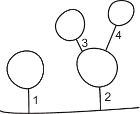
(2) if we rescale uiu_{i} on Bi​λi,k​(ci,k)B_{i\lambda_{i,k}}(c_{i,k}) to a ball of radius ii, then there is again a weak limit ωk\omega_{k} (a level 1 bubble) and finitely many bubble points so that the decomposition happens again at a higher level.

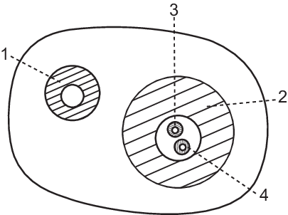
(3) Ai,k=△Bϵi,k​(ci,k)∖Bi​λi,k​(ci,k)A_{i,k}\stackrel{{\scriptstyle\triangle}}{{=}}B_{\epsilon_{i,k}}(c_{i,k})\setminus B_{i\lambda_{i},k}(c_{i,k}) is the neck region. We denote xkx_{k} by pkp_{k} and ωl​(∞)\omega_{l}(\infty) by qkq_{k}.

Refer to caption
(a) bubble tree
Refer to caption
(b) domain decomposition
Figure 1. An example

There are finitely many bubbles including the so-called ghost bubbles which are constant maps and finitely many necks. For simplicity, we label bubbles and necks by only one index. So Ai,kA_{i,k} could be a neck region at any level. Suppose there are totally LL such necks. An example of buble tree and the decomposition are illustrated in Figure 1. The shadow parts in Figure 1(b) stand for the neck regions.

We will need the following fact, which was proved during the construction of this bubble tree structure (see (1.6) in [17]): On a neck region,

(5.1) ∫Ai,ke⁡(ui)=CR<ε1/6,\int_{A_{i,k}}e(u_{i})=C_{R}<\varepsilon_{1}/6,

where ε1\varepsilon_{1} is the constant given in Lemma 5.4. To see this, recall that λi,k\lambda_{i,k} is defined to be

λi,k=largest ​λ​ such that ​∫Bϵi,k​(ci,k)∖Bλ​(ci,k)e⁡(ui)≥CR\lambda_{i,k}=\mbox{largest }\lambda\mbox{ such that }\int_{B_{\epsilon_{i,k}(c_{i,k})}\setminus B_{\lambda}(c_{i,k})}e(u_{i})\geq C_{R}

and Ai,k⊂Bϵi,k​(ci,k)∖Bλi,k​(ci,k)A_{i,k}\subset B_{\epsilon_{i,k}}(c_{i,k})\setminus B_{\lambda_{i,k}}(c_{i,k}). By choosing δ\delta small, RR large and a new subsequence if necessary, we may require

(5.2) ∫Bδ∖Bλi,k​Re⁡(ui)<ε1/3\int_{B_{\delta}\setminus B_{\lambda_{i,k}R}}e(u_{i})<\varepsilon_{1}/3

for ii large.

To prove (1.2), it suffices to show

∑k=1Llimi→∞∫Ai,ke⁡(ui)=0.\sum_{k=1}^{L}\lim_{i\to\infty}\int_{A_{i,k}}e(u_{i})=0.

5.2. An extension lemma

Let pp be a point in NN and rr be the injectivity radius of NN. Consider a map f:S1→Nf:S^{1}\to N whose image lies in Br​(p)B_{r}(p). Define f~:B2∖B1→N\tilde{f}:B_{2}\setminus B_{1}\to N as

(5.3) f~​(θ,r)=expp⁡[(2−r)​expp−1⁡f⁡(θ)].\tilde{f}(\theta,r)=\exp_{p}[(2-r)\exp_{p}^{-1}f(\theta)].

It is obvious from the definition that f~​(θ,1)=f​(θ)\tilde{f}(\theta,1)=f(\theta) and f~​(θ,2)=p\tilde{f}(\theta,2)=p. We need to compute the energy of f~\tilde{f}. The chain rule implies

|∂∂r​f~​(θ,r)|=|D​(expp)(2−r)​expp−1⁡f⁡(θ)⋅expp−1⁡f⁡(θ)|≤C​d​(f⁡(θ),p)\left|\frac{\partial}{\partial r}\tilde{f}(\theta,r)\right|=\left|D(\exp_{p})_{(2-r)\exp_{p}^{-1}f(\theta)}\cdot\exp_{p}^{-1}f(\theta)\right|\leq Cd(f(\theta),p)

and

|∂∂θ​f~​(θ,r)|=|D​(expp)(2−r)​expp−1⁡f⁡(θ)⋅(2−r)​D​(expp−1)f⁡(θ)​f′​(θ)|≤C⁡(2−r)​f′​(θ).\left|\frac{\partial}{\partial\theta}\tilde{f}(\theta,r)\right|=\left|D(\exp_{p})_{(2-r)\exp_{p}^{-1}f(\theta)}\cdot(2-r)D(\exp_{p}^{-1})_{f(\theta)}f^{\prime}(\theta)\right|\leq C(2-r)f^{\prime}(\theta).

Hence,

E⁡(f~)≤C​∫S1∫12(d​(f⁡(θ),p)2+1r2​(2−r)2​|f′​(θ)|2)​r​𝑑r​𝑑θ.E(\tilde{f})\leq C\int_{S^{1}}\int_{1}^{2}\left(d(f(\theta),p)^{2}+\frac{1}{r^{2}}(2-r)^{2}\left|f^{\prime}(\theta)\right|^{2}\right)rdrd\theta.

We summarize the computation in a lemma.

Lemma 5.1.

For any ε>0\varepsilon>0, there exists η>0\eta>0 depending only on ε\varepsilon and NN such that if f:S1→Nf:S^{1}\to N satisfies that

maxθ⁡[d⁡(f⁡(θ),p)+|f′​(θ)|]<η,\max_{\theta}[d(f(\theta),p)+\left|f^{\prime}(\theta)\right|]<\eta,

then the Dirichlet energy of f~\tilde{f} defined in (5.3) on B2∖B1B_{2}\setminus B_{1} is smaller than ε\varepsilon.

Remark 5.2.

We also need a similar result for

f~​(θ,r)=expp⁡[(r−1)​expp−1⁡f⁡(θ)].\tilde{f}(\theta,r)=\exp_{p}[(r-1)\exp_{p}^{-1}f(\theta)].

The proof is the same as that of Lemma 5.1, so we omit it.

5.3. A reference map

We will construct a map from MM to NN whose image looks like the weak limit and bubbles connected by geodesics. It keeps the record of some topological information which will later be used to construct a new minimizing sequence.

Lemma 5.3.

There exists some positive constant σ\sigma depending only on NN such that if f1,f2f_{1},f_{2} are two continuous maps from Ω\Omega into NN such that

d⁡(f1​(x),f2​(x))≤σd(f_{1}(x),f_{2}(x))\leq\sigma

for all x∈Ωx\in\Omega and f1|∂Ω=f2|∂Ωf_{1}|_{\partial\Omega}=f_{2}|_{\partial\Omega}, then there exists a homotopy deforming f1f_{1} to f2f_{2} with ∂Ω\partial\Omega fixed.

We omit the proof since it is obvious.

Lemma 5.4.

There is a positive constant ε1\varepsilon_{1} depending only on NN such that any W1,2∩C0W^{1,2}\cap C^{0} map g:S2→Ng:S^{2}\to N with E⁡(g)<ε1E(g)<\varepsilon_{1} is homotopic to a constant mapping.

Proof.

Consider the harmonic map flow g⁡(t)g(t) starting from gg. Since the energy is not enough for a bubble (if ε1\varepsilon_{1} is small) then we know the flow is smooth for all time and converges sequencially and strongly to a harmonic map g∞g_{\infty}. In [18], it is proved that the energy of such a harmonic map is no less than some constant depending only NN unless it is a constant map. By choosing ε1\varepsilon_{1} small, we may assume g∞g_{\infty} is a constant map. If tn→∞t_{n}\to\infty is a sequence of time such that g⁡(tn)g(t_{n}) converges smoothly to g∞g_{\infty}, we known from Lemma 5.3 that g⁡(tn)g(t_{n}) is homotopic to g∞g_{\infty} for nn large. Hence gg is homotopic to the constant map g∞g_{\infty}. ∎

The next lemma shows how to squeeze a little room on both ends of a long neck region without changing the energy much.

Lemma 5.5.

For ii large so that δ>>λi​R\delta>>\lambda_{i}R, there is a diffeomorphism ff from Bδ∖Bλi​RB_{\delta}\setminus B_{\lambda_{i}R} to Bδ/4∖B4​λi​RB_{\delta/4}\setminus B_{4\lambda_{i}R} such that for any map u:Bδ∖Bλi​R→Nu:B_{\delta}\setminus B_{\lambda_{i}R}\to N, we have

1−C⁡(δλi​R)≤E⁡(u∘f−1,Bδ/4∖B4​λi​R)E⁡(u,Eδ∖Eλi​R)≤1+C⁡(δλi​R),1-C(\frac{\delta}{\lambda_{i}R})\leq\frac{E(u\circ f^{-1},B_{\delta/4}\setminus B_{4\lambda_{i}R})}{E(u,E_{\delta}\setminus E_{\lambda_{i}R})}\leq 1+C(\frac{\delta}{\lambda_{i}R}),

where C⁡(δλi​R)C(\frac{\delta}{\lambda_{i}R}) is a constant which goes to zero if δλi​R\frac{\delta}{\lambda_{i}R} goes to infinity.

Proof.

By conformal invariance of the Dirichlet energy, uu can be regarded as a map from S1×[0,K]S^{1}\times[0,K] to NN, where K=δ/(λi​R)K=\delta/(\lambda_{i}R). Define f~:S1×[0,K]→S1×[4,K−4]\tilde{f}:S^{1}\times[0,K]\to S^{1}\times[4,K-4] by

f~​(θ,ρ)=(θ,4+ρ​K−8K).\tilde{f}(\theta,\rho)=(\theta,4+\rho\frac{K-8}{K}).

It is straightforward to check

1−C⁡(K)≤E⁡(u∘f~−1,S1×[4,K−4])E⁡(u,S1×[0,K])≤1+C⁡(K),1-C(K)\leq\frac{E(u\circ\tilde{f}^{-1},S^{1}\times[4,K-4])}{E(u,S^{1}\times[0,K])}\leq 1+C(K),

for some C⁡(K)C(K) such that C⁡(K)C(K) goes to zero if KK goes to infinity. Set s:S1×[0,K]→Bδ∖Bλi​Rs:S^{1}\times[0,K]\to B_{\delta}\setminus B_{\lambda_{i}R} to be

s⁡(θ,ρ)=(θ,λi​R​eρ).s(\theta,\rho)=(\theta,\lambda_{i}Re^{\rho}).

Then f:Bδ∖Bλi​R→Bδ/4∖B4​λi​Rf:B_{\delta}\setminus B_{\lambda_{i}R}\to B_{\delta/4}\setminus B_{4\lambda_{i}R} defined by

f=s∘f~∘s−1f=s\circ\tilde{f}\circ s^{-1}

is the diffeomorphism we need. ∎

A remark about the notation is needed for the rest of the proof. For simplicity, we omit the subscript for necks as if there was only one neck. In fact, one should repeat the construction or proof for each neck region. By the nature of the following proof, this should cause no further difficulty. We write Bδ∖Bλi​RB_{\delta}\setminus B_{\lambda_{i}R} for a neck region, omitting the center. We assume the neck connects the weak limit and a level 1 bubble. For a general neck, one should replace uu with some bubble map ωj\omega_{j}.

We need δ\delta, RR and ii to satisfy the following conditions.

(A1) Let ε=min⁡{ε1,ξ/L}/8\varepsilon=\min\{\varepsilon_{1},\xi/L\}/8, where ξ\xi is a positive number introduced in the next subsection and LL is the total number of necks. Lemma 5.1 gives an η\eta. Choose δ\delta and RR so that for each neck region Bδ∖Bλi​RB_{\delta}\setminus B_{\lambda_{i}R}, uu restricted to ∂Bδ\partial B_{\delta} satisfies

(5.4) maxθ⁡|d⁡(u,p)|+|dd​θ​u|≤min⁡{η/2,σ/2}\max_{\theta}\left|d(u,p)\right|+\left|\frac{d}{d\theta}u\right|\leq\min\{\eta/2,\sigma/2\}

where pp is the value of uu at the bubble point and ω\omega restricted to ∂BR⊂ℝ2\partial B_{R}\subset\mathbb{R}^{2} satisfies

(5.5) maxθ⁡|d⁡(ω,q)|+|dd​θ​ω|≤min⁡{η/2,σ/2},\max_{\theta}\left|d(\omega,q)\right|+\left|\frac{d}{d\theta}\omega\right|\leq\min\{\eta/2,\sigma/2\},

where qq is limx→∞ω⁡(x)\lim_{x\to\infty}\omega(x). Fix δ\delta and RR, choose some ii so large that

(A2) (5.4) and (5.5) remains true if we replace uu by uiu_{i}, ω\omega by ui(λi⋅)u_{i}(\lambda_{i}\cdot), η/2\eta/2 by η\eta and σ/2\sigma/2 by σ\sigma;

(A3) |ui−u|≤σ/3\left|u_{i}-u\right|\leq\sigma/3 for x∈M∖Bδx\in M\setminus B_{\delta} and |ui​(λi​x)−ω⁡(x)|≤σ/3\left|u_{i}(\lambda_{i}x)-\omega(x)\right|\leq\sigma/3 for all x∈BRx\in B_{R} where σ\sigma is the constant in Lemma 5.3;

(A4) Let C⁡(⋅)C(\cdot) be the function given in Lemma 5.5. Let ii be so large that 1+C⁡(δλi​R)<21+C(\frac{\delta}{\lambda_{i}R})<2.

Now we define a new map w:M→Nw:M\to N so that

(1) w=uiw=u_{i} on M∖BδM\setminus B_{\delta} and Bλi​RB_{\lambda_{i}R};

(2) w=ui∘f−1w=u_{i}\circ f^{-1} on Bδ/4∖B4​λi​RB_{\delta/4}\setminus B_{4\lambda_{i}R}, where ff is the diffeomorphism constructed in Lemma 5.5;

(3) w⁡(θ,r)=expp⁡[r−δ/2δ/2​expp−1​ui​(θ,δ)]w(\theta,r)=\exp_{p}[\frac{r-\delta/2}{\delta/2}\exp_{p}^{-1}u_{i}(\theta,\delta)] for (θ,r)∈Bδ∖Bδ/2(\theta,r)\in B_{\delta}\setminus B_{\delta/2};

(4) w⁡(θ,r)=w⁡(θ,δ24​r)w(\theta,r)=w(\theta,\frac{\delta^{2}}{4r}) for (θ,r)∈Bδ/2∖Bδ/4(\theta,r)\in B_{\delta/2}\setminus B_{\delta/4};

(5) w⁡(θ,r)=expq⁡[2​λi​R−rλi​R​expq−1​ui​(θ,λi​R)]w(\theta,r)=\exp_{q}[\frac{2\lambda_{i}R-r}{\lambda_{i}R}\exp_{q}^{-1}u_{i}(\theta,\lambda_{i}R)] for (θ,r)∈B2​λi​R∖Bλi​R(\theta,r)\in B_{2\lambda_{i}R}\setminus B_{\lambda_{i}R};

(6) w⁡(θ,r)=w⁡(θ,(2​λi​R)2r)w(\theta,r)=w(\theta,\frac{(2\lambda_{i}R)^{2}}{r}) for (θ,r)∈B4​λi​R∖B2​λi​R(\theta,r)\in B_{4\lambda_{i}R}\setminus B_{2\lambda_{i}R}.

It is easy to see that ww is homotopic to uiu_{i}. Now let us consider the map ww restricted to Bδ/2∖B2​λi​RB_{\delta/2}\setminus B_{2\lambda_{i}R}. It follows from the construction that ww maps ∂Bδ/2\partial B_{\delta/2} to pp and ∂B2​λi​R\partial B_{2\lambda_{i}R} to qq. Hence, topologically it induces a map from S2S^{2} to NN if we identify ∂B2​λi​R\partial B_{2\lambda_{i}R} with the north pole PNP_{N} and ∂Bδ/2\partial B_{\delta/2} with the south pole PSP_{S}. This is in fact a homotopically trivial map. To see this, consider a map w1:ℝ2→Nw_{1}:\mathbb{R}^{2}\to N which agrees with ww on Bδ/2∖2​λi​RB_{\delta/2}\setminus 2\lambda_{i}R and maps B2​λi​RB_{2\lambda_{i}R} to qq and ℝ2∖Bδ/2\mathbb{R}^{2}\setminus B_{\delta/2} to pp. By the conformal invariance of EE, we regard w1w_{1} as a map from S2S^{2} to NN. By (A1), (A2) (A4) and (5.2) , the energy of this map is smaller than ε1\varepsilon_{1} in Lemma 5.4, hence it is homotopic to a constant map. Let F:S2×[0,1]→NF:S^{2}\times[0,1]\to N be the homotopy such that F⁡(⋅,0)=w1​(⋅)F(\cdot,0)=w_{1}(\cdot), F⁡(⋅,1)≡pF(\cdot,1)\equiv p and F⁡(PS,t)=pF(P_{S},t)=p for any t∈[0,1]t\in[0,1]. The curve F⁡(PN,⋅)F(P_{N},\cdot) connects qq and pp. Let γ:[0,1]→N\gamma:[0,1]\to N be the shortest geodesic homotopic to this curve connecting qq and pp.

Refer to caption
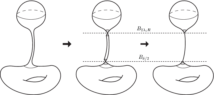
Figure 2. reference map

We can now define the reference map w~\tilde{w}. Let w~=w\tilde{w}=w except that on Bδ/2∖B2​λi​RB_{\delta/2}\setminus B_{2\lambda_{i}R}

w~​(θ,r)=γ⁡(log⁡r−log⁡(2​λi​R)log⁡(δ/2)−log⁡(2​λi​R)).\tilde{w}(\theta,r)=\gamma(\frac{\log r-\log(2\lambda_{i}R)}{\log(\delta/2)-\log(2\lambda_{i}R)}).

The above construction is illustrated by Figure 2. We claim that ww and w~\tilde{w} are homotopic. Since ww and w~\tilde{w} are the same except on B2​δ∖B2​λi​RB_{2\delta}\setminus B_{2\lambda_{i}R}, we construct the homotopy explicitly. For (θ,r)∈Bδ/2∖B2​λi​R(\theta,r)\in B_{\delta/2}\setminus B_{2\lambda_{i}R},

G⁡((θ,r),s)={F⁡(PN,r−2​λi​Rδ/2−2​λi​R),2​λi​R≤r≤r⁡(s)F⁡((θ,(δ/2−2​λi​R)​r−r⁡(s)δ/2−r⁡(s)+2​λi​R),s),r⁡(s)≤r≤δ/2,G((\theta,r),s)=\left\{\begin{array}[]{ll}F(P_{N},\frac{r-2\lambda_{i}R}{\delta/2-2\lambda_{i}R}),&2\lambda_{i}R\leq r\leq r(s)\\ F((\theta,(\delta/2-2\lambda_{i}R)\frac{r-r(s)}{\delta/2-r(s)}+2\lambda_{i}R),s),&r(s)\leq r\leq\delta/2,\end{array}\right.

where r⁡(s)=2​λi​R+s⁡(δ/2−2​λi​R)r(s)=2\lambda_{i}R+s(\delta/2-2\lambda_{i}R). From here, it is obvious that one can further deform F⁡(PN,t)F(P_{N},t) to γ\gamma.

If there are more than one neck region, we repeat the above construction for each neck.

5.4. Proof of the energy identity

Let us assume that the energy identity (1.2) is not true. Then there exists ξ>0\xi>0 and a subsequence (still denoted by uiu_{i}) such that

limi→∞∑k=1L∫Ai,ke⁡(ui)≥ξ.\lim_{i\to\infty}\sum_{k=1}^{L}\int_{A_{i,k}}e(u_{i})\geq\xi.

Let w~\tilde{w} be the reference map constructed above. We will show a contradiction by construct a new sequence u~i\tilde{u}_{i} in the same homotopy class such that

limi→∞E⁡(u~i)<limi→∞E⁡(ui).\lim_{i\to\infty}E(\tilde{u}_{i})<\lim_{i\to\infty}E(u_{i}).

Define u~i\tilde{u}_{i} as follows

(1) u~i=ui\tilde{u}_{i}=u_{i} outside the neck region (Bδ∖Bλi​RB_{\delta}\setminus B_{\lambda_{i}R});

(2) u~i​(θ,r)=expp⁡[r−δ/2δ/2​expp−1​ui​(θ,δ)]\tilde{u}_{i}(\theta,r)=\exp_{p}[\frac{r-\delta/2}{\delta/2}\exp_{p}^{-1}u_{i}(\theta,\delta)] for (θ,r)∈Bδ∖Bδ/2(\theta,r)\in B_{\delta}\setminus B_{\delta/2};

(3) u~i​(θ,r)=expq⁡[2​λi​R−rλi​R​expp−1​ui​(θ,λi​R)]\tilde{u}_{i}(\theta,r)=\exp_{q}[\frac{2\lambda_{i}R-r}{\lambda_{i}R}\exp_{p}^{-1}u_{i}(\theta,\lambda_{i}R)] for (θ,r)∈B2​λi​R∖Bλi​R(\theta,r)\in B_{2\lambda_{i}R}\setminus B_{\lambda_{i}R};

(4) u~i​(θ,r)=γ⁡(log⁡r−log⁡(2​λi​R)log⁡(δ/2)−log⁡(2​λi​R))\tilde{u}_{i}(\theta,r)=\gamma(\frac{\log r-\log(2\lambda_{i}R)}{\log(\delta/2)-\log(2\lambda_{i}R)}).

It remains to show first, the energy of ui~\tilde{u_{i}} in the neck region is smaller than ξ/2\xi/2 for ii large and second, u~i\tilde{u}_{i} is homotopic to w~\tilde{w}. For the first point, (A1) and Lemma 5.1 implies that the energy in Bδ∖Bδ/2B_{\delta}\setminus B_{\delta/2} and B2​λi​R∖Bλi​RB_{2\lambda_{i}R}\setminus B_{\lambda_{i}R} for all necks is no more than ξ/4\xi/4. Moreover, as ii gets larger, then the energy on the geodesic part can be made as small as we want since the length of γ\gamma is fixed (See Section 5.3).

For the second point, if there is only one neck, then MM is decomposed into three parts; M∖Bδ/2M\setminus B_{\delta/2}, Bδ/2∖B2​λi​RB_{\delta/2}\setminus B_{2\lambda_{i}R} and B2​λi​RB_{2\lambda_{i}R}. For the reference map w~\tilde{w}, the decomposition is fixed because we chose and fixed a large ii in the construction. For ui~\tilde{u_{i}}, the center of BδB_{\delta} and Bλi​RB_{\lambda_{i}R} changes with ii and so does the radius of B2​λi​RB_{2\lambda_{i}R}. However, when restricted to the separating circles ∂Bδ/2\partial B_{\delta/2} and ∂B2​λi​R\partial B_{2\lambda_{i}R}, w~\tilde{w} and u~i\tilde{u}_{i} are constant maps to the same points. This allows us to prove the homotopy between w~\tilde{w} and u~i\tilde{u}_{i} on each of the three parts separately.

On M∖Bδ/2M\setminus B_{\delta/2}, (A1) and (A3) show that d⁡(w~,u~i)<σd(\tilde{w},\tilde{u}_{i})<\sigma, which implies that there is a homotopy between them leaving ∂Bδ/2\partial B_{\delta/2} fixed. The bubble part B2​λi​RB_{2\lambda_{i}R} of w~\tilde{w} and u~i\tilde{u}_{i} are homotopic for the same reason. On Bδ/2∖B2​λi​RB_{\delta/2}\setminus B_{2\lambda_{i}R} part, they are different parametrization of the same curve. This concludes our proof for (1.2) in the case of only one neck.

For the general case of multiple necks, the decomposition is more complicated but the same argument applies. To illustrate the idea, consider a bubble tree as shown in Figure 1(a). The necks are labelled from 11 to 44. The corresponding decomposition of MM is illustrated in Figure 1(b). The shadow parts are neck regions. There are eight circles separating the neck regions and the bubble regions. Both w~\tilde{w} and u~i\tilde{u}_{i} map these circles to pip_{i}’s and qiq_{i}’s. The homotopy for bubble regions (including M∖(Bδ/2​(x1)∪Bδ/2​(x2))M\setminus(B_{\delta/2}(x_{1})\cup B_{\delta/2}(x_{2})) follows from Lemma 5.3 and the homotopy for neck regions is obvious because they are different parametrization of the same geodesics.

6. Appendix

In this appendix, we prove the local existence and uniqueness of the α−\alpha-flow equation

(6.1) ∂tu=△M​u+(α−1)​∇|∇u|2⋅∇u1+|∇u|2+A⁡(u)​(∇u,∇u)\partial_{t}u=\triangle_{M}u+(\alpha-1)\frac{\nabla\left|\nabla u\right|^{2}\cdot\nabla u}{1+\left|\nabla u\right|^{2}}+A(u)(\nabla u,\nabla u)

for any smooth initial value u0:M→N⊂ℝku_{0}:M\to N\subset\mathbb{R}^{k}.

As in the case of harmonic maps, there is an intrinsic way of writing the right hand side of (6.1). If we regard (1+|∇u|2)α−1∇u(1+\left|\nabla u\right|^{2})^{\alpha-1}\nabla u as a section of the pull back bundle u∗​T​Nu^{*}TN and denote the induced connection of u∗​T​Nu^{*}TN by D~\tilde{D}, the righthand side can be written as

τα​(u):=1(1+|∇u|2)α−1​∑iD~ei​((1+|∇u|2)α−1​∇eiu),\tau_{\alpha}(u):=\frac{1}{(1+\left|\nabla u\right|^{2})^{\alpha-1}}\sum_{i}\tilde{D}_{e_{i}}\left((1+\left|\nabla u\right|^{2})^{\alpha-1}\nabla_{e_{i}}u\right),

where {ei}\{e_{i}\} is an orthonormal basis of T​MTM in some open set. In the following, we will call τα\tau_{\alpha} the α−\alpha-tension field of uu. It is obvious that smooth solution to (6.1) is equivalent to that of the following

∂u∂t=τα​(u),\frac{\partial u}{\partial t}=\tau_{\alpha}(u),

where we regard u⁡(⋅,t)u(\cdot,t) as maps into NN. This allows us to consider a totally geodesic isometric embedding of NN into ℝk\mathbb{R}^{k} with some non-flat metric as in [9]. Precisely, there is a metric hh on ℝk\mathbb{R}^{k} and an embedding NN into ℝk\mathbb{R}^{k} such that the isometric embedding is totally geodesic and there exists an isometric involution ii which acts on a tubular neighborhood 𝒯\mathcal{T} of NN, leaving points of NN fixed. By composing with this embedding, we regard uu as a map from MM into (ℝk,h)(\mathbb{R}^{k},h) and denote by ταN\tau_{\alpha}^{N} and ταℝk\tau_{\alpha}^{\mathbb{R}^{k}} the α−\alpha-tension fields of uu as a map into NN and into ℝk\mathbb{R}^{k} respectively. Since NN is a totally geodesic submanifold, we have ταN​(u)=ταℝk​(u)\tau_{\alpha}^{N}(u)=\tau_{\alpha}^{\mathbb{R}^{k}}(u) (see page 108 in [9]). Therefore, it suffices to study

(6.2) ∂uβ∂t=△Muβ+(α−1)∇|∇u|2⋅∇uβ1+|∇u|2+Γ(u)#∇u#∇u,\frac{\partial u^{\beta}}{\partial t}=\triangle_{M}u^{\beta}+(\alpha-1)\frac{\nabla\left|\nabla u\right|^{2}\cdot\nabla u^{\beta}}{1+\left|\nabla u\right|^{2}}+\Gamma(u)\#\nabla u\#\nabla u,

where uβu^{\beta} is the components of uu, △M\triangle_{M} is the usual Laplacian on MM and Γ\Gamma is the Christoffel symbol of the Levi-Civita connection of (ℝk,h)(\mathbb{R}^{k},h). Since |∇u|2=hβ​γ(u)∇uβ⋅∇uγ\left|\nabla u\right|^{2}=h_{\beta\gamma}(u)\nabla{u^{\beta}}\cdot\nabla{u^{\gamma}}, when we expand ∇|∇u|2\nabla\left|\nabla u\right|^{2}, there is an extra term involving the gradient of h⁡(u)h(u) which can be absorbed into the last term. The equation can be rewritten as

(6.3) ∂uβ∂t=△Muβ+2(α−1)∇i​j2uγ​∇iuγ​∇juβ1+|∇u|2+Γ~(u)#∇u#∇u.\frac{\partial u^{\beta}}{\partial t}=\triangle_{M}u^{\beta}+2(\alpha-1)\frac{\nabla^{2}_{ij}u^{\gamma}\nabla_{i}u^{\gamma}\nabla_{j}u^{\beta}}{1+\left|\nabla u\right|^{2}}+\tilde{\Gamma}(u)\#\nabla u\#\nabla u.

Next, we start a routine iteration procedure to show the local existence of (6.3). Consider the following linear parabolic system

(6.4) ∂u∂t=△u+(α−1)(∇2u,∇v)∇v1+|∇v|2+Γ~(v)#∇v#∇v.\frac{\partial u}{\partial t}=\triangle u+(\alpha-1)\frac{(\nabla^{2}u,\nabla v)\nabla v}{1+\left|\nabla v\right|^{2}}+\tilde{\Gamma}(v)\#\nabla v\#\nabla v.

Let w=u−u0w=u-u_{0}, then ww satisfies

(6.5) ∂w∂t\displaystyle\frac{\partial w}{\partial t} =\displaystyle= △w+(α−1)(∇2w,∇v)∇v1+|∇v|2+Γ~(v)#∇v#∇v\displaystyle\triangle w+(\alpha-1)\frac{(\nabla^{2}w,\nabla v)\nabla v}{1+\left|\nabla v\right|^{2}}+\tilde{\Gamma}(v)\#\nabla v\#\nabla v
+△​u0+(α−1)​(∇2u0,∇v)∇v1+|∇v|2.\displaystyle+\triangle u_{0}+(\alpha-1)\frac{(\nabla^{2}u_{0},\nabla v)\nabla v}{1+\left|\nabla v\right|^{2}}.

For some μ∈(1,2)\mu\in(1,2), set

V={v∈Cμ,μ/2(M×[0,T])|‖v‖Cμ,μ/2​(M×[0,T])≤1,v(0)≡0}.V=\left\{v\in C^{\mu,\mu/2}(M\times[0,T])|\quad\left\|v\right\|_{C^{\mu,\mu/2}(M\times[0,T])}\leq 1,v(0)\equiv 0\right\}.

For each v∈Vv\in V, the Schauder estimate of linear parabolic systems (see [8] and [19]) implies

(6.6) ‖w‖Cμ+1,μ+12​(M×[0,T])≤C⁡(‖w‖C0​(M×[0,T])+‖u0‖Cμ+1​(M)+1).\left\|w\right\|_{C^{\mu+1,\frac{\mu+1}{2}}(M\times[0,T])}\leq C(\left\|w\right\|_{C^{0}(M\times[0,T])}+\left\|u_{0}\right\|_{C^{\mu+1}(M)}+1).

Since w⁡(⋅,0)≡0w(\cdot,0)\equiv 0, we have

‖w‖C0​(M×[0,T])≤T​C​(‖w‖C0​(M×[0,T])+‖u0‖Cμ+1​(M)+1).\left\|w\right\|_{C^{0}(M\times[0,T])}\leq TC(\left\|w\right\|_{C^{0}(M\times[0,T])}+\left\|u_{0}\right\|_{C^{\mu+1}(M)}+1).

Choose TT small so that

‖w‖C0​(M×[0,T])≤T​C​(‖u0‖Cμ+1​(M)+1).\left\|w\right\|_{C^{0}(M\times[0,T])}\leq TC(\left\|u_{0}\right\|_{C^{\mu+1}(M)}+1).

By the interpolation of the Hölder space, for σ>0\sigma>0 such that μ=(1−σ)​(μ+1)\mu=(1-\sigma)(\mu+1), we have

‖w‖Cμ,μ/2​(M×[0,T])≤‖w‖C0​(M×[0,T])σ​‖w‖Cμ+1,μ+12​(M×[0,T])1−σ.\left\|w\right\|_{C^{\mu,\mu/2}(M\times[0,T])}\leq\left\|w\right\|_{C^{0}(M\times[0,T])}^{\sigma}\left\|w\right\|_{C^{\mu+1,\frac{\mu+1}{2}}(M\times[0,T])}^{1-\sigma}.

This implies that we can choose TT sufficiently small so that w∈Vw\in V.

Now start from any v0∈Vv_{0}\in V. Let vk+1v_{k+1} be the solution of (6.4) with v=vkv=v_{k} and zero initial value. We then have a uniform bound

‖vk‖Cμ+1,μ+12​(M×[0,T])≤C.\left\|v_{k}\right\|_{C^{\mu+1,\frac{\mu+1}{2}}(M\times[0,T])}\leq C.

Using Schauder estimate again, we obtain uniform Cμ+3,μ+32C^{\mu+3,\frac{\mu+3}{2}} estimate for vkv_{k}. By taking a subsequence, we know vkv_{k} converges to some ww in Cμ+1,μ+12​(M×[0,T])C^{\mu+1,\frac{\mu+1}{2}}(M\times[0,T]). Then w+u0w+u_{0} is a solution to the α−\alpha-flow with initial value u0u_{0}.

If there are two smooth solutions uu and ww to the equation (6.3) defined on [0,T][0,T], we can subtract the two equations, multiply both sides by u−wu-w and integrate over MM to get

12​dd​t​∫M|w−u|2​𝑑v\displaystyle\frac{1}{2}\frac{d}{dt}\int_{M}\left|w-u\right|^{2}dv ≤\displaystyle\leq −∫M|∇(u−w)|2dv\displaystyle-\int_{M}\left|\nabla(u-w)\right|^{2}dv
+2(α−1)∫M(∇i​j2(uβ−wβ))uiβ​ujγ1+|∇u|2(uγ−wγ)dv\displaystyle+2(\alpha-1)\int_{M}(\nabla^{2}_{ij}(u^{\beta}-w^{\beta}))\frac{u^{\beta}_{i}u^{\gamma}_{j}}{1+\left|\nabla u\right|^{2}}(u^{\gamma}-w^{\gamma})dv
+C∫M|u−w|2dv+C∫M|∇u−∇w||u−w|dv.\displaystyle+C\int_{M}\left|u-w\right|^{2}dv+C\int_{M}\left|\nabla u-\nabla w\right|\left|u-w\right|dv.

For the second term in the right hand side, integrating by parts and noticing that uiβ​ujγ1+|∇u|2​∇i(uβ−wβ)​∇j(uγ−wγ)≥0\frac{u^{\beta}_{i}u^{\gamma}_{j}}{1+\left|\nabla u\right|^{2}}\nabla_{i}(u^{\beta}-w^{\beta})\nabla_{j}(u^{\gamma}-w^{\gamma})\geq 0 yields

dd​t​∫M|u−w|2​𝑑v≤C​∫M|u−w|2​𝑑v,\frac{d}{dt}\int_{M}\left|u-w\right|^{2}dv\leq C\int_{M}\left|u-w\right|^{2}dv,

which implies u≡wu\equiv w on M×[0,T]M\times[0,T] if u=wu=w for t=0t=0. It follows immediately from the uniqueness and the involution isometry i:𝒯→𝒯i:\mathcal{T}\to\mathcal{T} that if u0u_{0} is a map from MM to NN, the image of the local solution u⁡(x,t)u(x,t) obtained above lies in NN.

Acknowledgement 1.

The research of the first author was supported by the Australian Research Council grant DP0985624. The second author was supported by a postdoctoral fellowship at the University of Queensland through the grant DP0985624.

References

  • [1] M. Bertsch, R. Dal Passo, R. Van der Hout: Nonuniqueness for the heat flow of harmonic maps on the disk, Arch. Ration. Mech. Anal., 161 (2002), no.2, 93-112.
  • [2] K.C. Chang, W.Y. Ding, R. Ye: Finite-time blow-up of the heat flow of harmonic maps from surfaces, J. Differential Geom., 36 (1992), no.2, 507-515.
  • [3] J.Y. Chen, G. Tian: Compactification of moduli space of harmonic mappings, Comment. Math. Helv., 74 (1999), 201-237.
  • [4] Y.M. Chen, M. Struwe: Existence and partial regularity for heat flow for hamonic maps, Math. Z., 201 (1989), 83-103.
  • [5] W.Y. Ding, G. Tian: Energy identity for a class of approximate harmonic maps from surfaces, Comm. Anal. Geom., 3 (1996), 543-554.
  • [6] F. Duzaar, E. Kuwert: Minimization of conformal invariant energies in homotopy classes, Calc. Var. Partial Differential Equations, 6 (1998), no.4, 285-313.
  • [7] J. Eells, J.H. Sampson: harmonic mappings of Riemannian manifolds, Amer. J. Math., 86 (1964) 109-160.
  • [8] S.D. Eidel’man: Parabolic systems, Translated from the Russian by Scripta Technica, London North-Holland Publishing Co., Amsterdam-London; Wolters-Noordhoff Publishing, Groningen 1969.
  • [9] R.S. Hamilton: Harmonic maps of manifolds with boundary, Lecture Notes in Mathematics, Vol. 471, Springer-Verlag, Berlin-New York, 1975.
  • [10] T. Lamm: Energy identity for approximations of harmonic maps from surfaces, Trans. Amer. Math. Soc., 362 (2010), 4077-4097.
  • [11] L. Lemaire: Applications harmoniques des surfaces Riemanniennes, J. Differential Geom., 13 (1978), 51-78.
  • [12] J.Y. Li, G. Tian: The blow-up locus of heat flows for harmonic maps, Acta Math. Sin. (Engl. Ser.), 16 (2000), no.1, 29-62.
  • [13] Y.X. Li, Y.D. Wang: A weak energy identity and the length of necks for a sequence of Sacks-Uhlenbeck α\alpha-harmonic maps, Adv. Math. (2010), doi:10.1016/j.aim.2010.03.020.
  • [14] Y.X. Li, Y.D. Wang: Bubbling location for sequences of approximate f−f-harmonic maps from surfaces; Internat. J. Math., 21 (2010), no.4, 475-495.
  • [15] F.H. Lin, C.Y. Wang: Harmonic and quasi-harmonic spheres, Comm. Anal. Geom., 7 (1999), no.2, 397-429.
  • [16] F.H. Lin, C.Y. Wang: The analysis of harmonic maps and their heat flows, World Scientific Publishing Co. Pte. Ltd. (2008).
  • [17] T. Parker: Bubble tree convergence for harmonic maps, J. Differential Geom., 44 (1996), 595-633.
  • [18] J. Sacks, K. Uhlenbeck: The existence of minimal immersions of 2−2-spheres, Ann. of Math. (2), 113 (1981), no.1, 1-24.
  • [19] W. Schlag: Schauder and LpL^{p} estimates for parabolic systems via companato spaces, Comm. Partial Differential Equations, 21 (1996), no. 7-8, 1141-1175.
  • [20] R. Schoen: Analytic aspects of the harmonic map problem, Seminar on nonlinear partial differential equations (Berkeley, Calif., 1983), 321-358, Math. Sci. Res. Inst. Publ., 2, Springer, New York, 1984.
  • [21] R. Schoen, S.T. Yau: Existence of incompressible minimal surfaces and the topology of three dimensional manifolds with non-negative scalar curvature, Ann. of Math., 110 (1979), 127-142.
  • [22] M. Struwe: On the evolution of harmonic maps of Riemannian surfaces, Comm. Math. Helv., 60 (1985), 558-581.
  • [23] M. Struwe: On the evolution of harmonic maps in higher dimensions, J. Differential Geom., 28 (1988), 485-502.
  • [24] P. Topping: Reverse bubbling and nonuniqueness in the harmonic map flow, Int. Math. Res. Not., (2002) no.10, 505-520.