The method of Gaussian weighted trajectories.
V.
On the 1GB procedure for polyatomic processes
Abstract
In recent years, many chemical reactions have been studied by means of the quasi-classical trajectory (QCT) method within the Gaussian binning (GB) procedure. The latter consists in "quantizing" the final vibrational actions in Bohr spirit by putting strong emphasis on the trajectories reaching the products with vibrational actions close to integer values. A major drawback of this procedure is that if is the number of product vibrational modes, the amount of trajectories necessary to converge the calculations is larger than with the standard QCT method. Applying it to polyatomic processes is thus problematic. In a recent paper, however, Czakó and Bowman propose to quantize the total vibrational energy instead of the vibrational actions [G. Czakó and J. M. Bowman, J. Chem. Phys., 131, 244302 (2009)], a procedure called 1GB here. The calculations are then only 10 times more time-consuming than with the standard QCT method, allowing thereby for considerable numerical saving. In this paper, we propose some theoretical arguments supporting the 1GB procedure and check its validity on model test cases as well as the prototype four-atom reaction OH+D2 HOD+D.
I Introduction
Improving our ability to accurately describe gas-phase chemical reactions and inelastic collisions is a stimulating theoretical issue at the interface of physics and chemistry [1] and a necessary step towards a deep understanding of the evolution of planetary atmospheres and interstellar clouds.
Assuming that for a given process, the electronic problem has been solved [2], i.e., the potential energy of interaction between nuclei is known, nuclear motions can be studied either quantum [3, 4, 5, 6, 7, 8, 9, 10] or classical mechanically [11, 12]. For the present time, however, quantum scattering approaches can hardly be applied to more than three-atom processes, despite current computer performances and a great deal of methodological effort made to go beyond the triatomic problem [13, 14, 15, 16, 17].
On the other hand, the classical approach, well known as the quasi-classical trajectory method (QCTM) [11, 12], is much less time consuming and can therefore be applied to almost any process, independently on the number of atoms involved. We focus our attention on this method in the present paper.
A major goal of QCTM is to predict the distributions of the translational energy between bimolecular collision or photodissociation products as well as the distribution of their quantum states [1]. These distributions, measured in molecular beam experiments, are among the most refined data on chemical reactivity and molecular reaction dynamics. In this work, we concentrate on the possible descriptions of these two quantities within QCTM.
In its standard implementation, QCTM deals with the standard binning (SB) procedure (or histogram method) for assigning trajectories to the various quantum states available. In order to introduce this procedure, we consider the three-atom exchange reaction of the type A + BC AB + C. If at the end of a given reactive trajectory, the vibrational action of AB is in units of (see appendix A for the mathematical definition of ) and its rotational angular momentum is in units of , the trajectory is assumed to only contribute to the AB quantum state where and are the nearest integers of and respectively (in the following, the nearest integer of any variable will also be denoted by the variable with a bar on top of it).
About ten years ago, however, it was suggested
that such a procedure might lead to wrong predictions when the energy available to the
products is too low for the quantum and classical densities of product states to be equal, or equivalently,
when the available quantum states are widely spaced as compared to the energy disposal [18].
A Gaussian Binning (GB) procedure was then proposed [18] which amounts to assigning to each trajectory a Gaussian
statistical weight such that the closer the final actions to their nearest integers, the larger the weight
(by action, we mean here both vibrational actions and rotational angular momenta in the previously defined units).
For the previous triatomic process, the Gaussian weight of the trajectory ending with is
| (1) |
with
| (2) |
being usually kept at 0.05 [19, 20, 21]. Like in the SB procedure, trajectories do only contribute to the quantum state defined by the center of the bin or unit square in which stands. The GB procedure is therefore a practical way of taking into account Bohr quantization in the analysis of the final results. The GB procedure turns out to be a reminiscence of the use of narrow boxes proposed by Ron et al in the early 80’s [22], a method apparently ignored or forgotten by QCTM users.
Initially proposed on the basis of intuitive arguments, the GB procedure was later shown to be a practical implementation of classical S matrix theory (CSMT) in the random phase approximation [23, 24], CSMT being the first and simplest (or least complex) semi-classical approach of molecular collisions pioneered by Miller and Marcus in the early seventies [25, 26, 27, 28, 29, 30, 31].
The Gaussian weight is characterized by a full width at half maximum of 10 percent. This means that the values of and respectively in the ranges and mostly contribute to the GB population of the level , as compared with the values in the unit ranges and which contribute to the SB population. Therefore, the area in the plane contributing to the GB population is 100 times smaller than the one contributing to the SB population and it is necessary to run 100 times more trajectories within the GB procedure than within the SB one for the same level of convergence of the final results.
In many experiments, however, the number of available rotational states of AB is significantly larger than the number of its vibrational states (more than 10 against less than 3) and one arrives at the same result when weighting the trajectories by Eq. (1) or by alone. Within this partial GB procedure, corresponding to Eqs. (13) and (14) of reference 24, it is thus sufficient to run 10 times more trajectories than within the HB one [19, 20, 21, 24, 32, 33, 34, 35].
However, considering polyatomic reactions where the number of vibrational modes is easily ten or more, strongly clouds the situation. The reason is that "quantizing" modes amounts to weight the trajectories by a product of Gaussians. Therefore, one is led to run times more trajectories within the GB procedure than within the SB one. For the reaction F+CH FH+CH3 and its isotopic variants, much studied experimentally in the recent years [36], the previous number is 10 millions ! Since one needs at least a few hundreds of thousands of trajectories within the HB procedure, one should run a few trillions of trajectories within the GB procedure, which is just not feasible.
In order to circumvent this difficulty, Czakó and Bowman recently proposed to weight the trajectories by
(see Eq. (2)) with
| (3) |
being the vibrational action for the mode and the corresponding frequency [37]. In other words, they proposed to quantize, with one Gaussian only, the total vibrational energy (in the harmonic approximation) instead of the vibrational actions. Consequently, this 1GB procedure allows for a huge amount of computational savings for large systems.
The goal of the present paper is to propose theoretical arguments supporting this procedure and check its validity on model as well as actual processes.
The paper is organized as follows. In section II, the 1GB procedure is shown to be equivalent to the usual GB procedure for statistical collinear processes. We then discuss the conditions for its validity in the general case. The predictions to which it leads are compared in section III with the usual SB and GB predictions for a model test case involving three vibrational modes. In section IV, the approach is applied to the prototype four-body chemical reaction OH+D HOD+D which is among the simplest polyatomic bimolecular reactions [38, 39, 40, 41, 42, 43, 44]. We finally conclude in section V.
II Theoretical analysis of the 1GB procedure
In a first step, we focus our attention on collinear processes in the course of which nuclei keep on a line fixed in the laboratory frame. The realistic three-dimensional case where rotation motions are active is considered in a second step.
II.1 Collisional system involving two vibrational modes
Consider the collinear inelastic collision between atom A and the triatomic molecule BCD at the classically available energy
with respect to the free fragments. Assuming that the harmonic approximation is valid for the intra-molecular motion of BCD,
its vibrational energy at the end of the collision reads (see appendix A)
| (4) |
where and are the energy spacings between neighboring states for the two vibrational streching normal modes of BCD and and are their related actions (since B, C and D are aligned, the usual bending vibration is ignored).
The relative translational energy between A and BCD satisfies the identity
| (5) |
We call the classical distribution of the actions and , supposed to be normalized to unity.
Additional paragraph 1:
We shall consider the formal expressions of both the translational energy distribution of the final products and the one of their
quantum states. However, we shall only represent the former distribution in the figures. We might have done the contrary, but the
translational energy distribution is by far the most widely measured in molecular beam experiments. We thus believe that discussing
the different ways this distribution can be represented in QCT studies is an important issue.
In addition to that, the translational and internal energies being mathematically related (see Eq. (5)), the two distributions
can, in principle, be deduced from each other. In this section and the next one, for instance, it will turn out that
the product state distribution is readily obtained from visual inspection of the translational energy distribution.
End of the additional paragraph 1.
II.2 Purely classical translational energy distribution
The translational energy distribution obtained from a strict application of classical mechanics reads
| (6) |
(see appendix B for its derivation). Since this density has no quantum attribute, it is usually in bad agreement with
quantum scattering and/or highly resolved experimental distributions, unless is much larger than the average quantum level
spacing.
Additional paragraph 2:
Nevertheless, this distribution has been so widely used in QCT studies that for the sake of completeness, we shall be
considering it in this work.
End of the additional paragraph 2.
II.3 SB distributions
A variant of the previous distribution, incorporating to some extent the idea of vibrational quantization, is as follows:
| (7) |
We note that the only difference with respect to Eq. (6) is that the ’s in the delta function have been replaced by the ’s.
As in the SB procedure, the bins are one unit wide, the domain of integration in Eq. (7) consists of the domains
corresponding to each pair of the integer quantum numbers and . Decomposing the integral in (7) into
a sum of integrals over these unit-sized domains, one gets:
| (8) |
where is the unit square in the plane centered on . The ’s
being equal to the ’s in , we then arrive at
| (9) |
where
| (10) |
is recognized to be the SB population of the quantum state .
II.4 GB distribution
The GB distribution is readily found from Eqs. (9) and (10) to be given by
| (11) |
and
| (12) |
with
| (13) |
The even unit weight in the integrand of Eq. (10) has thus been replaced by the Gaussian weight .
When making tend to zero, we arrive at a distribution which we shall call "exact" in the following.
It is of course not exact in the true quantum mechanical sense, but it is the best distribution we can arrive at by
simple inclusion of Bohr quantization in QCTM. In this limit,
tends to the delta-function and Eq. (12) reads
| (14) |
giving immediately
| (15) |
Then, Eq. (11) reads
| (16) |
Since the 1GB distribution to be derived in the next section is supposed to be an alternative to the GB one, the former will be systematically tested against the latter and its "exact" limit in the followings.
II.5 1GB distributions
II.5.1 Statistical case
Indirect chemical reactions involving long-lived complexes have been the subject of intense research during
the last few years [45, 46, 47, 48, 49, 50].
Additional paragraph 3:
In Phase Space Theory, the simplest statistical
approach (see references [46] and [50] and references therein),
the final product states consistent with total energy and total angular momentum are equally probable.
End of the additional paragraph 3.
For the present system, the analogous situation corresponds to a uniform density in the energetically
available action space defined by
| (17) |
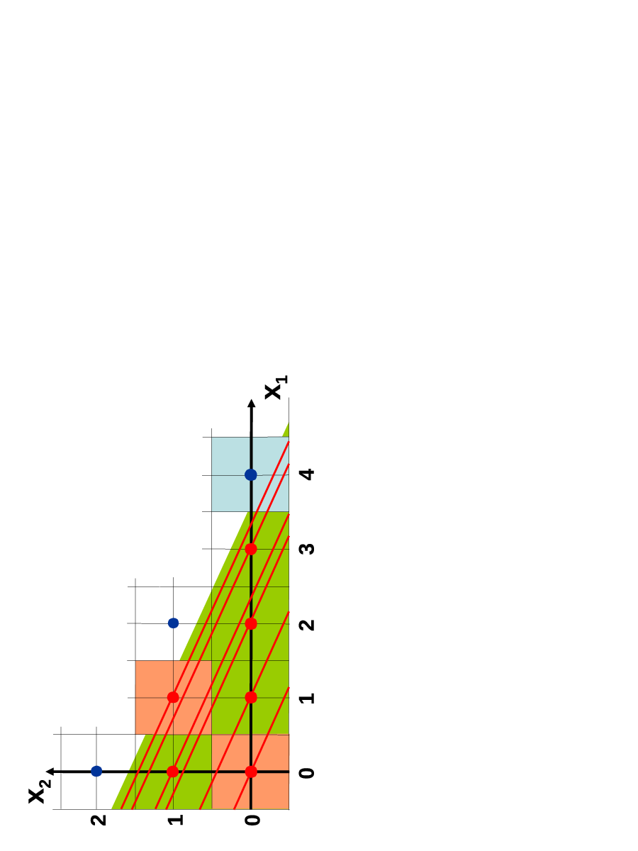
and both and greater than minus 1/2. This triangular domain is represented in Fig. 1 for , and kept at 5.2, 1 and 2.3 respectively ; these values have been chosen in such a way that six quantum states, indicated by red dots, are available (different values might have been chosen as well). Three forbidden quantum states are represented by dark blue dots and three unit squares centered on quantum states are emphasized. The two salmon ones correspond to available quantum states while the light blue one corresponds to a forbidden state.
Throughout the present part, will be simply denoted . Its value is
| (18) |
(the inverse of the area of the green triangle) inside the triangle and zero outside.
can be determined analytically by using the identity
| (19) |
leading to
| (20) |
Additional paragraph 4:
In principle, the translational energy distribution measured in a perfect experiment would consist in
a set of Dirac delta functions for the energies complementary with those of the allowed product quantum
states. However, no experiment is "perfect". There is always an uncertainty in both the total energy
available to the products and the measure of the translational energy. Consequently, the peaks are
necessarily broaden.
In order to take into account
this uncertainty in the theory, we shall replace the Dirac peaks present in Eqs. (9), (11) and (16)
by (see Eq. (2)) with , meaning that the uncertainty on is 0.1.
This arbitrary value of makes the peaks neither too narrow, nor too broad as compared to the total
energy . The fact that it was kept at the same value as in the GB procedure should not confuse the reader.
Its choice was a matter of convenience, nothing else.
It is worth emphasizing that there are thus two separate issues in this work: the first, and central one, is the use of Gaussians
to deal with Bohr quantization in QCT calculations ; the second, and minor one, is the use of Gaussians
to take into account the uncertainty in the measurement of the translational energy.
End of the additional paragraph 4.
and were determined by Monte-Carlo integration over and ,
using points randomly chosen in the triangular domain.
The corresponding expressions are
| (21) |
where stands for or , with
| (22) |
being the number of trajectories ending in , and
| (23) |
and being the final actions for the trajectory ending in .
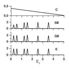
The four distributions are represented in Fig. 2 for 500 values of regularly distributed between 0 and .
appears to be in complete disagreement with the "benchmark" distribution , for by construction, no structure can be reproduced. takes the structures into account, but the heights of the peaks are inaccurate for the small values of . Conversely, is in excellent agreement with , as expected. Note that for these two distributions, the peaks have the same height, meaning that the populations of the available quantum states are all equal, in agreement with the statistical hypothesis.
The heights of the peaks of increase with . This can be easily understood from Fig. 1.
The values of the translational energies corresponding to the top of
the peaks (see Fig. 2) are given by
| (24) |
the integers an being such that is an allowed quantum state. These states are , ,
, , and , by order of increasing translational energy.
The straight lines defined by
| (25) |
are represented in Fig. 1. Clearly, the spacings between these lines exactly follow the spacings between the nearest ’s (see Fig. 2).
Now, the heights are proportional to the SB populations, themselves proportional to the available areas of the unit squares centered on the quantum states. From Fig. 1, it is clear that for , this area, represented in salmon, is 1, but for , it is only equal to 0.6. One also guesses that for and , the areas are equal to 0.7 and 0.9 respectively while for the remaining states and , they are equal to 1. This explains why the heights of the first three peaks of (see Fig. 2) are only 60, 70 and 90 percent of the height of the remaining peaks. This cannot happen with the GB distribution, for with sufficiently thin Gaussians, their value is the same for all the quantum states.
Having defined the system of interest and applied the different methods currently utilized in QCT calculations today,
we are now in a position to introduce the 1GB procedure. ,
given by Eq. (14) with , can be rewritten as
| (26) |
where and are two new coordinates related to and by the rotation
| (27) |
and
| (28) |
with
| (29) |
and
| (30) |
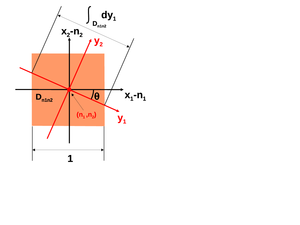
The axis runs through and is parallel to the hypotenuse of the green triangle. is thus one of the red axes represented in Fig. 1. The axis also runs through and is orthogonal to . These axes are represented in Fig. 3 as well as the unit square . It is clear that integration over and in Eq. (26) immediately leads to Eq. (15).
Let us now define the population
| (31) |
where
| (32) |
As compared with Eq. (26), Eq. (31) involves only one Dirac distribution. After a trivial integration
with respect to , reads
| (33) |
However, one deduces from Fig. 3, corresponding to the case where is greater than
( lower than ), that
| (34) |
In the same way, it can be easily shown that when is smaller than ,
| (35) |
, given by Eq. (32), can thus be rewritten as
| (36) |
and Eq. (33) leads to
| (37) |
We thus arrive at the conclusion that the ’s are equal to the ’s (see Eq. (15)).
Consequently, can be rewritten from Eqs. (28)-(31) as
| (38) |
Moreover, from Eqs. (29), (30) and (32) and using the fact that
(deduced from Eq. (19)), we obtain
| (39) |
Applying the GB procedure, i.e. replacing by , and going back to the ’s,
finally reads
| (40) |
an expression formally close to the expression
| (41) |
corresponding to the calculations of Czakó and Bowman [37].
is then deduced from by
| (42) |
Like previously, the function in the above expression is replaced by a Gaussian in order to take into account
the uncertainty in the measurement of the translational energy. Moreover, the Monte-Carlo expression of reads
| (43) |
with
| (44) |
according to Eq. (40) or
| (45) |
according to Eq. (41). Eqs. (2), (43) and (45) correspond to
Eqs. 13 and 16 in the paper by Czakó and Bowman [37].
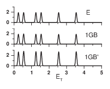
The distribution obtained from Eqs. (42)-(44) is represented in Fig. 4 (1GB curve),
together with (like previously, was kept at 0.05 for all the Gaussians).
The two densities are in such a good agreement that they cannot be distinguished.
On the other hand, the distribution obtained from Eqs. (42), (43) and (45), also shown in
Fig. 4 (1GB’ curve), has the good shape, but its norm is too large. We shall come back to this
important normalization issue in section II.H.
Additional paragraph 5:
One may wonder wether the selection of to be the argument of the delta function in Eq. (31) is arbitrary.
For instance, one might be tempted by stating in view of Fig. 3 that interchanging and still
leads to the equality between and . This is indeed true for the less excited states
, , and , but not for the most excited states and (see Fig. 1). As a matter
of fact, the upper limit of the green triangle would limit the integration along the new axis (corresponding to the axis
in Fig. 3) in such a way
that for and , would be lower than .
On the other hand, slightly varying about
the value defined by Eqs. (29) and (30) will preserve the equality between and
provided that the hypotenuse of the green triangle is not too close to the most excited states.
Strictly speaking, the value of defined by Eqs. (29) and (30) is thus not the only
satisfying one. Nevertheless, it is the only one for which the equality between and
is systematically satisfied, no matter how close to the most excited states the hypotenuse is.
This makes it superior to any other one.
End of additional paragraph 5.
II.5.2 Non statistical case
What about non statistical situations ? Given that is non uniform in the energetically allowed triangle,
Eq. (33) reads
| (46) |
Recall that in the statistical case, the 1GB procedure was justified by the fact that is equal to .
In the present case, is still a reasonable approximation of provided that
the variation of along the -axis is sufficiently smooth. If so, it is indeed clear using Eq. (36) that
| (47) |
the strict equality occuring when varies linearly along the -axis (and is non zero within ). From Eq. (15), we then arrive at the conclusion that is roughly equal to .
Such a smooth variation of the density in the action space
was observed several times in the case of three-atom exchange reactions, the only difference
being that the previously introduced and actions play the role of and . Fig. 4 in reference
[20] is a clear illustration of this statement in the case of the direct
reaction O(3P)+HCl OH+Cl(2P).
The energetically available area in the
plane is given by
| (48) |
Its upper limit is thus found to be a curved, instead of straight, line. Moreover, the lines equivalent to the six straight lines in Fig. 1 are also curved. Along these lines (not drawn in Fig. 4 of reference [20]), the density evolves rather smoothly. In other words, despite the fact that the distribution of the translational energy is not statistical, the intra-molecular vibrational redistribution (IVR) in the strong coupling region tends to distribute in a relatively democratic way the rest of the energy among the vibrational and rotational degrees-of-freedom.
One expects a similar redistribution will also take place among the vibrational modes, due to their couplings. As shown in section IV, this is at least the case for OH+D2 which, as O(3P)+HCl, is a direct process.
II.6 Collisional system involving three vibrational modes
We now consider the collinear inelastic collision between atom A and the tetra-atomic molecule BCDE involving three vibrational
normal modes. Following a reasoning analogous to the one developed in the previous subsection, we arrived after some steps of algebra to
an expression exact (with a Gaussian of zero width) in the statistical limit ( being still considered as the "exact" density). With
, , the unit cube centered on , and
, and deduced from any cyclic permutation
of , and , this expression is
| (49) |
with
| (50) |
being defined as
| (51) |
if for the three cyclic permutations, or
| (52) |
if for only one of the permutations. In the second case, the formulation (see Eqs. (50) and (52)) is a straightforward extension of Eq. (40).
We shall retain from the above developments that for three vibrational modes, the formulation of is not unique. It depends on the values of the vibrational frequencies , and , contrary to the formulation for two vibrational modes.
Hence, if one does not use the correct expression of , one does not find the correct populations. However, the wrong populations turn out to be proportional to the correct ones. The proof is straightforward: if we call the correct value of and the wrong one, the wrong populations are found from Eqs. (50) (with replaced by the Dirac distribution) and (19) to be equal to times the correct populations. This explains why the peaks of the 1GB’ distribution in Fig. 4 (given by Eqs. (41) and (42)) are higher than the peaks of the 1GB distribution (given by Eqs. (40) and (42)).
We did not extend the above developments in the case of systems involving more than three vibrational modes for the mathematical developments became very tedious. Therefore, we do not know the analytical expression of making the 1GB distribution in close agreement with the "exact" or GB distribution in the statistical limit. However, we go round this difficulty in section II.H.
II.7 General collisions
The extension of Eq. (6) to a three-dimensional collision involving vibrational modes is
| (53) |
where
| (54) |
, is the final product rotational energy and is the distribution of and .
For a given value of , appears to be formally identical to in Eq. (6)
and consequently, all the developments following Eq. (6) could be repeated here identically.
The main conclusion of this section is thus the same as before, i.e., the 1GB procedure
leads to nearly the same conclusions as the GB procedure provided that
the variation of in any plane parallel to the plane
| (55) |
is sufficiently smooth. As stated before, however, we do not know the expressions analogous to Eq. (40) and Eqs. (50)-(52) for larger than 3.
II.8 Normalization procedure in realistic calculations
The Monte-Carlo expression of the
1GB populations of the final product quantum states is given by
| (56) |
where is the total number of trajectories run and is the number of trajectories ending in the product channel with pointing in , the -dimensional unit cube centered on .
As seen before, however, we do not know in the general case the expression of leading to 1GB distributions in close agreement with the GB ones in the statistical limit. Nevertheless, the former are proportional to the latter.
One might thus think about re-normalizing 1GB distributions so as to give them the GB norms. But
GB norms have no reason to be exactly equal to one,
so it is preferable to directly re-normalize 1GB distributions to unity. The corresponding
expression is
| (57) |
where may be kept at the maximum of the frequencies or their sum. The final result is not expected to depend significantly on this choice, for it will affect both the numerator and the denominator of Eq. (57) in nearly the same way. This point is illustrated in section IV in the case of the reaction OH + D2. Note that in the denominator, the sum is over the whole set of computed trajectories, be they reactive or not. The various quantities in the argument of the Gaussian are thus either those of the products and those of the reformed reagents.
Special care should however be taken with processes
involving a large amount of vibrationally elastic non reactive trajectories. Ion-molecule reactions are
a typical example. For such processes, an alternative to Eq. (57) is
| (58) |
where the sum over in the denominator involves the whole set of final vibrational states, i.e., those of the products as well as those of the reformed reactants. Eq. (58) is a compact form of Eqs. (15) and (16) of reference 23. Eq. (4) of reference 34 may be a second alternative.
III Non statistical test case for three vibrational modes
We still consider the collinear inelastic collision between atom A and the tetra-atomic molecule BCDE involving three harmonic
normal modes. , , and are respectively kept at 15, 1, 1.7 and 2.9.
We also consider the non statistical Gaussian density given by
| (59) |
with , and , being kept at in , in and in .
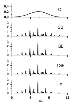
The resulting distributions , , , and , given by expressions similar to those of the previous section with one more dimension, are represented in Fig. 5. The details of the calculations are exactly the same as in section II.D.1, the only difference being that all the distributions were numerically re-normalized to unity.
Like in the previous statistical example, is in poor agreement with . On the other hand, is in very good agreement with ; given the large number of points considered in the Monte-Carlo integration, this is an expected result despite the already "large" number of vibrational modes involved in the collision.
Interestingly, is even in slightly better accord with than when looking at the details. Such a high level of agreement despite the non-statistical nature of the present process is pleasing. It supports the statement of subsection II.E.2 that for a sufficiently smooth distribution of the final actions, the 1GB procedure represents an accurate alternative to the GB one.
Last but not least, does also a good job, though the heights of the peaks corresponding to the largest energies tend to be overestimated.
IV The simplest polyatomic reaction OH+D2 HOD+D
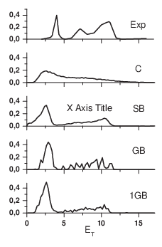
This process has been the subject of intense research, both experimentally and theoretically [38, 39, 40, 41, 42, 43, 44, 51]. Its mechanism has been well established as being direct, with the products preferentially backward scattered, suggestive of a rebound mechanism. The product translational energy distribution was experimentally measured by Alagia et al. [38], and by Davis and co-workers four years later [40]. While Alagia et al. found a broad and single-peaked distribution, Davis et al. found a better resolved distribution involving three peaks corresponding to the HOD vibrational states = (0,1,0), (0,2,0) and (0,1,1). , and are the OH stretching, bending and OD stretching quantum numbers, respectively. This distribution is represented in the top panel of Fig. 6.
In reference 41, 1 000 000 trajectories were run on the Ochoa-Clary (OC) potential energy surface (PES) [51] using the VENUS96 code. Initial conditions were selected to reproduce the experiment of Davis and co-workers, with a collision energy of 6.6 kcal mol-1 and the reactants in their vibrational ground states. The number of reactive trajectories was found equal to . At the end of each reactive trajectory, the vibrational actions of the triatomic HOD product were calculated using the recent normal mode analysis algorithm [52]. The latter includes anharmonicity and Coriolis-coupling terms, and yields results similar to those obtained by means of the widely used fast Fourier transform approach [53], but at a lower computational cost.
The different distributions previously considered are calculated as follows.
Formally, the purely classical translational energy distribution is given by
Eqs. (53) and (54) with equal 3.
Stricto-sensu, its Monte-Carlo expression is
| (60) |
where is the final translational energy for the trajectory. This energy satisfies the relation
| (61) |
the ’s and being the final vibrational actions and rotational energy for the trajectory.
Here, we shall not replace the Dirac distribution in the previous sum by a Gaussian and calculate it for fixed values
of . Instead, we divide the available range of energy in boxes ,
, and integrate over the boxes. This leads to the populations
| (62) |
, where is the number of trajectories for which the final translational energy belongs to the box.
We note that applying Eq. (60) does only require the calculation of , not of , , and .
On the other hand, the four last quantities are necessary for the calculation of . This distribution is indeed calculated
in the same way as , the only difference being that the translational energy for the trajectory is now given by
| (63) |
instead of Eq. (61). This difference is similar to the one between Eqs. (6) and (7).
For , is replaced in Eq. (62) by
| (64) |
the sum being performed over the trajectories for which the final translational energy according to Eq. (61) belongs to the box.
For , is replaced by
| (65) |
the sum being performed over the same trajectories as above.
Finally, , and were re-normalized to one. was kept at 0.05 for , and 0.01 for . was identified with the largest frequency. The distributions are displayed in Fig. 6. We also kept at the sum of the frequencies, following Czako and Bowman [37], but due to the re-normalization, this left the distribution unchanged.
Contrary to the purely classical distribution which has a bell shape and does not reproduce the vibrational structures observed experimentally [43, 44], the SB, GB and 1GB distributions reproduce quite satisfyingly the two structures due to the (0,1,0) and (0,2,0) vibrational states. On the other hand, the third structure, due to the (0,1,1) state, is strongly underestimated by all the treatments. Comparison with exact quantum scattering calculations, certainly possible in a near future, will tell if the previous disagreement is due to possible inaccuracies of the OC-PES or to the present classical descriptions.
The SB procedure does a good job, though it overestimates the contribution of the small translational energies to the (0,2,0) peak.
The GB distribution of Fig. 6 involves strong fluctuations, contrary to the same density represented in Fig. 2 of reference 41. The reason is that in the present work, we did not use the smoothing procedure previously considered [44] (two Gaussian functions were used to fit the left and right-hand side of each vibrational contribution). We did it on purpose, in order to illustrate the fact that with 11000 reactive trajectories and three vibrational modes, the usual GB procedure generates quite noisy curves. On the other hand, the 1GB distribution is much better converged and one guesses that it represents the curve one would obtain from smoothing the GB curve.
Owing to the fact that the OH+D2 reaction is a direct process, the present results are quite encouraging for future applications of the 1GB procedure to polyatomic reactions, do they involve a long-lived complex or not.
V Conclusion
In the recent years, many processes have been studied by the quasi-classical trajectory method (QCTM) within
the Gaussian binning (GB) procedure. In most studies, the population of the final product quantum state
, being the number of quantized degrees of freedom (DOF), was approximated by
| (66) |
instead of the usual expression
| (67) |
used in the standard binning (SB) procedure (or histogram method). is the total number of trajectories run, is the final action state, is the number of trajectories ending in the product channel with pointing in the -dimensional unit cube centered on and is a Gaussian normalized to unity, with a full width at half maximum of 10 percent.
Since most processes studied so far by GB-QCTM were triatomic reactions, one single vibrational DOF was quantized, meaning that the Gaussian product in Eq. (66) reduced to one term only. As about 10 percent of the total amount of reactive trajectories do actually contribute to the product populations, 10 times more trajectories had to be run for keeping with the same level of convergence of the predictions as compared with SB-QCTM.
Nowadays, however, more and more processes under scrutiny involve more than one vibrational mode. For instance, the reaction OH+D HOD+D involves three modes while for the reaction F+CH FH+CH3, this number is seven. Consequently, GB-QCTM requires one thousand more trajectories than SB-QCTM for the first process and ten millions more for the second ! It is thus quite clear that as such, Eq. (66) has no future in the area of polyatomic reaction dynamics.
This is why Czakó and Bowman [37] recently proposed to "quantize" the total vibrational energy
instead of the vibrational actions, introducing the expression
| (68) |
where is the normal mode frequency and
| (69) |
The key feature of this ad-hoc quantization as compared to the previous one-Gaussian-for-one-mode approach is that only one Gaussian function is used whatever the number of vibrational DOF of the system, a huge amount of computational time being therefore saved. We called it the 1GB procedure.
The conclusions of the present paper are as follows:
1) For a statistical collision involving two product vibrational modes, the 1GB procedure
is strictly equivalent to the GB procedure provided that is identified with the maximum of the
’s instead of their sum.
2) For a statistical collision involving three product vibrational modes, the 1GB procedure
is strictly equivalent to the GB procedure provided that is kept at the maximum frequency in part
of the frequency space, and a more complex expression (see Eq. (51)) in the remaining part.
3) For the previous processes and a non statistical but sufficiently smooth distribution in the action space,
the 1GB procedure leads to results in satisfying agreement with the GB ones.
4) Finding the expression of for any realistic process involving more than
three product vibrational modes requires heavy mathematical developments that we did not perform. However,
one may go round this difficulty by re-normalizing the product state populations. In such a case, can be indifferently
kept at the maximum of the ’s or their sum. Special care should however be taken with processes
involving a large amount of vibrationally elastic non reactive trajectories, like ion-molecule reactions.
The methods proposed in reference 23 (leading to Eq. (58) of the present work) or 34 can then be used.
5) The 1GB procedure leads to results in good agreement with the GB one for (a) a non statistical test case
involving three vibrational modes and (b) the prototype four-atom reaction OH+D2 HOD+D.
In conclusion, the 1GB procedure might be of great interest for future classical simulations of polyatomic chemical
reaction dynamics in the highly quantum mechanical situation where only a few product vibrational states are
available.
Appendix
Consider (i) the -dimensional space , (ii) a given distribution , normalized to unity, of the position in the previous space and (iii) the quantity depending on according to
| (B.1) |
The probability that is lower than a given value is given by
| (B.2) |
where is the Heaviside function, equal to 0 for negative and 1 in the contrary case. ensures that integration with respect to is made over the volume such that minus is positive, i.e., is lower than .
If is the density of probability that takes the value , is the probability that
belongs to the range [, ]. We then have
| (B.3) |
that is,
| (B.4) |
From Eq. (B.2), we finally arrive at
| (B.5) |
as the Dirac distribution is the first derivative of . Eq. (6) is straightforwardly obtained from Eqs. (B.5), (4) and (5).
Acknowledgments
LB is endebted to Pr. J.-C. Rayez for careful reading of the manuscript prior to its publication as well as stimulating discussions on its content and more generally, on the semi-classical description of molecular collisions.
References
- [1] R. Levine, Molecular Reaction Dynamics, Cambridge University Press, 2005.
- [2] See, among many others, I. N. Levine, Quantum Chemistry, 6th Edition, Prentice Hall, 2008 ; F. L. Pilar, Elementary Quantum Chemistry, Second Edition, Dover Publications, 2001 ; T. Helgaker, P. Jorgensen and J. Olsen, Molecular Electronic Structure Theory, Wiley, 2000.
- [3] P. Honvault and J.-M. Launay in Theory of Chemical Reaction Dynamics, Kluwer Academic Publishers, 2004.
- [4] V. Aquilanti and S. Tonzani, J. Chem. Phys., 120, 4066 (2004).
- [5] G. Nyman and H.-G. Yu, Rep. Prog. Phys., 63, 1001 (2000).
- [6] S. Althorpe in The Encyclopedia of Computational Chemistry, Ed. P. Schleyer, Wiley, Athens, 2005.
- [7] W. Hu and G. C. Schatz, J. Chem. Phys., 125, 132301 (2006).
- [8] B. Lepetit, D. Wang and A. Kuppermann, J. Chem. Phys., 125, 133505 (2006).
- [9] X.Q. Zhang, Q. Cui, J.Z.H. Zhang, K.L. Han, J. Chem. Phys., 126, 234304 (2007).
- [10] D. De Fazio, V. Aquilanti, S. Cavalli, A. Aguilar and J. M. Lucas, J. Chem. Phys., 129, 064303 (2008).
- [11] R. N. Porter and L. M. Raff, in Dynamics of molecular collisions, Part B, edited by W. H. Miller, Plenum, New York, 1976.
- [12] T. D. Sewell and D. L. Thomson, Int. J. Mod. Phys. B, 11, 1067 (1997).
- [13] D. Clary, Phys. Chem. Chem. Phys., 9, pp.C21 (2007) and references therein.
- [14] M. Ragni, A. C. P. Bitencourt and V. Aquilanti, Int. J. Quant. Chem., 107, 2870 (2007).
- [15] B. Lepetit, D. Wang and A. Kuppermann, J. Chem. Phys., 125, 133505 (2006).
- [16] S. Schmatz, ChemPhysChem, 5, 600 (2004).
- [17] M. Yang, S-Y. Lee, and D. H. Zhang J. Chem. Phys., 126, 064303 (2007).
- [18] L. Bonnet and J.-C. Rayez, Chem. Phys. Lett., 277, 183 (1997).
- [19] L. Bañares, F. J. Aoiz, P. Honvault, B. Bussery-Honvault and J.-M. Launay, J. Chem. Phys., 118, 565 (2003).
- [20] T. Xie, J. Bowman, J. W. Duff, M. Braunstein and B. Ramachandran J. Chem. Phys., 122, 014301 (2005).
- [21] M. L. González-Martinez, L. Bonnet, P. Larrégaray and J.-C. Rayez, J. Chem. Phys., 126, 041102 (2007).
- [22] S. Ron, M. Baer and E. Pollak, J. Chem. Phys., 78, 4414 (1983).
- [23] L. Bonnet and J.-C. Rayez, Chem. Phys. Lett., 397, 106 (2004).
- [24] L. Bonnet, J. Chem. Phys., 128, 044109 (2008).
- [25] W. H. Miller, J. Chem. Phys., 53, 1949 (1970).
- [26] R. A. Marcus, Chem. Phys. Lett., 7, 252 (1970).
- [27] W. H. Miller, Adv. Chem. Phys., 25, 69 (1974).
- [28] W. H. Miller, J. Phys. Chem. A, 105, 2942 (2001).
- [29] M. S. Child, Molecular Collision Theory, 1974 (Academic Press).
- [30] J. N. L. Connor, Chem. Soc. Rev., 5, 125 (1976).
- [31] L. Bonnet and C. Crespos, Phys. Rev. A, 78, 062713 (2008).
- [32] Z. Sun, D. H. Zhang, C. Xu, S. Zhou, D. Xie, G. Lendvay, S-Y. Lee, S. Y. Lin, and H. Guo, J. Am. Chem. Soc., 130, 14962 (2008).
- [33] G. Lendvay, D. Xie and H. Guo, Chem. Phys., 349, 181 (2008).
- [34] P. Halvick, T. Stoecklin, P. Larrégaray and L. Bonnet, Phys. Chem. Chem. Phys., 9, 582 (2007).
- [35] Z. Sun, L. Liu, S.Y. Lin, R. Schinke, H. Guo, D.H. Zhang, Proc. Nat. Acad. Sci., 107, 555 (2010).
- [36] K. Liu, Phys. Chem. Chem. Phys., 9, 17 (2007).
- [37] G. Czakó and J. M. Bowman, J. Chem. Phys., 131, 244302 (2009).
- [38] M. Alagia, N. Balucani, P. Casavecchia, D. Stranges, G. G. Volpi, D. C. Clary, A. Kliesch and H.-J. Warner, Chem. Phys., 207, 389 (1996).
- [39] S. K. Pogrebnya, J. Palma, D. C. Clary and J. Echave, Phys. Chem. Chem. Phys., 2000, 2, 693, Phys. Chem. Chem. Phys., 2, 693 (2000).
- [40] B. R. Strazisar, C. Lin and H. F. Davis, Science, 290, 958 (2000).
- [41] J. D. Sierra, P. A. Enriquez, D. Troya and M. Gonzalez, Chem. Phys. Lett., 399, 527 (2004).
- [42] E. Garcia, A. Saracibar, A. Rodríguez, A. Lagana and G. Lendvay, Mol. Phys., 2006, 104, 839 Mol. Phys., 104, 839 (2006).
- [43] J. D. Sierra, R. Martínez, J. Hernando and M. González, Phys. Chem. Chem. Phys., 11, 11520 (2009).
- [44] J. Espinosa-Garcia, L. Bonnet and J. C. Corchado, Phys. Chem. Chem. Phys., 12, 3873 (2010).
- [45] L. Bonnet and J.-C. Rayez, J. Phys. Chem. A, 101, 9318 (1997).
- [46] P. Larrégaray, L. Bonnet and J.-C. Rayez, J. Phys. Chem. A, 110, 1552 (2006).
- [47] L. Bonnet, P. Larrégaray, J.-C. Rayez and T. Gonzalez-Lezana, Phys. Chem. Chem. Phys., 8, 3951 (2006).
- [48] T. González-Lezana, Int. Rev. Phys. Chem., 26, 29 (2007).
- [49] F. J. Aoiz, V. S Rábanos, T. González-Lezana and D. E. Manolopoulos, J. Chem. Phys., 126, 161101 (2007).
- [50] L. Bonnet, P. Larrégaray and J.-C. Rayez, Phys. Chem. Chem. Phys., 9, 3228 (2007).
- [51] G. Ochoa de Aspuru and D. Clary, J. Phys. Chem. A, 102, 9631 (1998)
- [52] J. C. Corchado and J. Espinosa-Garcia, Phys. Chem. Chem. Phys., 11, 10157 (2009).
- [53] G. C. Schatz, Comput. Phys. Commun., 51, 135 (1988).
Figures captions
Fig. 1: The action space defined by Eq. (17)
and both and greater than minus 1/2 is represented here by a green triangle while the available quantum states
are represented by six red dots. The distribution of the action pair
is uniform in the triangle. Each dot lies along a straight-line corresponding
to a given translational energy (see Eq. (25)).
Three forbidden quantum states are represented by dark blue dots and
three unit squares centered on quantum states are emphasized. The two salmon ones
correspond to available quantum states while the light blue one corresponds to
a forbidden state.
Fig. 2: Translational energy distributions corresponding to the
statistical distribution in the green triangle of Fig. 1.
The curves are labeled by the subscript of their mathematical
symbols (see text). The distributions are not normalized to unity.
Fig. 3: Drawing shedding light on the derivation of
Eq. (40). clearly appears to be the reciprocal of
the section of the new coordinate axis being within the red square
(see Eq. (34)).
Fig. 4: Translational energy distributions corresponding to the
statistical distribution in the green triangle of Fig. 1.
The curves are labeled by the subscript of their mathematical
symbols (see text). The distributions are not normalized to unity.
Fig. 5: Translational energy distributions corresponding to the
non statistical distribution given by Eq. (59).
The curves are labeled by the subscript of their mathematical
symbols (see text). The distributions are not normalized to unity.
Fig. 6: Translational energy distributions in the products
of the reaction OH+D2 HOD+D studied at the conditions
of the group of Davis [40]. The top curve is the
experimental distribution while the remaining curves are labeled by
the subscript of their mathematical symbols (see text).
The distributions are normalized to unity.
Figures