Robustness of Majorana Modes and Minigaps in a Spin-Orbit-Coupled Semiconductor-Superconductor Heterostructure
Abstract
We study the robustness of Majorana zero energy modes and minigaps of quasiparticle excitations in a vortex by numerically solving Bogoliubov-deGennes equations in a heterostructure composed of an s-wave superconductor, a spin-orbit-coupled semiconductor thin film, and a magnetic insulator. This heterostructure was proposed recently as a platform for observing non-Abelian statistics and performing topological quantum computation. The dependence of the Majorana zero energy states and the minigaps on various physics parameters (Zeeman field, chemical potential, spin-orbit coupling strength) is characterized. We find the minigaps depend strongly on the spin-orbit coupling strength. In certain parameter region, the minigaps are linearly proportional to the s-wave superconducting pairing gap , which is very different from the dependence in a regular s- or p-wave superconductor. We characterize the zero energy chiral edge state at the boundary and calculate the STM signal in the vortex core that shows a pronounced zero energy peak. We show that the Majorana zero energy states are robust in the presence of various types of impurities. We find the existence of impurity potential may increase the minigaps and thus benefit topological quantum computation.
pacs
03.67.Lx, 71.10.Pm, 74.45.+cI Introduction
Topological quantum computation (TQC) [1, 2], where quantum information is processed using a decoherence-free subspace guaranteed by topological order, is a revolutionary new alternative to conventional quantum computing. In TQC, quantum information is encoded in certain nonlocal, topological, degrees of freedom of the underlying physical system (i.e., hardware) that do not couple to weak local noise. This special hardware, called ’non-Abelian topological matter’, has been proposed to exist in certain classes of two-dimensional (2D) strongly-correlated systems, such as the fractional quantum Hall (FQH) system [3, 4, 5, 6, 7, 8, 9], chiral p-wave superconductor/superfluid [10, 11, 12, 13, 14, 15, 16, 17, 18, 19, 20], and some artificial states of cold atoms in optical lattices [21, 22, 23]. In these systems, the ground state wave function is a linear combination of states from a degenerate subspace, and a pair-wise exchange of the particle coordinates unitarily rotates the ground state wave function in this subspace. Therefore, the exchange statistics of the particles is given by a multi-dimensional unitary matrix representation (as opposed to just a phase factor for bosons and fermions) of the 2D braid group, and the statistics is non-Abelian.
Despite the tremendous technological potential, non-Abelian topological matter is rare in nature and generally hard to observe in experiments [1]. To circumvent this problem, there has been considerable interests recently for exploring the possibility of ‘designing’ non-Abelian topological order in the fertile laboratory of the cold atom systems [24, 25] and the regular solid state materials [26, 27, 28, 29, 30, 31, 32, 33, 34, 35, 36, 37, 38, 39, 40]. Two important resources for the emergence of non-Abelian statistics in a correlated matter are (a) chirality of the constituent particles and (b) superconducting order. In a composite system, these two basic ingredients of topological order may arise from two different physical effects (for instance, spin-orbit coupling and s-wave superconductivity, respectively) to design a non-Abelian quantum state. This strategy allows us to use s-wave superconductors/superfluids, which are much more abundant in nature and much less sensitive to disorder effects than their p-wave counterparts.
One important recent progress along this direction was the proposed solid state heterostructure composed of an electron-doped semiconductor thin film, an s-wave superconductor, and a magnetic insulator as a non-Abelian platform for TQC [30]. In this heterostructure, the superconducting pairing order is induced on the semiconductor thin film from the s-wave superconductor through the superconducting proximity effect, and the chirality of particles is supplied by the Rashba spin-orbit coupling in the semiconductor [41]. With a set of vortices in the heterostructure, there exist one Majorana zero energy state of quasiparticle excitations in each vortex core. These zero energy states are the topological, degenerate, ground states following non-Abelian statistics and can be used to perform TQC.
In addition to the existence of Majorana zero energy modes, another key ingredient for the physical implementation of TQC is that the degenerate ground state subspace must be separated from other non-topological excited states by an energy gap, so that finite temperature cannot populate the excited states and ruin the topological properties of the system. Recently, it was shown[42], by constructing a new type of Majorana operators that contain both zero energy and excited states, that the topological braiding statistics of Majorana fermions may still preserve even in the presence of non-topological excitations. However, the minigap is still important because the signal strengths of measurements will be reduced significantly when the temperature is comparable with the minigap where the number of non-topological excitations become significant. The magnitude of the energy gap directly determines the operating temperature of the underlying physical system as a realistic TQC platform and is of critical importance. Furthermore, both Majorana zero energy states and the magnitude of the gap must be robust in the presence of various impurities. Although the existence of Majorana zero energy states in the vortex core in a heterostructure has been proved by analyzing the zero energy solution of the Bogoliubov-deGennes (BdG) equation, the magnitudes of the minimum energy gaps and their robustness against impurities have not been addressed.
In this paper, we numerically solve the BdG equation for a vortex in the heterostructure and calculate the minimum energy gap (minigap) between the zero energy state and the first quasiparticle excited state in the vortex core. In the simulation, the proximity-induced -wave superconducting pairing gap in the semiconductor is obtained from the self-consistent solution of the BdG equations for a pure -wave superconductor. The main results are summarized as follows:
1) The full numerical simulation of the BdG equations confirms that the Majorana zero energy states exist only in the parameter region , which agrees with previous results obtained from an approximate analytical approach. Here is the perpendicular Zeeman field induced by the proximity contact with the magnetic insulator, is the chemical potential of the electron gas.
2) The dependence of the minigap on various parameters is characterized. Here is the strength of the Rashba spin-orbit coupling in the semiconductor. We find depends strongly on . In certain parameter region, is , instead of for a regular chiral -wave superconductor/superfluid [43].
3) An analytical theory is developed to explain the properties of the zero energy chiral edge states at the boundary.
4) The scanning tunneling microscopy (STM) signals around the vortex show pronounced peaks at the zero energy and the minigap, thus can be used to detect the zero energy modes and the minigaps in experiments.
5) We show that Majorana zero energy modes are robust in the presence of various impurity potentials. Surprisingly, we find the existence of impurity potential in the vortex core may increase the magnitudes of the minigaps, and thus may be useful for the physical implementation of TQC.
The paper is organized as follows: Section II lays out the BdG equation for a vortex in a semiconductor-superconductor heterostructure. Section III discusses the parameter dependence of the zero energy states and the minigap . In Sec. IV, we discuss the robustness of the zero energy states and the minigaps in the presence of realistic impurities. Section V consists of conclusions. The details about the numerical approach to the BdG equations are presented in Appendix A. The finite size effect in the BdG equations is discussed in Appendix B. In Appendix C, we discuss the zero energy chiral edge modes at the boundary.
II BdG equations for a vortex
The physical system we consider is a heterostructure composed of an s-wave superconductor, an electron-doped semiconductor thin film, and a magnetic insulator (Fig. 1a). The dynamics of electrons in the semiconductor are described by a single particle effective Hamiltonian
| (1) |
where is the conduction-band effective mass of electrons, is the chemical potential, is the strength of the Rashba spin-orbit coupling, is a perpendicular Zeeman field induced by the proximity contact with the magnetic insulator. are the Pauli matrices for the electron spins.
The Hamiltonian yields two spin-orbit bands (Fig. 1b) with energy dispersions
| (2) |
in a uniform system. Henceforth we set . A finite energy gap is opened at for a nonzero . When the chemical potential lays in the gap, electrons only occupy the lower spin-orbit band at a low temperature.

The mean field Hamiltonian of an -wave superconductor can be written as
| (3) |
in the Nambu space, where is the single particle Hamiltonian, is Fermi energy, is an external potential, are annihilation operators of electrons for position eigenfunctions rather than for momentum eigenfunctions, is the s-wave pairing order parameter. The Hamiltonian (3) can be diagonalized by the Bogoliubov transformation
| (4) |
where the wavefunctions , satisfy the BdG equation
| (5) |
and the normalization condition
| (6) |
The order parameter can be determined self-consistently[44] through the relation . Here is the effective electron-electron interaction strength in the superconductor.
The proximity effect between the s-wave superconductor and the semiconductor induces an effective superconducting pairing for electrons in the semiconductor described by the Hamiltonian
| (7) |
where are the creation operators for electrons, and is the proximity-induced effective s-wave pairing gap in the semiconductor thin film. Because of the Rashba spin-orbit coupling in the semiconductor, the single particle Hamiltonian in the BdG equation (5) should now be replaced with in (1). The BdG equation written in the Nambu spinor basis becomes
| (8) |
where is the quasiparticle wavefunction. The Bogoliubov quasiparticle operator is
| (9) |

In the presence of a vortex in the semiconductor-superconductor heterostructure, the order parameter takes the form , and the solutions of the BdG equation (8) correspond to the quasiparticle excitation energies and states in the vortex core. For simplicity of the calculation, we consider a two-dimensional cylinder geometry with a hard wall at the radius and a single vortex at . This system preserves the rotation symmetry and the BdG equation can be decoupled into different angular momentum channels indexed by with the corresponding spinor wavefunction
| (10) |
Note that the BdG equation has the particle-hole symmetry, therefore if is a solution with an energy , then there is another solution with the energy in the angular momentum channel. Henceforth we only consider solutions.
III Majorana modes and minigaps
We numerically solve the BdG equation (8) with a vortex and calculate the quasiparticle excitation energy and wavefunction for various parameters . In the numerical treatment, the radial wave functions in Eq. (10) are expanded on an orthogonal basis , where is the -th order Bessel function, is the -th zero of . This basis satisfies the boundary condition automatically. The BdG Hamiltonian (8) can be written as a matrix form on this basis and then diagonalized to obtain and (more details about the numerical method can be found in Appendix A). Henceforth we choose as the length unit and as the energy unit, where is the Fermi wavevector in the s-wave superconductor, and we adopt an effective mass for electrons in the conduction band of a semiconductor.

The s-wave pairing gap in the BdG equation (8) for the semiconductor-superconductor heterostructure is obtained by solving the BdG equation (5) self-consistently for a pure s-wave superconductor[44], and the resulting is plotted in Fig. 2. In the self-consistent procedure, we first guess a form of and inset it into the BdG Eq. (5), from which we obtain the wavefunction and . is then self-consistently determined from and through the relation . The new is inset into the BdG Eq. (5) to start another cycle of the calculation. The procedure continues until converges. is zero at the vortex core, approaches a uniform value in the bulk, and drops to zero at the boundary, as expected.

The finite size effect can become important in the calculation of the Majorana zero energy modes and the minigaps in certain parameter region in the numerical simulation of the BdG equation. More details about the finite size effect can be found in Appendix B. Here we choose a large radius of the cylinder to suppress the finite size effect. In practice, solving the BdG equation self-consistently to obtain for a pure s-wave superconductor with a large radius is very time costing. Since approaches the uniform bulk value within a finite distance from the vortex core, we choose a pairing gap based on the numerical result from the calculation (Fig. 2), i.e., for , for , and for .
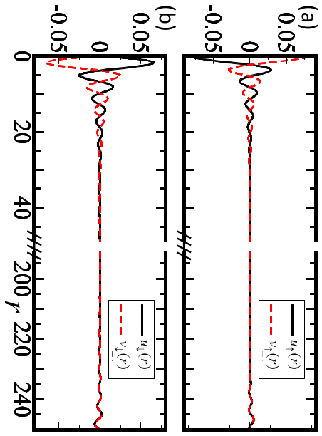
In Fig. 3, we plot the quasiparticle energy at different angular momentum channels. We see only at the channel, there is a unique Majorana zero energy solution. At non-zero channels, there are two discrete energy levels: one is the edge state, the other is the vortex core state. This can be clearly seen from the corresponding eigenwavefunctions for these two energy levels at the channel, which are plotted in Fig. 4. The continuous spectrum in Fig. 3 corresponds to the bulk excitations. Inside the vortex core, the first excited state above the zero energy mode is at the channel and the corresponding energy difference is called the minigap. The minigap is the energy gap that protect the Majorana zero energy state from finite temperature and disorder effects, therefore its magnitude is crucially important for the observation of non-Abelian statistics of quasiparticles in this system.
The non-Abelian topological property of the Majorana zero energy states at the channel originates from their special forms of the wavefunctions , , which lead to a self-Hermitian Bogoliubov quasiparticle operator, . Specifically, the quasiparticle wavefunctions around the vortex core satisfy , as clearly seen from Fig. 5. Chosen an artificial overall phase for the wavefunction (10), it is easy to show the Bogoliubov quasiparticle operator defined in Eq. (9) satisfies . Note that cannot be the electron creation or annihilation operator because it does not obey the anticommutation relation for electrons. Instead , the quasiparticle defined by is called a Majorana fermion. The exchange statistics of two Majorana quasiparticle excitations in two vortex cores are not the simple Fermi statistics: they can be either Abelian or non-Abelian in the degenerate subspace spanned by the Majorana operators in a set of vortices [1].


Interestingly, the wavefunctions still oscillate spatially even deep inside the bulk region. Such an oscillation makes it difficult to realize a single qubit gate for universal TQC using the tunneling between two vortices [45]. We also observe the zero energy edge states around the boundary, which satisfy , in contrast to in the vortex core. The wavefunctions and vanish at the boundary, as expected. An analytic explanation for the observed relation of the chiral edge modes is provided in Appendix C. We emphasize that zero energy state in the vortex core and the edge must appear simultaneously because Majorana zero energy modes only come in pairs (either between two vortices or between a vortex and the edge).

In Figs. (6,7,8), we plot three different quasiparticle energies with respect to various physical parameters: (i) the ground state energy in the vortex core at the channel. In certain parameter region, this state is the zero energy Majorana mode; (ii) the ground state energy in the vortex core at the channel. In the parameter region with the zero energy modes, this energy corresponds to the minigap ; (iii) the first excited energy at the channel. As we can see from Fig. 3, it corresponds to the minimum bulk excitation energy. Fig. 6 shows the dependence of these quasiparticle energies on the Zeeman field . We see the Majorana zero energy state exists only in the region . In this region, the minigap first increases rapidly to a level , and then decreases slowly with increasing . With a very large , all electrons occupy the spin down states, and there is no superconducting pairing. Therefore the decrease of the minigap with increasing is expected. Note that is larger than the typical minigap for a regular (s-wave or chiral p-wave) superconductor/superfluid [43]. To characterize the dependence of the minigap on the uniform bulk pairing gap , we numerically calculate for different and plot it in Fig. 9. We see in the region , is roughly proportional to . When , the minigap decreases because is now very close to . In general, may be a linear combination of and .

In Fig. 7, we see the zero energy modes disappear in the region . As expected, the minigap has a maximum at . only changes slightly when the chemical potential varies. In Fig. 8, we plot the quasiparticle energy with respect to the spin-orbit coupling strength . We see the minigap has a strong dependence on . initially increases quickly with a growing , and reaches the maximum, then decreases very slowly for large . This is expectable because the Rashba spin-orbit coupling provides the necessary chirality for the zero energy states. When , the coupling between spin up and down states vanishes, and a pure -wave superconductor does not have the zero energy modes.

The zero energy modes in the vortex core can be probed by bringing a STM tip close to the vortex core in experiments. The resulting tunneling conductance can be written as[44]
| (11) |
where is the voltage bias, represents different energy level, is the tunneling current, is the operation temperature of the STM, is the Fermi-Dirac distribution, and the derivative of is with respect to . In Fig. 10, we plot the STM tunneling conductances at different radius of the vortex core, which show clear zero energy peaks coming from the zero energy states. The other peaks correspond to other vortex core states at the angular momentum channels. The first peaks around the zero energy are at the channels. The distance between the peak centers at , channels is a measurement of the minigap. There is also an asymmetry of the peak strengths at . Because of the symmetry , in the BdG equation, we only need the terms in Eq. (11). Therefore the magnitudes of the peaks at positive or negative are proportional to and respectively. Generally, , leading to the asymmetric peaks around . In particular, we find the peak for at the negative disappears, which means must be zero for the minigap state (i.e., , state). As we can see from Eq. (15), in the minigap state involves the basis states and which are zero at because the Bessel function .

IV Effects of impurities
In a realistic TQC platform, both Majorana zero energy states and minigaps need be robust in the presence of impurities. A general argument on the robustness of zero energy states is based on the particle-hole symmetry in the BdG equation, which ensures its energy spectrum to be symmetric upon , that is, the and states must come in pairs. However, the zero energy does not come in pairs in a BdG equation (see Fig. 3). Therefore a local small perturbation cannot destroy this symmetry and shifts the zero energy to a finite energy that must emerge simultaneously with another state with an energy . Currently, the robustness of the magnitude of the minigap in the presence of impurities is still not clear. In the following, we consider three types of rotationally invariant impurities and study their effects on the zero energy states and the minigaps in the vortex core. Interestingly, we find that impurities may actually increase the minigaps in the vortex.


First, we consider a spin-independent Gaussian impurity
| (12) |
in the BdG equation (8) for a vortex, where is the impurity strength, is the half-width of the impurity potential that is comparable to the size of the vortex core. In Fig. 11, we plot the quasiparticle energies with respect to in the presence of a Gaussian impurity (12). In a regular s-wave superconductor, it is expected that such an impurity potential can couple different quasiparticle excitation states, and thus modify the energy spectrum. This can be seen in Fig. 11 in the parameter region without the zero energy states. We find that the zero energy states in the region are very robust even for a large impurity potential . More interestingly, we find that, by comparing with Fig. 6, the presence of the Gaussian impurity potential can increase the magnitude of the minigaps significantly. In Fig. 12, we plot the minigap and the bulk excitation gap in the presence of a Gaussian impurity potential. We see the minigap approaches the bulk excitation gap for a large . This enhancement of the minigap can be understood by considering the fact that the impurity potential can repulse (or attract) electrons and enlarge the energy level splitting between different discrete states in the vortex core. In practice, we may add a Gaussian type of potential at the vortex center to increase the minigaps and ensure the corresponding topological protection from finite temperature effects.

Secondly, we consider a magnetic impurity potential , whose effects on the zero energy modes and minigaps are shown in Fig. 13. Such an impurity potential acts as a spatially localized Zeeman field. No matter the local Zeeman field is along the same (Fig. 13a) or opposite (Fig. 13b) direction as the original Zeeman field , the zero energy states do not change and the minigaps are enhanced significantly. Note that in both cases the impurity does have a significant impact on the quasiparticle energies in the region .
Finally, we consider random impurity potentials
| (13) |
and , where are random frequencies (see the inset in Fig. 14a for the spatial profile of the random potential). This potential still has significant amplitudes outside the vortex core region. In Fig. 14, we find that the critical for the existence of the zero energy modes is smaller than the expected . It may originate from the long range property of the random potential, whose average around the vortex core shifts the chemical potential . Therefore the critical point is shifted to . For a magnetic random impurity , the corresponding critical point shifts to . However, the minigaps are small in these parameter regions, therefore they cannot be used as a TQC platform even the zero energy states exist. Only in the region , the zero energy states and the minigaps are robust against impurities.
So far the impurity potentials have been chosen to be rotationally invariant to simplify the numerical calculation. Non-rotationally invariant potentials couple different angular momentum channels and thus are difficult to simulate numerically. In a realistic situation, vortices in superconductors are often pinned by impurities so that the centers of the impurities and vortices are the same to minimize the free energy of the system. Such overlapping of the centers provides one justification of our choice of rotationally invariant impurity potentials. More generally, an impurity potential may be expanded as
| (14) |
where is the rotationally invariant part, while the corresponds to the non-rotationally invariant part. For instance, a Gaussian impurity potential located at instead of can be written as , where is the modified Bessel functions. Because the eigenstates of the BdG equation (8) have fixed angular momentum , only couples states with the same , while couples states with different . We can treat the impurity potential as a perturbation to the original BdG Hamiltonian. The first order energy correction to the zero energy state is because around the vortex. The second order correction because of the coexistence of and in the energy spectrum. Therefore the zero energy states are preserved by the particle hole symmetry in the BdG equation, as discussed at the beginning of this section. As to the minigap state, we see the first order correction only depends on the rotationally invariant part. The non-rotationally invariant part only yields a second or higher order correction to the minigap, which is generally small and may be neglected.
V Conclusion
In conclusion, we show that Majorana zero energy states and minigaps of quasiparticle excitations in a vortex are robust in a heterostructure composed of an s-wave superconductor, a spin-orbit-coupled semiconductor thin film, and a magnetic insulator. By numerically solving BdG equations with a vortex in a cylinder geometry, the dependence of Majorana zero energy states and minigaps on various physics parameters of the system (Zeeman field, chemical potential, spin-orbit coupling strength) is characterized. In certain parameter region, the minigap is proportional to the pairing gap , instead of for a regular chiral -wave superconductor/superfluid. The existence of the zero energy chiral edge state at the boundary is demonstrated both analytically and numerically. The STM tunneling conductance in the vortex core shows pronounced peaks at the zero energy as well as the minigap energy, which can be used to measure the zero energy state and the minigap. We show that the Majorana zero energy states are robust in the presence of various types of impurities. Surprisingly, we find that impurity potentials may greatly enhance the magnitudes of the minigaps. Therefore they can be induced intentionally in the heterostructure to enhance the topological protection of the non-Abelian platform. We believe our characterization of the behaviors of the zero energy modes and the minigaps in different parameter regions will help the design of a realistic semiconductor-superconductor heterostructure system for the experimental observation of non-Abelian statistics and the physical implementation of TQC in the future.
Acknowledgement: We thank Sumanta Tewari for helpful discussion. This work is supported by the DARPA-YFA (N66001-10-1-4025), DARPA-MTO (FA9550-10-1-0497), and the ARO (W911NF-09-1-0248).
Appendix A Numerical method for solving the BdG equation
Appendix B Finite size effect
In an infinite large system, the zero energy modes always exist in the parameter region [30]. In Ref. [30], the existence of the zero energy modes was proven by solving the BdG equation separately in and out the vortex core edge and matching the boundary condition at the vortex edge. A step function for the pairing gap has been used in this case to simplify the calculation. The zero energy modes exist when the number of unknown coefficients of the wavefunctions is equal to the number of independent constraints (vortex edge boundary conditions and normalization of the wavefunction), which occurs in the parameter region . However, there will be additional constraints in the system boundary, therefore zero energy solutions do not exist generally in a finite size system, that is, the quantum well state may destroy the zero energy modes when the size of the material or the confining potential is small enough.

To describe the finite size effect, we consider the parameter region , where the spin-orbit coupling and proximity induced superconductivity are not important. In this region, the BdG matrix (15) is diagonal, and the zero energy solution exists when
| (21) |
Here we take . We see there are zero energy modes only at some special . When exceeds , the lowest two eigenvalues are and , and the lowest energy branch reaches its local maximum at
| (22) |
where the integer is determined by
| (23) |
is the -th zero of the Bessel function and satisfies , therefore the maximum energy is
| (24) |
As an example, we consider the parameter , , and use the pairing gap from the s-wave superconductor. In Fig. (15), we plot the lowest two quasiparticle energies with respect to for two different sizes of the system . We see when is big enough, the fitting function () is a good approximation to the oscillation amplitude of the ground state. While at a small , the amplitude is much smaller than . It is clear when is big, the oscillation amplitude is strongly suppressed. In practice, we choose the parameters , , and the finite size effects can barely be seen and thus be neglected, as clearly demonstrated in Fig. (6).
Appendix C Chiral edge states at the channel
At the channel, the BdG equation for the zero energy state can be written as
| (25) |
where
| (26) |
. The BdG equation can be further reduced to a matrix differential equation
| (27) |
where the parameter and for nondegenerate zero energy states. These conditions yield and . It has been shown in Ref. [30] that only in the parameter region , , there is an unique zero energy solution. Here we show that a zero energy chiral edge state exists in the parameter region , .
As we can see from Fig. 2, the pairing gap decreases from its bulk value to zero at the boundary. For simplicity, we approximate the radial dependence around the boundary with a step function: for , and for , where is the coherence length of around the edge. Because is very large, the BdG equation (27) reduces to
| (28) |
around the boundary. In the region , the solution of Eq. (28) is given by with the constraint
| (29) |
The characteristic equation for is . There are four solutions of Eq. (28) which are well behaved at the edge: (), where , , , , are four solutions of Eq. (29). The full wavefunction in the region can be written as .
Far from the boundary, where , we can expand the solution as a series in
| (30) |
where are the corresponding spinors. The zeroth order coefficient satisfies the following equation:
| (31) |
The higher order coefficients can be calculated from using a set of recursion relations. The characteristic equation has 4 complex root for , same as that in Ref. [30]. Because Im is required for a physical solution, there are three independent roots only in the parameter region , , which yields three independent coefficients. Together with the four independent coefficients , , , , in the region , and seven constraints (match of and at , the boundary condition , and the normalization of the wavefunction), we can obtain a unique zero energy edge state at the boundary. However, the chiral edge state wavefunction satisfies instead of for the vortex core state, as clearly seen from Fig. 5.
References
- [1] C. Nayak, S. H. Simon, A. Stern, M. Freedman, S. Das Sarma, Rev. Mod. Phys. 80, 1083 (2008).
- [2] S. Das Sarma, M. Freedman, C. Nayak, Phys. Today
- [3] G. Moore, and N. Read, Nucl. Phys. B 360, 362 (1991).
- [4] C. Nayak, and F. Wilczek, Nucl. Phys. B 479, 529 (1996).
- [5] N. Read and D. Green, Phys. Rev. B 61, 10267 (2000).
- [6] S. Das Sarma, M. Freedman, and C. Nayak, Phys. Rev. Lett. 94, 166802 (2005).
- [7] A. Stern and B. I. Halperin, Phys. Rev. Lett. 96, 016802 (2006).
- [8] P. Bonderson, A. Kitaev, and K. Shtengel Phys. Rev. Lett. 96, 016803 (2006).
- [9] B. Rosenow, B. I. Halperin, S. H. Simon, and Ady Stern Phys. Rev. Lett. 100, 226803 (2008).
- [10] D. A. Ivanov, Phys. Rev. Lett. 86, 268 (2001).
- [11] A. Stern, F. von Oppen, E. Mariani, Phys. Rev. B 70, 205338 (2004).
- [12] S. Das Sarma, C. Nayak, and S. Tewari, Phys. Rev. B 73, 220502 (R) (2006).
- [13] S. Tewari, S. Das Sarma, D. H. Lee, Phys. Rev. Lett. 99, 037001 (2007).
- [14] S.Tewari, S. Das Sarma, C. Nayak, C. Zhang, and P. Zoller, Phys. Rev. Lett. 98, 010506 (2007).
- [15] S. Tewari, C. Zhang, S. Das Sarma, C. Nayak, D.-H. Lee, Phys. Rev. Lett. 100, 027001 (2008).
- [16] C.-H Cheng, and S.-K Yip, Phys. Rev. Lett., 95, 070404 (2005).
- [17] V. Gurarie, L. Radzihovsky, and A. V. Andreev, Phys. Rev. Lett. 94, 230403 (2005),
- [18] V. Gurarie and L. Radzihovsky, Phys. Rev. B 75, 212509 (2007).
- [19] S. S. Botelho and C. A. R. Sa de Melo, J. Low Temp. Phys. 140, 409 (2005).
- [20] C. Zhang, S. Tewari, and S. Das Sarma, Phys. Rev. Lett. 99, 220502 (2007).
- [21] A. Y. Kitaev, Ann. Phys. (N.Y.) 321, 2 (2006).
- [22] L.-M. Duan, E. Demler, M. D. Lukin, Phys. Rev. Lett. 91, 090402 (2003).
- [23] C. Zhang, V.W. Scarola, S. Tewari, S. Das Sarma Proc. Natl. Acad. Sci. USA 104, 18415 (2007).
- [24] C. Zhang, S. Tewari, R. M. Lutchyn, S. Das Sarma, Phys. Rev. Lett. 101, 160401 (2008).
- [25] M. Sato, Y. Takahashi, S. Fujimoto, Phys. Rev. Lett. 103, 020401 (2009).
- [26] L. Fu and C. L. Kane, Phys. Rev. Lett. 100, 096407 (2008).
- [27] L. Fu and C. L. Kane, Phys. Rev. Lett. 102, 216403 (2009).
- [28] A. R.Akhmerov, J. Nilsson, C. W. J. Beenakker, Phys. Rev. Lett. 102, 216404 (2009).
- [29] L. Fu, Phys. Rev. Lett. 104, 056402 (2010).
- [30] J. D. Sau, R. M. Lutchyn, S. Tewari, S. Das Sarma, Phys. Rev. Lett. 104, 040502 (2010).
- [31] T. D. Stanescu, J. D. Sau, R. M. Lutchyn, and S. Das Sarma, Phys. Rev. B 81, 241310(R) (2010).
- [32] P. A. Lee, arXiv:0907.2681.
- [33] X.-L. Qi, T. L. Hughes, and S.-C. Zhang, arXiv:1003.5448.
- [34] S. Tewari, J. D. Sau and S. Das Sarma, Ann. Phys. 325, 219, (2010).
- [35] J. Alicea, Phys. Rev. B 81, 125318 (2010).
- [36] J. D. Sau, S. Tewari, R. Lutchyn, T. Stanescu, and S. Das Sarma, arXiv:1006.2829.
- [37] J. D. Sau, S. Tewari, S. Das Sarma, arXiv:1004.4702.
- [38] R. M. Lutchyn, J. D. Sau, S. Das Sarma, Phys. Rev. Lett. 105, 077001 (2010).
- [39] J. D. Sau, R. M. Lutchyn, S. Tewari, S. Das Sarma, Phys. Rev. B 82, 094522 (2010).
- [40] J. Linder, and A. Sudbø, Phys. Rev. B 82, 085314 (2010)
- [41] Yu. A. Bychkov and E.I. Rashba, JETP Lett. 39, 78, (1984).
- [42] A. R. Akhmerov, Phys. Rev. B 82, 020509 (2010).
- [43] N. B. Kopnin and M. M. Salomaa, Phys. Rev. B 44, 9667 (1991).
- [44] F. Gygi and M. Schlüter, Phys. Rev. B 43, 7609 (1991).
- [45] M. Cheng, R. M. Lutchyn, V. Galitski, and S. Das Sarma, Phys. Rev. Lett. 103, 107001 (2009).