Can the Big Bang Singularity be avoided by a single scalar field?

Taotao Qiu Note: qiutt@mail.ihep.ac.cn Affiliation: Physics Department, Chung-Yuan Christian University, Chung-li, Taiwan 320

Abstract

In this note, we investigate the possibility of avoiding the Big Bang singularity with a single scalar field which couples non-minimally to gravity. We show that in the case that gravity couples linearly to the field, some severe conditions on the field’s potential have to be imposed. However, in non-linear case, it is quite generic to avoid the singularity with single scalar field.

I introduction

The Big Bang Singularity (BBS) is a notorious problem that present in Standard Big Bang Theory as well as inflation theory [1]. People have made a lot of efforts in solving this problem, and lots of mechanisms have been carried out, among which there are scenarios from string theory, quantum gravity theory and so on. Either reduced from these theories, or directly arisen from the effective field theory, we are able to obtain a bounce solution in 4-dimensional space-time. Bouncing cosmologies, especially non-singular ones, has gained more and more development in many aspects [2]. As an alternative of the standard theory in the early universe, it can not only avoid BBS, but also gives well favored observational effects compared to the astronomical data, such as scale invariant power spectrum and suppression of CMB low quardrupole on large scales [3]. Besides, a scenario of bouncing cosmology can give rise to large nongaussianities [4].

If we take our universe to be flat, thus within the framework of Einstein’s General Relativity in 4 dimensional space-time, a bounce is usually realized by Quintom matter [5]¹¹ 1 Of course there are many other alternatives which lead to a bounce, such as non-scalar fields or non-perfect fluids [6]. We thank the anonymous referee to remind us this.. As has been briefly proved in [5], in order for a bounce to happen, where the scale factor of the universe contracted to some value and then expanded, the Hubble parameter has to evolve from a negative value to a positive one. It will cause the equation of state of the universe will be less than $-1$ , violating the Null Energy Condition (NEC). Generally, some Phantom part will get involved that makes the physics unclear [7].

However, this dilemma can be ameliorated in many ways, such as to introduce non-scalar fields, or higher derivative operators and so on. One of the simplest ways is to go with the help of non-minimal coupling to Gravity [8]. In quantum gravity in curved space-time, it is argued that the existence of the non-minimal coupling term is required by the quantum corrections and renormalization [9]. This coupling includes scalar-tensor theories where the Ricci scalar couples to the field through the term $F(\phi)R$ [10] (as will be called “linear coupling” for convenience), which contains Brans-Dicke theory [11] or dilaton theory [12, 13], see [14] for a comprehensive review. Since the inclusion of non-minimal coupling term can drive cosmic acceleration with a wider class of potential than usually considered, it can also be utilized as inflaton in the early time [15] and dark energy at current epoch [16]. With the help of the non-minimal coupling, a single scalar field can also behave like systems of multi-degree-of-freedom without really involving a ghost field, such as having its equation of state (EoS) cross the cosmological constant boundary as a “Quintom” matter [17]²² 2 For Quintom investigations please see [18] and the following literature, one can also see [19] for a review.. Moreover, a great deal of non-minimal coupling theories can find their equivalence to the modified gravity theories [20].

In this paper we study the possibility of realizing bouncing scenario with a single scalar field non-minimally coupled to Gravity. We find that generally speaking, it does work as expected, except that for some specific case where Gravity couples linearly, some constraints have to be imposed on the field action. The paper is organized as follows: in section II we shortly demonstrate the general case for a non-minimal coupling field to drive a bounce, in section III and IV we investigate the linear coupling case and non-linear coupling case respectively, while conclusions come in the last section.

II general conditions for a single field to avoid Big Bang Singularity

To begin with, let us consider the most general action containing one scalar field and gravity, of which the two components are coupled in a very general form:

S=\int d^{4}x\sqrt{-g}\{\frac{f(R,\phi)}{2\kappa^{2}}+P(X,\phi)\}~,

(1)

where $\kappa^{2}\equiv 8\pi G$ and the metric used here is $g_{\mu\nu}=diag[1,-a^{2}(t),-a^{2}(t),-a^{2}(t)]$ . $X$ denotes the kinetic term of the field: $X\equiv\frac{1}{2}\nabla_{\mu}\phi\nabla^{\mu}\phi$ . What we’re working throughout this note is under Jordan frame³³ 3 As is well-known, the non-minimal coupling can be got rid of by performing the conformal transformation and redefining the scalar field. In that case, a bounce may not occur. This is due to the physical difference between Jordan and Einstein frames, in which the evolutions of the universe are not the same. We want to clarify this in some future work.. By variation of the action we can easily obtain the Friedmann Equations:

	$\displaystyle-\frac{f(R,\phi)}{2}-\kappa^{2}P(X,\phi)+\kappa^{2}P_{X}\dot{\phi^{2}}+3(\dot{H}+H^{2})f_{R}-3H\dot{f_{R}}$	$\displaystyle=$	$\displaystyle 0~,$		(2)
	$\displaystyle\frac{f(R,\phi)}{2}+\kappa^{2}P(X,\phi)-f_{R}(\dot{H}+3H^{2})+\ddot{f_{R}}+2H\dot{f_{R}}$	$\displaystyle=$	$\displaystyle 0~,$		(3)

where $f_{R}\equiv\frac{df}{dR}$ , and the equation of motion for the field $\phi$ is:

-P_{X}\Box\phi-P_{XX}\nabla_{\mu}X\nabla^{\mu}\phi-P_{X\phi}\nabla_{\mu}\phi\nabla^{\mu}\phi+P_{\phi}+\frac{f_{\phi}}{2\kappa^{2}}=0~.

(4)

where $\Box\phi=\ddot{\phi}+3H\dot{\phi}$ and similarly $f_{\phi}\equiv\frac{df}{d\phi}$ is the derivative of $f(R,\phi)$ with respect to the field $\phi$ .

As mentioned before, for a flat universe with standard Einstein Gravity in 4-dimensional space-time, a bounce happens only when the Null Energy Condition (NEC) is violated. We can learn from Einstein Equations that this leads to the vanishing of Hubble parameter $H$ with a positive time derivative, namely $H=0$ and $\dot{H}>0$ at the bounce point [5]. Substituting the first condition to the above equations one gets:

	$\displaystyle 3\ddot{f}_{R}+\kappa^{2}(\rho+3P)+f=0~,$		(5)
	$\displaystyle\dot{H}=\frac{f+2\kappa^{2}\rho}{6f_{R}}>0~.$		(6)

In following sections, we will analyze in detail the application of these conditions to the non-minimal coupling scalar field. Before starting, we would like to classify the coupling term into two categories according to its properties: one is a more specific case that the Gravity couples linearly to the field, and the other is a more general case which refers to non-linear coupling. Actually, these two categories are very different due to the different numbers of degree of freedom in the background equations. Due to this reason, it may cause very different conclusions.

III Category I: Gravity coupling linearly to the field

III.1 general solution

Among the various possible forms the coupling terms may have, it is the simplest to study the one that Ricci scalar couples linearly to the field, which is easy to get a renormalizable theory without any suppression. Moreover, as differ from its non-linear counterpart, in this case the higher order derivative of $R$ is zero, thus higher order time derivatives of $H$ will not get involved into the background equations. To study the general solution of this case, let us assume that $f(R,\phi)=R(1-F(\phi))$ , where the first term in the bracket denotes the standard term from General Relativity, and the second comes from the non-minimal coupling. From Eqs. (2) and (3), one can get:

	$\displaystyle-\frac{R(1-F(\phi))}{2}+\kappa^{2}\rho+3\dot{H}(1-F(\phi))$	$\displaystyle=$	$\displaystyle 0~,$		(7)
	$\displaystyle\frac{R(1-F(\phi))}{2}+\kappa^{2}P(X,\phi)-\dot{H}(1-F(\phi))\ddot{-F(\phi)}$	$\displaystyle=$	$\displaystyle 0~,$		(8)

which can be furtherly simplified to a very neat form:

	$\displaystyle-3H^{2}(1-F)+\kappa^{2}\rho+3H\dot{F}$	$\displaystyle=$	$\displaystyle 0~,$		(9)
	$\displaystyle 2\kappa^{2}XP_{X}+2\dot{H}(1-F(\phi))-2XF_{\phi\phi}-F_{\phi}\ddot{\phi}$	$\displaystyle=$	$\displaystyle 0~.$		(10)

In deriving these equations, we have made use of the fact $\rho=2XP_{X}-P$ and $\dot{X}=\dot{\phi}\ddot{\phi}$ . The last one of the above equations gives

\ddot{\phi}=\frac{2\kappa^{2}XP_{X}+2\dot{H}(1-F(\phi))-2XF_{\phi\phi}}{F_{\phi}}~.

(11)

For $H=0$ , we have

	$\displaystyle\rho$	$\displaystyle=$	$\displaystyle 0~,$		(12)
	$\displaystyle\dot{H}$	$\displaystyle=$	$\displaystyle-\kappa^{2}\frac{\rho_{X}(2\kappa^{2}XP_{X}-2XF_{\phi\phi})+\rho_{\phi}F_{\phi}}{3F_{\phi}^{2}+2\kappa^{2}\rho_{X}(1-F)}~.$		(13)

In deriving the last equation we also made use of Eq. (4). We can see from above that for case of gravity coupling linearly to scalar field, a bounce requires the rhs of the above equation to be larger than 0 as well as the energy density equals to 0. This can be viewed as a general condition for this case.

III.2 single scalar field with canonical form

At first let us consider the simplest case in which the field has a standard canonical form:

P(X,\phi)=\frac{1}{2}\partial_{\mu}\phi\partial^{\mu}\phi-V(\phi)~,

(14)

where $V(\phi)$ is its potential. Thus the energy density of the field $\rho=\frac{1}{2}\dot{\phi}^{2}+V(\phi)$ . The condition of $\rho=0$ requires that at the bounce point $\frac{1}{2}\dot{\phi}^{2}+V(\phi)=0$ , or equivalently $V(\phi)=-\frac{1}{2}\dot{\phi}^{2}$ . It can be straightforwardly seen that as long as $\dot{\phi}\neq 0$ at this point, one needs $V(\phi)<0$ , namely, a potential containing negative values at least at some region is required, while a positive-definite potential as usual doesn’t work. But is that the case even for the possible case where $\dot{\phi}=V(\phi)=0$ , though it refers to a very specific point in $(\phi,\dot{\phi})$ space and needs strong fine-tuning? To see this, let’s take a look at the other condition of $\dot{H}>0$ , which then indicates:

\frac{V_{\phi}F_{\phi}}{3F_{\phi}^{2}+2\kappa^{2}(1-F)}<0~.

(15)

where we used $\rho_{\phi}=V_{\phi}$ as well as $\rho_{X}=1$ . From this equation we notice that $V_{\phi}$ can be either larger or less than 0, depending on the form of $F(\phi)$ . For example, if we assume that $F(\phi)=\kappa^{2}\xi\phi^{2}$ , then the condition is $\xi\phi V_{\phi}<0$ . But anyway, as long as $V_{\phi}\neq 0$ at the bouncing point where $V(\phi)=0$ , there will inevitably be some region where $V(\phi)<0$ . So this will be a generic constraint on the potential of the field. In usual case, this will break down the positive-definition of the energy density, which causes unphysics. However, here it is fine both because of the positive kinetic term and the effects of gravity. Thus, after some proper choice of parameters, we can still get a self-consistent system.

As a further study, we also derived the second derivative of $H$ with respect to $t$ at the bouncing point. It appears to be:

$\displaystyle\ddot{H}$	$\displaystyle=$	$\displaystyle\frac{1}{[2\kappa^{2}(1-F)+3F_{\phi}^{2}]^{2}}\{[2\kappa^{2}(1-F)+3F_{\phi}^{2}][\kappa^{2}(-2\kappa^{2}\dot{\phi}\ddot{\phi}-4\dot{H}\dot{\phi}F_{\phi}-4H\ddot{\phi}F_{\phi}-4H\dot{\phi}^{2}F_{\phi\phi}$	(16)
		$\displaystyle-V_{\phi\phi}F_{\phi}\dot{\phi}-V_{\phi}F_{\phi\phi}\dot{\phi}+F_{\phi\phi\phi}\dot{\phi}^{3}+2F_{\phi\phi}\dot{\phi}\ddot{\phi})-12H\dot{H}F_{\phi}^{2}-12H^{2}F_{\phi}F_{\phi\phi}\dot{\phi}]$
		$\displaystyle+(2\kappa^{2}F_{\phi}\dot{\phi}-6F_{\phi}F_{\phi\phi}\dot{\phi})[\kappa^{2}(-\kappa^{2}\dot{\phi}^{2}-4H\dot{\phi}F_{\phi}-V_{\phi}F_{\phi}+F_{\phi\phi}\dot{\phi}^{2})-6H^{2}F_{\phi}^{2}]\}~.$

It can be straightforwardly read off that for the $\dot{\phi}=V(\phi)=0$ case (note that $H=0$ ), $\ddot{H}$ will vanish at the bouncing point. This means that in this case, the velocity of Hubble parameter always reaches its extreme value when passing through the bouncing pivot. This is a new property that hasn’t been pointed out by other authors in the literature.

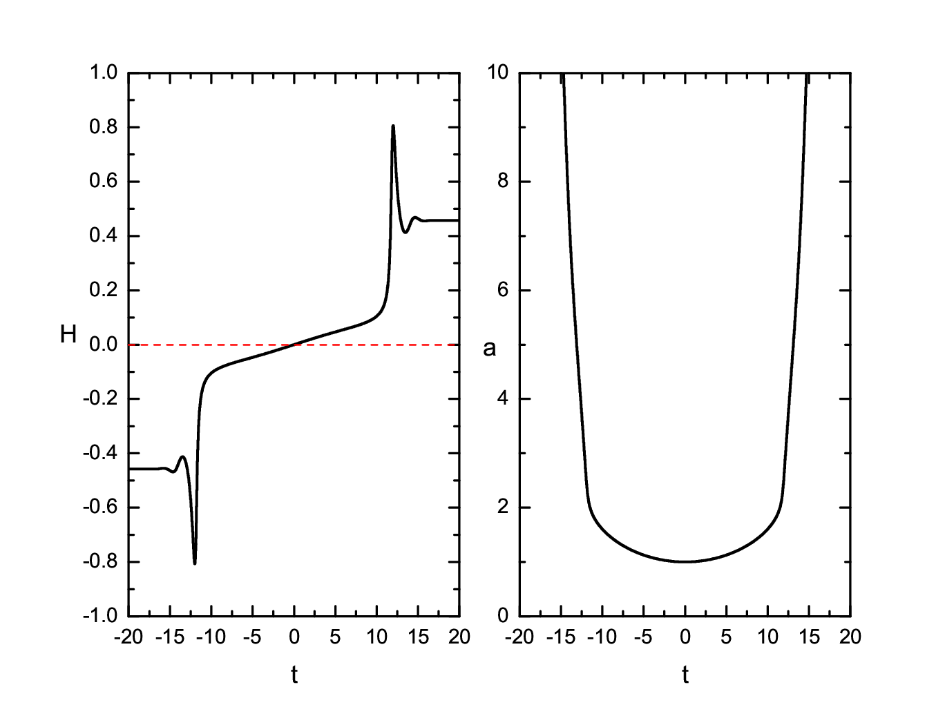
In order to support our analytical calculation, we also try to find some regions in parameter space which can give good numerical results. In order to satisfy the constraints on the potential, we take into account two forms of potentials: 1) $V(\phi)=\frac{1}{2}m^{2}\phi^{2}-V_{0}$ and 2) $V(\phi)=V_{0}(e^{\lambda\phi^{2}}-\frac{1}{2})$ . We add some negative zero-point energy to the potential to let it get some negative region. For the coupling term, we choose $F(\phi)=\kappa^{2}\xi\phi^{2}$ , where $\xi$ is some coupling constant. In Figs. 1 and 2 we show some numerical calculations on Hubble parameter $H$ and scale factor $a$ . We can see that a bounce can happen naturally with $H$ crosses the zero divide line. This indicates that by this way, the Big Bang Singularity can be avoided.

Refer to caption — Figure 1: The case of canonical single scalar field and linear non-minimal coupling. The potential is chosen to be $V(\phi)=\frac{1}{2}m^{2}\phi^{2}-V_{0}$ and the coupling term is $RF(\phi)=\kappa^{2}\xi R\phi^{2}$ . The parameter is chosen to be $m=0.1m_{pl}$ , $V_{0}=0.005m_{pl}^{4}$ and $\xi=-1.0$ , and the initial conditions are $\phi_{i}=0.473m_{pl}$ , $\dot{\phi}_{i}=0.061m_{pl}^{2}$ .

III.3 single scalar field with DBI form

Beside canonical ones, there is another form of scalar field that is very common used in cosmology: the Dirac-Born-Infeld (DBI) form. Actions of this form effectively describes tachyon dynamics, which can be obtained naturally in string theory [21]. Moreover, it can also drive the acceleration of the universe and can act as inflaton [22] and dark energy [23]. As inflationary models inspired by the string theory, the DBI action non-minimally coupled to gravity has also been investigated in the literature, cf. Ref. [24]. Here we study the last case to see whether it can avoid the Big-Bang Singularity.

The DBI lagrangian containing non-minimal coupling term is:

P(X,\phi)=-V(\phi)\sqrt{1-2\alpha X}~,

(17)

where $\alpha$ is some positive constant. Its energy density can be calculated as $\rho=2XP_{X}-P=\frac{V(\phi)}{\sqrt{1-2\alpha X}}$ . One can also obtain its equation of state and sound speed square by their definitions:

w\equiv\frac{P}{\rho}=2\alpha X-1~,~~~~~c_{s}^{2}\equiv\frac{P_{X}}{\rho_{X}}=\sqrt{1-2\alpha X}~,

(18)

which shows that this kind of action is stable under classical perturbations $(0<c_{s}^{2}<1)$ with Quintessence-like behavior ( $-1<w<0$ ).

From (17) we obtain the equation of motion for the scalar field:

-\frac{\alpha V}{(1-2\alpha X)^{\frac{1}{2}}}\Box\phi-\frac{\alpha^{2}V}{(1-2\alpha X)^{\frac{3}{2}}}\dot{X}\dot{\phi}-\frac{\alpha V_{\phi}}{(1-2\alpha X)^{\frac{1}{2}}}\dot{\phi^{2}}-V_{\phi}\sqrt{1-2\alpha X}-\frac{RF_{\phi}}{2\kappa^{2}}=0~,

(19)

where we get:

\ddot{\phi}=-\frac{[2\kappa^{2}(3H\alpha V\dot{\phi}+V_{\phi})+RF_{\phi}(1-2\alpha X)^{\frac{1}{2}}](1-2\alpha X)}{2\kappa^{2}\alpha V}

(20)

and the Friedmann equation:

	$\displaystyle 3H^{2}(1-F(\phi))=\kappa^{2}\frac{V(\phi)}{\sqrt{1-2\alpha X}}+3HF_{\phi}\dot{\phi}~,$		(21)
	$\displaystyle\dot{H}=\frac{-\kappa^{2}[\kappa^{2}\frac{2\alpha^{2}V^{2}X}{(1-2\alpha X)^{\frac{1}{2}}}+\alpha VHF_{\phi}\dot{\phi}+F_{\phi}(1-2\alpha X)(3H\dot{\phi}\alpha V+V_{\phi})-2F_{\phi\phi}X\alpha V]-6H^{2}F_{\phi}^{2}(1-2\alpha X)^{\frac{3}{2}}}{2\kappa^{2}(1-F)\alpha V+3F_{\phi}^{2}(1-2\alpha X)^{\frac{3}{2}}}~.$		(22)

From above we can see that the first condition at the bounce point $\rho=0$ only requires $V=0$ , which is looser than that of the canonical scalar field case. Moreover, $F_{\phi}V_{\phi}<0$ is still required by the second condition $\dot{H}>0$ . Therefore, in order to have a bounce, a region of negative value of $V(\phi)$ is also inevitable.

We also make the numerical calculations, with the potential of the form $V(\phi)=V_{0}(e^{\lambda\phi^{2}}-\frac{1}{2})$ and some proper parameter choice. The bounce happens naturally from the view of the plots. As a side remark, one may notice that due to different initial conditions, the model may present various behaviors. From Fig. (3) we can see that, the hubble parameter varies very fast after the bounce, from increasing to decreasing, indicating that the universe will enter into a moderate accelerating or decelerating expansion phase soon. While from Fig. (4), one may note that the hubble parameter experienced a period of slow variation. This indicates that it is also possible to give rise to an inflationary period after bounce, although we will not discuss in detail as it goes beyond current topic.

IV Category II: Gravity couples non-linearly to the field

As a comparison, in this section, we will focus on a more general case where, in the coupling term, Gravity possesses a non-linear form. The most general form of basic equations comes from Eq. (2-4), However, for the sake of simplicity, we only discuss about the canonical field (14). Therefore, we can derive the Friedmann equations and the equation of motion explicitly:

	$\displaystyle\ddot{H}$	$\displaystyle=$	$\displaystyle\frac{1}{18Hf_{RR}}[(Rf_{R}-f)/2-3Hf_{R\phi}\dot{\phi}+\kappa^{2}(\frac{{\dot{\phi}}^{2}}{2}+V(\phi))-3f_{R}H^{2}]-4H\dot{H}~,$		(23)
	$\displaystyle\dddot{H}$	$\displaystyle=$	$\displaystyle\frac{1}{6f_{RR}}[H(f_{RR}\dot{R}+f_{R\phi}\dot{\phi})-2f_{R}\dot{H}-\kappa^{2}\phi^{2}-f_{RRR}{\dot{R}}^{2}-2f_{RR\phi}\dot{\phi}\dot{R}-f_{R\phi\phi}{\dot{\phi}}^{2}-f_{R\phi}\ddot{\phi}]-4H\ddot{H}-4{\dot{H}}^{2}~,$		(24)

where

\ddot{\phi}+3H\dot{\phi}+V_{\phi}-\frac{f_{\phi}}{2\kappa^{2}}=0~.

(25)

Since the non-linear term of Gravity has been involved, the higher order derivatives of $H$ appears in the equation, which makes the equations difficult to solve analytically. But as the order of derivative increases, the number of effective degrees of freedom becomes more, and it will be easier to violate NEC and realize the bouncing process.

Figs. 5 and 6 show that a canonical field with coupling term contains logarithm function of $R$ . The logarithm coupling may seem strange, however, one can find the similar form in previous phenomenological studies, see e.g. [25]. We can see from the plot that with proper choice of parameter, this kind of coupling may also give rise to a bounce scenario. Fig. 7 is the plot of universe behavior for the coupling of $R^{2}$ to some exponential potential of $\phi$ . This kind of potential looks like the dilaton potential in string theory [12]. With this kind of coupling, the universe can also pass through the bouncing point smoothly.

V conclusions and discussions

In this note we investigated the possibilities of a single scalar field giving rise to a bouncing scenario in the very early universe, with some non-minimal coupling to gravity. Along with some explicit examples, we showed that it is quite possible. However, for the common case that Gravity couples linearly to the field, the field will suffer from some severe conditions, such as abandoning the positive-definition of the potential. For other cases where Gravity couples non-linearly, it will be more free to get a bounce since more degrees of freedom have been evoked.

The realization of bounce with non-minimal coupling field is important in the sense that, with the involvement of Gravity, one no longer needs any ghost field to violate NEC, which might cause problems. Recently there have been many works on construction of bouncing cosmologies within the framework of non-minimal coupling theories, which have some relation to our work while focus more on their fundamental origins [26]. Furthermore, it is expected that with proper choice of the coupling form, it is also possible to obtain right amount of observational signatures to meet the data, and to give rise to some new features and predictions for future experiments, for example, a recent work shows that the matter bounce scenario with non-minimal coupling will give rise to scale-invariant spectrum and large particle productions [27]. All these fancy topics are left for the forthcoming work.

Acknowledgments

The author thanks Kazuharu Bamba, Prof. Je-An Gu, Prof. Anupam Mazumdar, Prof. Yunsong Piao and Yi Wang for useful suggestions at the beginning of the work. The research is supported in parts by the National Science Council of R.O.C. under Grant No. NSC96-2112-M-033-004-MY3 and No. NSC97-2811-033-003 and by the National Center for Theoretical Science.

References

[1] S. W. Hawking, and G. F. R. Ellis, The large scale structure of space-time, Cambridge University Press (1973); A. Borde and A. Vilenkin, Phys. Rev. Lett. 72, 3305 (1994).
[2] M. Novello and S. E. P. Bergliaffa, Phys. Rept. 463, 127 (2008).
[3] Y. S. Piao, B. Feng and X. m. Zhang, Phys. Rev. D 69, 103520 (2004); Y. S. Piao, Phys. Rev. D 71, 087301 (2005); see also Y. F. Cai, T. t. Qiu, J. Q. Xia and X. Zhang, Phys. Rev. D 79, 021303 (2009); Y. F. Cai, T. t. Qiu, R. Brandenberger and X. m. Zhang, Phys. Rev. D 80, 023511 (2009).
[4] Y. F. Cai and X. Zhang, JCAP 0906, 003 (2009); Y. F. Cai, W. Xue, R. Brandenberger and X. Zhang, JCAP 0905, 011 (2009).
[5] Y. F. Cai, T. Qiu, Y. S. Piao, M. Li and X. Zhang, JHEP 0710, 071 (2007).
[6] S. D. Brechet, M. P. Hobson and A. N. Lasenby, Class. Quant. Grav. 25, 245016 (2008).
[7] S. M. Carroll, M. Hoffman and M. Trodden, Phys. Rev. D 68, 023509 (2003); J. M. Cline, S. Jeon and G. D. Moore, Phys. Rev. D 70, 043543 (2004).
[8] J. P. Abreu, P. Crawford and J. P. Mimoso, Class. Quant. Grav. 11, 1919 (1994); S. S. Bayin, F. I. Cooperstock and V. Faraoni, Astrophys. J. 428, 439 (1994); R. Fakir, arXiv:gr-qc/9810054; J. w. Lee, S. Koh, C. Park, S. J. Sin and C. H. Lee, Phys. Rev. D 61, 027301 (2000); T. Biswas, A. Mazumdar and W. Siegel, JCAP 0603, 009 (2006); T. Biswas and A. Mazumdar, Phys. Rev. D 80, 023519 (2009); T. Biswas, T. Koivisto and A. Mazumdar, arXiv:1005.0590 [hep-th]; Y. F. Cai and E. N. Saridakis, arXiv:1007.3204 [astro-ph.CO]; For review see A. Mazumdar and J. Rocher, arXiv:1001.0993 [hep-ph].
[9] N. A. Chernikov and E. A. Tagirov, Annales Poincare Phys. Theor. A 9 (1968) 109; C. G. . Callan, S. R. Coleman and R. Jackiw, Annals Phys. 59 (1970) 42; N. D. Birrell and P. C. W. Davies, Quantum Fields In Curved Space, Cambridge University Press (1982).
[10] Y. Fujii and K. Maeda, The Scalar-Tensor Theory of Gravitation,” Cambridge University Press (2003); B. Boisseau, G. Esposito-Farese, D. Polarski and A. A. Starobinsky, Phys. Rev. Lett. 85, 2236 (2000).
[11] C. Brans and R. H. Dicke, Phys. Rev. 124, 925 (1961).
[12] M. Gasperini and G. Veneziano, Astropart. Phys. 1, 317 (1993); M. Gasperini and G. Veneziano, Phys. Rept. 373, 1 (2003).
[13] K. Bamba and M. Yoshimura, Prog. Theor. Phys. 115, 269 (2006).
[14] T. P. Sotiriou and V. Faraoni, Rev. Mod. Phys. 82, 451 (2010); A. De Felice and S. Tsujikawa, Living Rev. Rel. 13, 3 (2010); A. De Felice and S. Tsujikawa, arXiv:1005.0868 [astro-ph.CO].
[15] L. F. Abbott, Nucl. Phys. B 185, 233 (1981); T. Futamase and K. i. Maeda, Phys. Rev. D 39, 399 (1989); T. Futamase, T. Rothman and R. Matzner, Phys. Rev. D 39, 405 (1989); R. Fakir and W. G. Unruh, Phys. Rev. D 41, 1783 (1990); L. Amendola, D. Bellisai and F. Occhionero, Phys. Rev. D 47, 4267 (1993); V. Faraoni, Phys. Rev. D 53, 6813 (1996).
[16] J. P. Uzan, Phys. Rev. D 59, 123510 (1999); T. Chiba, Phys. Rev. D 60, 083508 (1999); L. Amendola, Phys. Rev. D 60, 043501 (1999); L. Amendola, Phys. Rev. D 62, 043511 (2000); V. Faraoni, Phys. Rev. D 62, 023504 (2000); V. Faraoni, Class. Quant. Grav. 22, 3235 (2005); S. Nojiri and S. D. Odintsov, eConf C0602061, 06 (2006) [Int. J. Geom. Meth. Mod. Phys. 4, 115 (2007)]; M. Szydlowski, O. Hrycyna and A. Kurek, Phys. Rev. D 77, 027302 (2008). For non-minimal coupling of Gauss-Bonnet type see e.g. K. Bamba, Z. K. Guo and N. Ohta, Prog. Theor. Phys. 118, 879 (2007); S. Nojiri, S. D. Odintsov and M. Sasaki, Phys. Rev. D 71, 123509 (2005) and the following literature.
[17] R. G. Cai, H. S. Zhang and A. Wang, Commun. Theor. Phys. 44, 948 (2005); L. Perivolaropoulos, JCAP 0510, 001 (2005); P. S. Apostolopoulos and N. Tetradis, Phys. Rev. D 74, 064021 (2006); R. Gannouji, D. Polarski, A. Ranquet and A. A. Starobinsky, JCAP 0609, 016 (2006); B. M. Leith and I. P. Neupane, JCAP 0705, 019 (2007); K. Nozari and M. Pourghasemi, JCAP 0810, 044 (2008); A. K. Sanyal, Gen. Rel. Grav. 41, 1511 (2009); E. Elizalde, S. Nojiri and S. D. Odintsov, Phys. Rev. D 70, 043539 (2004); L. Amendola and S. Tsujikawa, Phys. Lett. B 660, 125 (2008).
[18] B. Feng, X. L. Wang and X. M. Zhang, Phys. Lett. B 607, 35 (2005). For quintom with higher derivatives see M. z. Li, B. Feng and X. m. Zhang, JCAP 0512, 002 (2005); X. F. Zhang and T. Qiu, Phys. Lett. B 642, 187 (2006), for quintom with non-scalar fields see Y. F. Cai and J. Wang, Class. Quant. Grav. 25, 165014 (2008).
[19] Y. F. Cai, E. N. Saridakis, M. R. Setare and J. Q. Xia, arXiv:0909.2776 [hep-th]; T. Qiu, Mod. Phys. Lett. A 25, 909 (2010).
[20] E. E. Flanagan, Phys. Rev. Lett. 92, 071101 (2004); T. Chiba, Phys. Lett. B 575, 1 (2003); E. E. Flanagan, Class. Quant. Grav. 21, 417 (2003); G. J. Olmo, Phys. Rev. D 72, 083505 (2005); T. P. Sotiriou, Class. Quant. Grav. 23, 5117 (2006); V. Faraoni, Phys. Rev. D 75, 067302 (2007); M. Capone and M. L. Ruggiero, Class. Quant. Grav. 27, 125006 (2010).
[21] R. G. Leigh, Mod. Phys. Lett. A 4, 2767 (1989); O. Aharony, S. S. Gubser, J. M. Maldacena, H. Ooguri and Y. Oz, Phys. Rept. 323, 183 (2000); R. C. Myers, JHEP 9912, 022 (1999), see also A. Sen, JHEP 9808, 012 (1998); A. A. Gerasimov and S. L. Shatashvili, JHEP 0010, 034 (2000) and references therein.
[22] G. R. Dvali and S. H. H. Tye, Phys. Lett. B 450, 72 (1999); S. Kachru, R. Kallosh, A. D. Linde, J. M. Maldacena, L. P. McAllister and S. P. Trivedi, JCAP 0310, 013 (2003); E. Silverstein and D. Tong, Phys. Rev. D 70, 103505 (2004); see also D. A. Easson and R. Gregory, Phys. Rev. D 80, 083518 (2009); D. A. Easson, S. Mukohyama and B. A. Powell, Phys. Rev. D 81, 023512 (2010).
[23] G. W. Gibbons, Phys. Lett. B 537, 1 (2002); S. Mukohyama, Phys. Rev. D 66, 024009 (2002); D. Choudhury, D. Ghoshal, D. P. Jatkar and S. Panda, Phys. Lett. B 544, 231 (2002); T. Padmanabhan, Phys. Rev. D 66, 021301 (2002); J. g. Hao and X. z. Li, Phys. Rev. D 66, 087301 (2002); J. S. Bagla, H. K. Jassal and T. Padmanabhan, Phys. Rev. D 67, 063504 (2003); E. J. Copeland, M. R. Garousi, M. Sami and S. Tsujikawa, Phys. Rev. D 71, 043003 (2005); E. N. Saridakis and J. Ward, Phys. Rev. D 80, 083003 (2009). For Quintom models whose EoS can cross $-1$ see Y. f. Cai, M. z. Li, J. X. Lu, Y. S. Piao, T. t. Qiu and X. m. Zhang, Phys. Lett. B 651, 1 (2007); S. G. Shi, Y. S. Piao and C. F. Qiao, JCAP 0904, 027 (2009).
[24] D. A. Easson and R. Gregory, Phys. Rev. D 80, 083518 (2009); D. A. Easson, S. Mukohyama and B. A. Powell, Phys. Rev. D 81, 023512 (2010).
[25] B. Feng, H. Li, M. z. Li and X. m. Zhang, Phys. Lett. B 620, 27 (2005).
[26] M. R. Setare, J. Sadeghi and A. Banijamali, Phys. Lett. B 669, 9 (2008); K. Nozari, M. R. Setare, T. Azizi and S. Akhshabi, arXiv:0901.0090 [hep-th]; K. Nozari and S. D. Sadatian, arXiv:0904.4029 [gr-qc].
[27] T. Qiu and K. C. Yang, arXiv:1007.2571 [astro-ph.CO].