August 24, 2026
WKB analysis of edge states in graphene in a strong magnetic field.
Abstract
We investigate the fine structure of the edge states energy spectrum for zigzag and armchair ribbons of graphene in a strong magnetic field. At low energy, the spectra can be described by an effective Schrödinger Hamiltonian with a double well potential, symmetric in the zigzag case and asymmetric in the armchair case. We develop a semiclassical formalism based on the WKB approximation to calculate analytically the energy spectrum for the two types of edges, including regions which were not studied earlier. Our results are in very good quantitative agreement with numerical calculations. This approach leads to a qualitative description of the spectra in terms of the quantization of unusual classical orbits in the real space.
pacs
03.65.Sq, 73.22.Pr, 73.43.CdI Introduction
The fascinating properties of graphene originate from its perfect two-dimensional character and from its unusual electronic structure where valence and conduction bands touch at two inequivalent points of reciprocal space. In the vicinity of these two points, the dispersion relation is linear and charge carriers behave as massless Dirac fermions[1] with striking consequences on the electronic properties, like the unusual 2D quantum Hall effect.[2, 3] Recent studies have also addressed electronic properties of confined graphene structures like dots, rings or nanoribbons. In particular, nanoribbons have been suggested as potential candidates for replacing electronic components in future nanoelectronic and nanospintronic devices.[4, 5] In that perspective, the role of edge states is essential. In the absence of magnetic field, edge states can emerge for particular types of edges.[6, 7] Such localized electronic states can be described analytically at low energy by using the Dirac equation with the appropriate boundary conditions.[8] More recent theoretical works have investigated the metallic nature of such edge states by considering staggered on-site potentials,[9] surface perturbations,[10] spin-orbit coupling,[11] edge dopping,[12] and sophisticated terminations of the honeycomb lattice.[13, 14, 15] Experimental efforts have been performed to observe different natures of edges[16, 17, 18] and study charge transport in ribbons.[19, 20]
This paper deals with the structure of edge states in a strong magnetic field, a problem which has been the subject of recent interest. Although this problem is somehow reminiscent of the case of usual 2D electrons,[21, 22] it is much richer since here charge carriers are massless particules and the structure of the edge states depends of the nature of the edges. In particular, Brey and Fertig first calculated within the tight-binding model the band structures of ribbons in a magnetic field with two types of boundary conditions: the so-called zigzag and armchair edges.[26] In addition, they have shown that these two types of edges can be described at low energy by a Schrödinger Hamiltonian with a harmonic potential. In the zigzag case, this potential is similar to the one of the usual integer quantum Hall problem,[21] whereas in the armchair case, the potential presents a specific asymmetry. Moreover, these edge states have been recently investigated numerically in graphene rings,[23] and in graphene ribbons by considering an anisotropic hopping parameter,[24] or by taking account for a possible quantum Hall ferromagnetism.[25]
However, the energy dependence of the Landau levels when approching the edges has only been discussed briefly. The goal of this paper is to investigate in details the fine structure of the edge states energy spectrum for zigzag and armchair ribbons and provide a complete quantitative analytical description within the WKB approximation. The paper is organized as follows: In section II, we recall and discuss in details the tight-binding spectra for zigzag and armchair ribbons with and without magnetic field. When a field is applied, we point out peculiar features of the edge states which we describe analytically in the rest of the paper. Following the procedure suggested by Brey and Fertig,[26] we derive in section III a simple effective Hamiltonian (essentially the squared Dirac Hamiltonian) with a potential depending on the boundary conditions. Then, in section IV, we present a semiclassical framework to calculate analytically the low energy spectra. Two methods are used: the first one is based on the Bohr-Sommerfeld quantization of the action and leads to a simple qualitative picture in terms of classical skipping orbits in section V. However, this method does not properly describe the case where the classical cyclotron radius is of the order of the distance to the edge. Therefore, we develop a more sophisticated semiclassical approach, based on the WKB approximation, that leads to analytical quantitative results in agreement with numerical calculations. The details of this approach are given in the appendix. We conclude in section VII.
II Tight-binding spectrum
II.1 Zero magnetic field
We briefly recall the band structure of infinite graphene ribbons within the tight-binding picture. For that purpose, we first consider the Hamiltonian of an infinite 2D sheet of graphene, and we use the Bloch theorem in both and directions. As the honeycomb lattice has two carbon atoms per cell (that we call A and B, see Fig. 1), the Bloch wave function is written as :
| (1) |
where are the vectors of the triangular Bravais lattice. Then, within the tight-binding model, the Hamiltonian is written as :
| (2) |
in the basis of the two sublattices where is the hopping parameter between nearest neighbors and with :
| (3) |
where and are the basis vectors of the triangular Bravais lattice with . The lattice parameter is related to the carbon-carbon distance nm by . The dispersion relation given by (see Fig. 2(a)) consists in two bands which touch at the corners of the first Brillouin zone (FBZ). The positions of these points are given by the condition , that is :
where and are the basis vectors of the reciprocal lattice. The spectrum is linear near these points. The choices of the unit cell and of the axes are illustrated in Fig. 1(a). The positions of the so-called and Dirac points are shown in Fig. 1(b), where we have also indicated their projections onto the axis and .

We consider now infinite ribbons with either zigzag or armchair edges. In these finite geometries, the Bloch theorem can be used only along the infinite direction, and the boundary condition along the finite direction yields a finite number of bands. These bands, computed in the tight-binding model, are displayed in Figs. 2 (d-e). It is seen that the spectra of these ribbons correspond to the projection of the 2D spectrum along the axis (armchair edge) or the axis (zigzag edge). The projected points and coincide in the armchair case but they do not in the zigzag case. This remark illustrates the fact that for the armchair case, the two valleys are admixed by the boundary condition as we will discuss later. Finally, note that the flat level between the two points and for zigzag edge is not captured by the projection of the bulk result. This zero energy state is localized near the edges and its existence depends on the boundary conditions.[7, 8, 28] This edge state exists whitout any magnetic field, contrary to the edge states in the quantum Hall regime which are studied in this paper.

From now on, we define the geometry of the armchair and zigzag ribbons as shown in Fig. 3 : the ribbon is infinite along the direction and it has a finite width in the direction. Within this convention, we have for the zigzag ribbons and for the armchair ones.

II.2 Perpendicular magnetic field
We now apply a perpendicular magnetic field on each type of ribbon and calculate numerically the band structure within the tight-binding model.[26] The finite width of the ribbons along the axis leads us to work with the Landau gauge . Because of the vector potential , the hopping parameter (taken as unity in the rest of the paper), takes a Aharonov-Bohm phase , where is the magnetic flux quantum. We now study the low energy spectrum for a given magnetic flux through an elementary plaquette. In Fig. 4, we show the low energy tight-binding spectra for the zigzag ribbon with and without magnetic field in the same plot. The spectra for the armchair case are shown in Fig. 5. The zero field cones are progressively transformed into flat Landau levels with the expected behaviour.[29]


We now comment on several important features of these spectra which to our knowledge have not been discussed in the literature. Since in the chosen Landau gauge, a state is centered at the position along the direction, where is the magnetic length, the variation of the energy levels can be interpreted as a function of this position, as redrawn in Figs. 6 and 7. In these figures, we have indicated the position of the edges along the direction, at low energy. Indeed, the position of one edge is fixed by the position of the Dirac points in zero field and the other edge is located at a distance where is the width of the ribbon and where . As the two valleys are not admixed in the zigzag case, this operation must be performed for both and valleys, as seen in Fig. 6. Therefore, it is clear that the dispersive character of the levels corresponds to the edge states, as first discussed by Halperin in the context of the integer quantum Hall effect of massive particules in two dimensional gases.[21] However, the band structure for graphene is more complex and depends on the type of edge as we discuss now. For the zigzag edge, we first emphasize that, inside a given valley, the spectrum is not symmetric: the energy levels are not identical on left and right sides. Moreover, exactly at the left and right edges, the energy levels take peculiar values : they alternatively take the value of higher bulk Landau levels . This correspondence is displayed by horizontal color lines in Fig. 6. More precisely, for the valley, we have the relation with (blue lines) on the left edge whereas we have (green lines) with for the right edge. In addition, we have the same structure in the valley, provided the role of the two edges is permuted. This remarkable distribution of the edge states will be explained in section IV.3.

The armchair case, in Fig. 7, is quite different. Each Landau level is doubly degenerate, a direct consequence of the valley admixing. The degeneracy lifting takes place close to the edge with a non monotonous behaviour for one every two levels, that will be explained in section IV.3.

In the following we present a qualitative and quantitative description of these spectra within a semiclassical analytical approach.
III Low energy effective Hamiltonian
III.1 The bulk Hamiltonian
At low energy, the Hamiltonian (2) can be linearized around the two Dirac points and . Expanding as in each valley, the tight-binding Hamiltonian is then replaced by a linearized Dirac-like Hamiltonian :
| (4) |
which describes the two uncoupled valleys in the basis , where and is the lattice spacing. The eigenfunctions can be expressed as the superposition of the contributions of the two valleys, so that we can write :
In the magnetic field , and within the Landau gauge , we perform the Peierls substitution . Then we introduce the dimensionless variables , and . Since , the Hamiltonian in a magnetic field reads :
| (10) | |||
Next, it is useful to work with the squared Hamiltonian which is diagonal. We introduce the dimensionless effective Hamiltonian as :
| (16) |
which defines four effective Schrödinger equations :
| (17) |
with
where the potentials and are given by :
| (23) | |||||
| (24) |
and are displayed in Fig 8. Thus, the effective Hamiltonian simply describes only two different harmonic oscillators. Because of the non-commutativity of the operators and , the two harmonic potentials and are shifted by one energy level. From (17) and (III.1), one obtains two different Schrödinger equations, one with the potential for and , and the other one with the potential for and .
The eigenvalues of the original Hamiltonian (III.1) are obtained from the dimensionless eigenvalues of the effective Hamiltonian as :
| (25) |
In the Landau gauge we have used, the wave function is a plane wave along the direction and now reads :

The eigenvalues are the Landau levels associated with the eigenfunctions of the harmonic oscillator as follows :
This is illustrated in Fig. 8. The effect of the edges is to modify the potentials (23) and (24) and consequently the components of the wave functions and the energy spectrum. These modifications depend on the nature of the edge which yields to specific boundary conditions. In the two following subsections, we derive the effective Schrödinger equations for zigzag and armchair edges.
III.2 Zigzag edges
To treat the zigzag edges of a graphene ribbon, we first recall that all the atoms on one edge belong to the same sublattice, and therefore, all the atoms on the opposite edge necessarily belong to the other sublattice. As the ribbon is periodic in the direction, we still write the low energy wave functions as in (III.1) but the components are not the eigenfunctions of the harmonic oscillator anymore. As the left edge is only made of A sites (see Fig. 3), the wave function on the B sites vanishes for i.e. . The situation is identical on the right edge at for the A sublattice : . As a consequence, we have the boundary conditions :
| (38) |
These boundary conditions do not admix the valleys which can still be described separately, as in the bulk system. Consequently, with the zigzag boundary conditions, we have four independent Schrödinger equations, one for each valley and for each sublattice, with four independent potentials , , and . Such boundary conditions can be accounted for by an infinite potential barrier either at or at , acccording to the sublattice and the valley. Namely, the potentials and are harmonic potentials that have to be cut in whereas the potentials and have to be cut in . Since the four edge problems are quite similar, we focus on the case of the right edge for the valley. Thus, the potential reads :
| (39) |
and is plotted in Fig. 9. Similarly, one can define , and .

As a matter of fact, the problem of a harmonic well with an infinite potential barrier (Fig. 9) is identical to the problem of a double symmetric harmonic well (Fig. 10), provided we only keep, in the latter, the eigenenergies associated with the eigenstates that vanish on the edge, that are the antisymmetric states. The interest of considering such a double symmetric well is that, as we will see in section III.3, both zigzag and armchair edges can be described by double harmonic wells, the difference being an energy shift between the two wells in the armchair case. We illustrate in Fig. 10 the double symmetric potential we finally consider in the effective Schrödinger equation for the right zigzag edge and the valley, that is :
| (40) | |||
| (41) |
The index refers to the antisymmetric solutions and we have performed the translations and , so that the right edge is now located in . The eigenenergies are calculated analytically within a WKB treatment introduced in section IV. The detailed calculations are explained in the appendix.

III.3 Armchair edges
We now consider the case of an armchair ribbon as displayed in Fig. 3(b). The corresponding low energy Hamiltonian is obtained from (4) by the substitution and . By keeping the same gauge as above, the Hamiltonian in the presence of a magnetic field now reads :
| (42) | |||
Of course, this new choice of axes does not affect the eigenvalues of the bulk problem and leaves the effective Hamiltonian defined in (16) unchanged, but the eigenfunctions have now the following form :
| (48) |
where the functions are the eigenfunctions of the harmonic oscillator. The phase factor originates from the orientation of the ribbon. Following the procedure suggested by Brey and Fertig,[26] we now construct an effective Hamiltonian which accounts properly for the armchair boundary conditions. Since, for this type of edge, we have the particular relation , as argued in section II, the wave functions now read :
where the components must satisfy specific boundary conditions. A crucial difference with zigzag ribbons is that armchair edges are constituted of both A and B sites. As a consequence, both components and must vanish on each side of the ribbon: and . From now on, we choose to explicit these boundary conditions for the left side at , what leads to :
| (57) |
Contrary to the zigzag case, the armchair boundary conditions admix the contributions of the two valleys for a given sublattice. In addition, since the Dirac Hamiltonian is first order, the continuity equations (57) on the wave function imply continuity of the derivatives. From (42) and (57) we obtain :
| (58) |
Next, as suggested by Brey and Fertig,[26] we build new functions as :
| (59) | |||||
where is the Heaviside function. Thus, the functions are solutions of a new effective Schrödinger equation with a potential which is for and for :
| (60) | |||
| (61) |
In order to take into account the armchair boundary conditions (57-58), we impose the functions to satisfy the continuity equations :
The asymmetric potential (61) is shown in Fig. 11. The asymmetry originates from the non-commutativity of with and corresponds to a shift in energy by one Landau level between the two uncoupled wells and . The asymmetric structure of is a consequence of the valley admixing imposed by the boundary conditions.

We now discuss the qualitative structure of the wave functions. The two combinations are built with four components . When the particule is far from the edge, the system is described by two independent potentials and so that the components take their bulk value given by (48). Now, close to the edge, the expressions of are modified. In particular, the boundary conditions (III.3) imply two types of solutions and , by matching the components in two different ways. We illustrate this point in Fig. 12 in the case where by showing a qualitative construction of the components . The eigenfunction has nodes whereas has nodes. As a consequence, the associated eigenvalues are lower than the eigenenergies , and the valley degeneracy of the energy spectrum is lifted, as seen in Fig. 5. This point is discussed quantitatively in section IV.3.
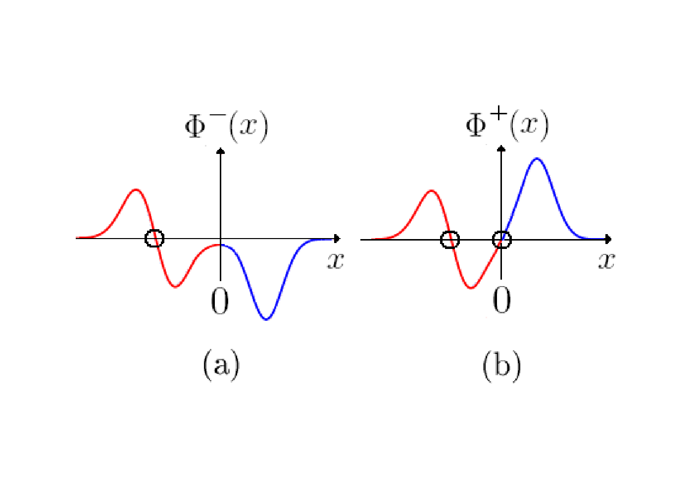
By imposing , the right edge can now be considered easily in the same way. We obtain a similar effective problem where the potential has been replaced by :
| (65) |
where we have performed the translations and for more commodity in the calculations in the next section. Thus, the potential that describes the right edge at is now centered in . The potential is displayed in Fig. 13.

IV Semiclassical treatment
The aim of this section is to calculate analytically the energy spectrum for both zigzag and armchair boundary conditions, by using a semiclassical formalism. The eigenenergies are solutions of effective Schrödinger equations in appropriate potentials: a double symmetric harmonic potential (Fig. 10) for the zigzag case and a double asymmetric harmonic potential (Fig. 13) for the armchair case. We develop here two approaches. In the first one (Sec. IV.1), we assume that the two wells of the potentials are uncoupled, and quantize the action with the Bohr-Sommerfeld rule. The second approach (Sec. IV.2), based on the WKB formalism, properly accounts for the overlap of the wave function between the two wells.
From now on, we only focus on the right edge of the ribbons, and take .
IV.1 Semiclassical quantization of the action
We first define the classical cyclotron radius . For the zigzag case, is given by as illustrated in Fig. 10. For the armchair case, since the potential is asymmetric, we need to define two classical cyclotron radii and (see Fig. 13). Next, we introduce an action associated with these potentials. Along a closed path, the action is given by :
| (66) |
where and are the positions of the turning points, and is either or . Such an action is quantized with the Bohr-Sommerfeld rule as :
| (67) |
where is an integer and is a function that encodes all the information on the connection procedure at the turning points. For a harmonic potential, . Here, for the double well potentials, is not a constant anymore, but depends on the energy and on the distance to the edge because of the overlap of the wave function between the two wells. We assume in this section that the two wells are uncoupled, so that we take as a constant.
Now we have to specify distinct regions in energy, each of them requiring an appropriate semiclassical treatment. These regions are delimited by horizontal thick lines in Figs. 10 and 13 and involve different expressions of the action given by (66).
IV.1.1 Zigzag ribbons
We consider the potential that describes the right zigzag edge for the valley (Fig. 10). We recall that the right edge is located at . For a given energy , we have to discuss two distinct regions : (region ) and (region ), where is the cyclotron radius.
- •
Region : . The turning points are defined by and so that the action (66) in the left well is simply :
(68) A simple calculation of the energies by quantizing with the constant value in (67) leads to the Landau levels with , and therefore to the spectrum in this region. The term originates from the energy shift of the potential . The rest of the spectrum near the right edge is given by the contribution of the other valley. Therefore, by treating the same way the potential , we find the spectrum with . Finally, we obtain a set of degenerated energies with , and a non degenerated level what gives the expected valley degenerated graphene energy levels for .
- •
Region : . The left turning point is unchanged but the right turning point is replaced by so that the action reads :
(69) where we have introduced the parameter . The spectrum depends now on the distance to the edge. The total action in the double well is quantized as . We recall that we have to keep only the antisymmetric solutions which have an odd number of nodes, what implies . Therefore, such a quantization leads to :
(70) We recover the result for a harmonic potential cut by an infinite barrier potential.[34] By identifying the two expressions (69) and (70), we finally obtain a set of self-consistent equations labeled by the integer for , from which we can extract the energy spectrum.
IV.1.2 Armchair ribbons
Because of the asymmetry of the potential , we have now to distinguish three regions (, , in Fig. 13). In each one, we consider two actions, for the left well and for the right well. In addition, the levels in the left or in the right well will be indexed by different integers . The energy is given by where (resp. ) is the cyclotron radius for the left (resp. right) well.
- •
Region : . In each well, the action still has the form given by (68), so that we write :
(71) By using the Bohr-Sommerfeld rule (67) with for both and , we find the energies into the left well and into the right well, and then . This leads to the degenerated Landau levels with and a non degenerated level .
- •
Region : . Now, because of the step in the potential, the action has the form given by (69), whereas is unchanged. The two actions read
(72) The action is still quantized as previously, what simply gives the spectrum with . As the wave function inside the right well does not totally vanish in , the situation is different than in the case of an infinite potential barrier. This suggests a choice closer to rather than for the quantization of the action . By doing so, we obtain an implicit equation in and from which we can extract the spectrum . Of course, we understand that the region is necessarly badly described by such an approach and specifically requires a more sophisticated method since cannot be a constant anymore.
- •
Region : . In this region, we need to consider the total action that reads :
(73) where the function is given in (69). This expression is still valid when crosses the edge. Since the two turning points both touch a harmonic potential, this action is simply quantized by the usual Bohr-Sommerfeld rule with what also leads to an implicit equation in and , where is a different integer than , since there are twice more solutions in this region than in the regions or .
The armchair spectrum obtained within this approach is shown in Fig. 17. It perfectly matches with numerical solutions of the Schrödinger equation (60) except around the intermediate region . In the following, we describe quantitatively all the regions by keeping and calculating the spectra of zigzag and armchair ribbons by accounting for the coupling between the two wells. We give now the general picture of the method which is detailed in the appendix.
IV.2 The WKB approach
In this section, we present a method based on the WKB formalism to account for the overlap of the wave function between the two wells. This approach is detailed in the appendix. Technically, it brings us to calculate the function . For this purpose, we express the wave function inside the left well within the WKB approximation as :
| (74) |
with a constant and where
| (75) |
is the partial action between the turning point and an arbitrary position inside the left well. Close to the right turning point , this approximation breaks down. In order to find a valid approximation of the wave function in this region, we linearise the harmonic potential so that the eigenfunctions of the Schrödinger equation are a combination of Airy functions, that is :
| (76) |
where and are constants and is a function that depends on the region , , , or , so that each region must be treated separately. By imposing the equality between and the asymptotic expansion of inside the well, we obtain a relation between the constants and the action which is given by the relation (66). We need to distinguish the cases and (Fig. 14), for which the matching condition gives :
| (77) |
where is a known function originating from the step between the energy at the turning point and the potential . The same procedure must be performed for the right well where we obtain similar relations between the ratio and the action calculated between the two turning points in the right well :
| (78) |
where is the left turning point in the right well.

To determine the ratio , we impose the continuity of the wave function and its derivative between the two wells. By doing so, we obtain one equation with the two unknown quantites and . Next, by injecting into (78), where the total action is calculated explicitly as a function of and , we obtain a second order polynomial in what yields two solutions. Because of the relation (77), the action is quantized as which is the Bohr-Sommerfeld quantization. Thus, the two solutions of the polynomial yield the two solutions .
Next, by using the formula (66), we calculate explicitly the expression of the action as a function of and , which we identify with the action given by the Bohr-Sommerfeld rule previously found. As we know the functions , we finally obtain two analytical self-consistent equations in and for a given , one with , the other one with . The spectrum can then be extracted for a given . The whole procedure must be performed for each region to where the action has different expressions as discussed in the previous section. All this study is detailed in the appendix for both the symmetric and the asymmetric potentials.
IV.3 Quantitative analytical results
We give here the spectra obtained for the effective potentials (zigzag case (41)) and (armchair case (65)), within the two semiclassical approaches introduced above.
IV.3.1 Symmetric potential (zigzag)
The energy levels of the double symmetric harmonic potential describing the contribution of the valley at the right zigzag edge (see Fig. 10) are shown in Fig. 15. The two regions and are separeted by a parabola of equation . In the spectrum of Fig. 15, we have only kept the higher energy solution of the double well problem, since they correspond to the eigenenergies of the antisymmetric eigenfunctions. The dashed lines correspond to the approximation where , what leads to an unphysical discontinuity around . The continuous lines represent the energy levels obtained within the WKB approximation. The solutions found with this method in regions and perfectly match at .

Next, we show in Fig. 16 the structure of the edge states spectrum in the valley for both the left and right edges. The right (blue) part of the spectrum, is the energy spectrum on the right edge calculated within the WKB method and already displayed in Fig. 16, whereas the left (red) part represents the edge states on the left side of the ribbon in the same valley. The effective problem for the left edge is obtained in a similar way than for the right edge (see section III.2) where we have considered the potential and the boundary condition . Note that we recover the particular relation with on the left edge and with for the right edge. This peculiar property of the edge states is due to the fact that we have to keep only the antisymmetric eigenfunctions of the double well problem. In particular, when , the double well is simply a single harmonic well, so as the bulk potenials. In addition, the shift of this distribution between the two edges is due to the shift in energy between the potentials and that respectively originate from the potentials and modified by the zigzag boundary conditions. We have emphasized this point by dashed lines in Fig. 16. This explains the remarkable structure of the zigzag edge states discussed in section II.2. Finally, the mirror symmetry between the valleys and emphasized in Fig. 6 is now clear, since the edge potentials into the valley, that are for the right edge and for the left edge, now originate from the bulk potentials and respectively with the zigzag boundary conditions.

IV.3.2 Asymmetric potential (armchair)
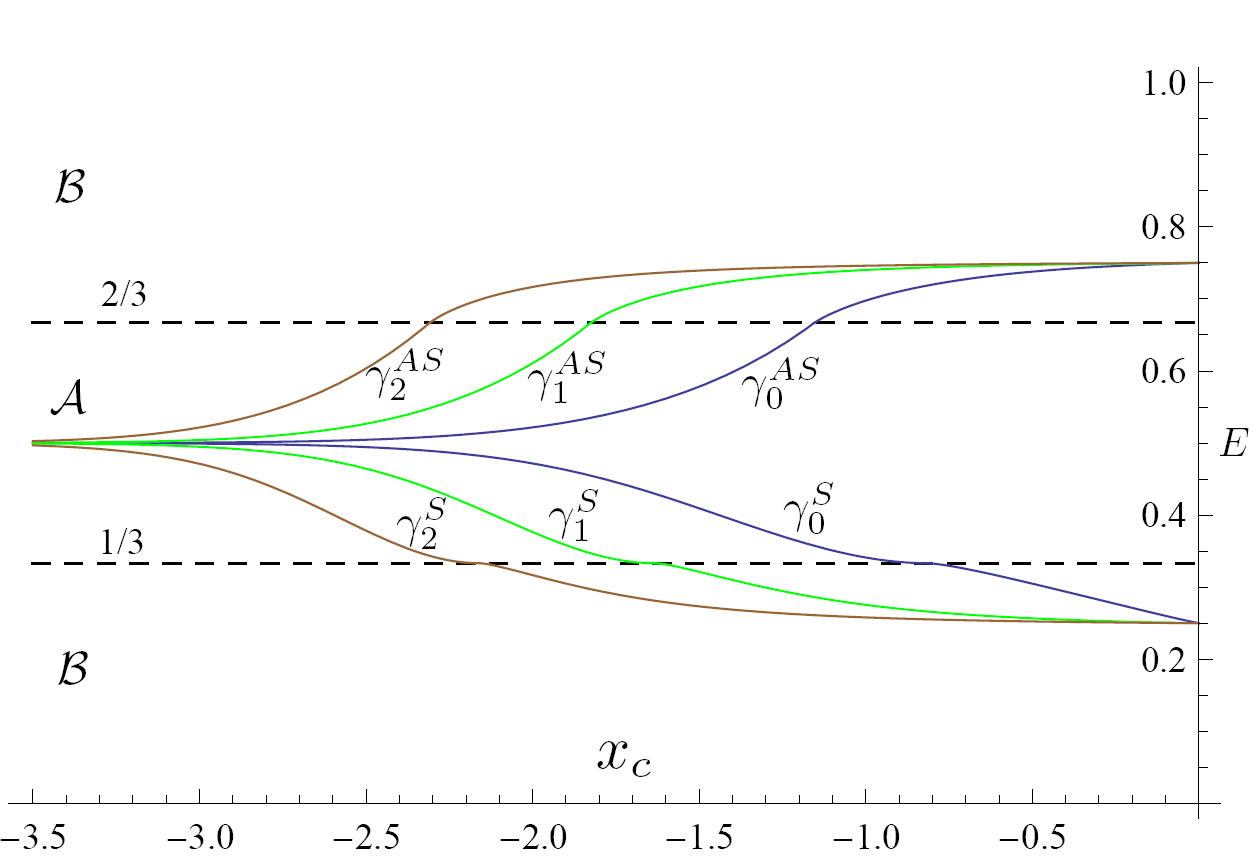
For the armchair case, we have to keep all the solutions of the double asymmetric potentials and . As discussed in section III.3 and illustrated in Fig. 12, the wave functions of the effective Schrödinger equation with armchair boundary conditions (60) have, for a given , either nodes or nodes, what leads to pairs of eigenenergies . The semiclassical energies are displayed in Fig. 17. The three regions , and are separeted by the parabola parametrized by and , that are and . Contrary to the simple semiclassical calculation with (discontinued brown lines), the WKB method gives a perfect matching between the three regions and is in very good agreement with numerical calculations (grey crosses).

V Quantized skipping orbits
In this section, we propose a simple interpretation of the results in terms of a semiclassical picture for skipping orbits. Consider the action associated with the effective Schrödinger equations with the potentials obtained for the zigzag case. These four equations (one per edge and per valley) describe the motion of a free massive particle in a magnetic field (all units being set to one) in the presence of an infinite potential barrier or the image of the harmonic potential, as illustrated in Figs. 9 and 10 for the right edge in the valley. From the classical equations of motion, the action along a closed trajectory for a given energy is simply related to the area enclosed by the corresponding periodic orbit :
| (79) |
so that the Bohr-Sommerfeld quantization rule (67) implies the quantization of the area
| (80) |
in our units where . In the bulk of the system, that is when the distance to the edge is larger than the cyclotron radius , we have simply
| (81) |
and the distances are measured in units of . This quantization implies the quantization of the cyclotron radius . Taking , , so that , we deduce the energy levels, , and obtain the bulk spectrum of Landau levels .
When becomes smaller than , the classical orbits skip along the wall represented by the infinite potential well, and they form open orbits. As already noticed[35], the area to be quantized is the area delimited by the skipping orbit and the wall. In this case, the action calculated in (69) has a very simple interpretation in terms of skipping orbits since the parameter has a clear geometrical meaning shown in Fig. 18. The action is nothing but the area enclosed by the skipping orbit :
| (82) |
We can now interpret semiclassically the energy spectra obtained in the above subsections.
For the zigzag edge, the two regions and in the spectrum (Fig. 15) can be associated to the two distinct cases represented in Fig. 18.
| (a) region , | (83) | ||||
| (b) region , |
from, which together with the relation , we have deduced the energy levels, except near the region .

For the armchair case, the situation is more involved, since we describe the classical motion of a massive particle in the presence of its shifted image (Fig. 19). Since the potential is asymmetric, we have defined two cyclotron radii related to the energy as . Now we have to consider three different cases corresponding to the regions , and in Fig. 17.
In the region where , the orbit and its image are both closed cyclotron orbits. The quantization of their area :
| (84) |
leads to the the energy levels given by , with , what quantize the cyclotron radii as and , the latest does not allow the level.
In the region where , the left orbit is still closed but its image is a skipping orbit. Keeping the notation , we have :
from which we obtain the energy levels in region . The degeneracy lift is classically explained by the fact that both orbits have a different structure. The left orbit is closed and its semiclassical energy is still , while the energy associated with the right skipping trajectory increases with . Note that it is in this peculiar region that an inversion of the slope occurs.
In the region where , both orbits are open and the area to be quantized is the total area
| (88) |
Since the action has almost doubled from region to region , the resulting energy spectrum is twice denser, and the two-fold degeneracy of the levels has been removed.

VI Two edges
Up to now, we have considered the evolution of the spectrum in the vicinity of one edge. If the two edges are sufficiently far apart compared to the cyclotron length , the spectrum can be treated independently on both sides. We now consider the case of a narrow ribbon, whose width is of the order of a few magnetic lengths. The low energy spectrum in a ribbon of width is shown on Fig. 20(a) and 21(b), respectively for zigzag and armchair ribbons.


In the zigzag case, in each valley, the spectrum clearly exhibits three different regions, which correspond to the geometry of the orbits depicted in Fig. 20(b) . Regions corresponds to bulk cyclotron orbits. Regions and have been already discussed and correspond to a skipping orbit along a single boundary (left or right). Each sublattice is characterized by a cyclotron orbit (in valley, small blue orbit for sites and large pink orbit for sites; the opposite for the valley). As explained in the text, in valley, the cyclotron orbits sees only the right edge and the cyclotron orbits sees only the left edge (the opposite in the valley). At high energy, the new region corresponds to the situation where both cyclotron orbits intersect the two boundaries. The black curves correspond to the situations where a cyclotron orbit precisely touches a boundary. Their equation is
| (89) |
where for the left edge and for the right edge. By a simple quantization of the areas shown in Fig. 20(b), one can obtain the full low energy spectrum in a very good approximation, excepted when the orbits graze the boundaries, that is in the vicinity of the black curves. It is obvious on this figure that the two edges do not play exactly the same role, and that, for a given valley, the spectrum is not exactly symmetric. Furthermore, in each valley, an additional dissymetry is seen at high energy because the linear approximation of the low energy Hamiltonian breaks (III.1) down.


The case of armchair boundary conditions is more involved. In Fig. 21(a), one can distinguish 9 regions, which corresponds to the geometries of the classical orbits depicted in Fig. 21(b). The black curves correspond to the situations where a cyclotron orbit precisely touches a boundary. Their equation is given by Eq. (89). Region corresponds to bulk cyclotron orbits. The blue cyclotron orbits are related to the and eigenfunctions, whereas the pink cyclotron orbits are related to the and eigenfunctions. Regions and have been already discussed and correspond to skipping orbits along a single boundary (left or right). In the intermediate regions and , only one of the two orbits touches the edge. At high energy, in the region , the two cyclotron orbits touch the two edges of the ribbon. The more exotic regions , and have a simple geometric interpretation in Fig. 21(b).
VII Conclusion
We have investigated the spectra of graphene ribbons in a magnetic field with zigzag and armchair boundary conditions. We have first revisited these spectra numerically and revealed a remarkable structure in the repartition of the edge states in zigzag ribbons, that we explain in this paper. We notice that these remarkable behaviours of the edge states could be observed by scanning tunneling microscopy (STM) or spectroscopy (STS) techniques.[30, 31, 32, 33]
Next we have described and calculated these edge states with simple analytic tools. For both types of ribbons, effective Schrödinger equations with a specific double well potential have been derived at low energy. This potential is asymmetric in energy when the valleys and are coupled (armchair edge) and symmetric otherwise (zigzag edge). The eigenenergies of these potentials have been calculated recently.[30] Another recent work[27] provided a semiclassical framework to study analytically the edge states for both zigzag and armchair edges, but, this approach does not furnish the full low energy spectrum. We have developped here two semiclassical methods to calculate the energy edge states analytically. A very simple one consists in using the Bohr-Sommerfeld quantization of the action related to the effective Schrödinger equations. This approximation captures the essential of the physical picture except when the cyclotron radius of the effective particule is of the order of the distance to the edge. This approach also reveals different regions as a function of the energy and the distance to the edge, where the skipping orbits are quantized in different ways. The second method is based on the WKB formalism, and accounts for the overlap of the wave function when it is close to the edge. Consequently, this more sophisticated analytical approach perfectly describes the edge states whatever the distance of the center of the cyclotron motion to the edge. In particular, it quantitatively describes an interesting region in the armchair case (called region in the paper) where the energy does not increase monotonously. This implies that the drift velocity along the edge may change in sign when the position varies. These WKB results perfectly fit numerical exact calculations.
Acknowledgments - We acknowledge useful discussions with J.-N Fuchs and M.-O. Goerbig. This work is supported by the NANOSIM-GRAPHENE project (ANR-09-NANO-016-01) of ANR/P3N2009.
*
Appendix A The WKB method
In the whole appendix, we define the classical action as half of the one defined in (66).
In this appendix, we present the detailed calculations on the energy levels within the WKB approximation, for the potential defined as :
| (90) |
The case has been introduced in section III.2 for the study of edge states in zigzag nanoribbons, while the case has been used in section III.3 to describe armchair ribbons.

A.1 Double symmetric harmonic well
We consider the peculiar case , that is a double symmetric harmonic potential :
| (91) |
For a given energy , we define the cyclotron radius as (Fig. 22). In addition, in the whole appendix, the factor in the definition of the action (66) is missing: the actions and are now defined as the half of those introduced in Sec. IV.
A.1.1 Region :
This case, characterized by , corresponds to the region in Fig. 22. We write the WKB wave functions in both wells and then the matching conditions in . As the potential is symmetric with , we focus on the left well (). The energy defines two classical turning points at positions and (Fig. 22). Within the WKB approximation, the connection procedure near implies that the wave function in the well reads :
| (92) |
where the left arrow indicates that this wave function matches the correct connection procedure near the left turning point . is a constant and is the partial action in the left well :
| (93) |
The above expression (92) breaks down near the second turning point . Near this point we linearize the potential as and the Schrödinger equation reads :
| (94) |
The solution of this equation is given by a combination of Airy functions :
| (95) | |||
| (96) | |||
| (97) |
where the right arrow indicates that this wave function must obey proper matching conditions near the right turning point . and are constants. Inside the well, this wave function has the asymptotic expansion :
| (98) |
| (99) |
The argument in the trigonometric functions can be related to the partial action between and
| (100) |
where is the total action in the left well. Therefore can be rewritten in the form :
| (101) |
with (idem for ). Then, we impose inside the well. This implies and what finally leads to the important relation :
| (102) |
As the two wells are identical, we obtain the same relation for the right well :
| (103) |
and, similarly to (95), the wave function in the right well reads near :
| (104) |
The next step is to impose the matching of the two wave functions and their derivatives in :
| (105) |
These matching conditions give the two equations :
from which the ratio is extracted as :
| (106) |
The symmetry of the potential implies , so that, from (102) and (103), we have . The relation (106) becomes a simple polynomial for the unknown quantity :
| (107) | |||||
whose solutions
| (108) |
correspond respectively to the symmetric and antisymmetric wave functions. The action is quantized by the condition , so that with , with two solutions for :
| (109) | |||||
| (110) |
In region , the action is very simply related to the energy, , so that from (110,110), we obtain the implicit equations :
| (111) | |||
| (112) |
where itself depends on the energy :
These implicit equations are solved numerically and we obtain the spectrum (region ) shown in Fig. 23.
A.1.2 Region :
This is the region illustrated in Fig. 22. The expression of the WKB wave function matching the correct connection procedure near is still given by Eq. (92). The second turning point in does not exist anymore, and we have to know the expression of the wave function near . It reads :
| (113) | |||||
| (114) | |||||
| (115) |
Far from , the Airy functions can be expanded to obtain :
where we have set :
| (116) |
The arguments in the trigonometric functions can be related to the partial action between and :
| (117) | |||||
where the quantity :
| (118) |
accounts for the step between the potential and the energy . The wave function can thus be rewritten as :
| (119) |
The matching of the two wave functions gives :
| (120) |
and a similar expression for the right well. Again we impose the continuity of the wave function and its derivative in and obtain the two equations :
from where we extract the ratio . Then, using the symmetry and , we obtain a polynomial in :
| (121) | |||||
The only difference with the polynomial (107) for the region consists in the substitution . Consequently, the solutions are :
| (122) |
The action is quantized by the condition , so that with , with two solutions for :
| (123) |
where , being the next smallest integer. By construction .
The last step is to relate the energy to the action. This relation is not linear as in region but it now reads (see Eq. 69) :
| (124) |
where has the meaning of a angle (Sec. V). From this equation, together with the quantization condition :
| (125) |
where are functions of and through Eqs. (123, 115), we can extract numerically the eigenenergies and and plot them as a function of in Fig. 23. In Fig. (24) we have also plotted the dependence of the mismatch index .

A.2 Double harmonic asymmetric well
In this section we introduce an asymmetry in the potential which becomes :
| (126) |
and calculate the spectrum within the WKB approximation. We now introduce two cyclotron radii and . The relation between these parameters and the classical energy is given by :
| (127) |
We now have to distinguish three regions delimited by and and illustrated in Fig. 25. The total action in these three regions reads :
| (128) |
We treat the three regions separately.

A.3 Region :
This region is explicited in Fig. 25. Because of the asymmetry of the potential, the action is now different in each well :
| (129) | |||||
| (130) |
The WKB wave function has the same form as in Eqs. (92), (95) and (98) written for the symmetric potential so that we still have the relations (102) and (103). Since the potential is now asymmetric, the expression of the wave function near the two inner turning points located in and is now :
| (131) | |||||
| (132) |
with
| (133) | |||||
| (134) | |||||
| (135) |
Then, by imposing the current conservation and the continuity of these wave functions in , we obtain the two equations :
| (136) | |||||
from where we extract the ratio as :
| (137) |
Since , the ratios and are now different. Introducing the total action , these coefficients are related as :
| (138) |
Then, we insert the relation (138) into (137) to obtain a polynomial in whose the coefficients are only functions of and :
| (139) | |||
with . Because of the asymmetry of the potential, the coefficients of the polynomial are much more complicated than for the symmetric case (Eq. 107). We check that for and we recover the symmetric case (Eq. 107). The polynomial (139) has still two solutions and , from which we obtain the action . It has the from with :
| (140) | |||
| (141) |
Since the energy is simply related to the action , we finally obtain the two implicit equations :
| (142) | |||
| (143) |
from which we obtain the energy levels in the region .
A.4 Region :
The region represented in Fig. 25 does not exist for the symmetric potential . We have now to linearize the potential around for the left well and around for the right well. The solution inside the left well takes the familiar form :
| (144) | |||||
| (145) | |||||
| (146) |
whereas the one inside the right well is :
| (147) | |||||
| (148) | |||||
| (149) |
The next step consists in the matching of the Airy functions with the WKB approximation valuable inside a well. The treatment for the left well has been performed in the paragraph A.1.1, of this appendix and gives:
| (150) |
whereas the calculation for the right well has been made in the paragraph A.1.2 and gives :
| (151) | |||||
| (152) |
The current conservation and the continuity of the wave function at gives the two equations :
from where we extract the ratio :
| (153) |
Introducing the total action and using (150) and (151) we obtain the relation :
| (154) |
where we have introduced . We inject this last relation into (153) to obtain again a polynomial in :
| (155) | |||
Note that this polynomial satisfies the continuity of the spectrum on the parabola for which . Indeed, in this case we have and so that the two polynomials (139) in region and (155) in region coincide and give the same solutions. From here, the work is exactly the same than for the lower region. Therefore, we have just to take the two solutions and of this polynomial and insert them into (140) to obtain the left MI in the intermediate region. Then we insert them into (142) and (143) to obtain the implicit equations in and from where we can extract the spectrum in the region , characterized by the relation .
A.5 Region :
The last region satisfies and is illustrated in Fig. 25. As for the high energy region of the double symmetric well, we decompose the well into two parts from , and keep working with that is the action in the well where . The strategy is still the same, and the calculations are very similar to those in section A.1.2. We express the ratio from two ways. First, we obtain a relation of the type (120) thanks to the matching of the WKB wave function with the solutions of the linearised Schrödinger equation around that we express as :
The difference here comes from the asymmetry so that the relation (120) becomes :
| (156) | |||
| (157) | |||
| (158) |
In order to obtain a polynomial in terms of in the high energy region, we use the lattest relations to express as a function of :
| (159) |
where we have introduced and . Then, we use the continuity conditions at to obtain :
| (160) |
>From Eqs. (159) and (160), we obtain a polynomial for :
| (161) | |||
Again, it is easy to check that for , we have , and so that the polynomials (A.1.2) in region and (161) in region coincide, what assures the continuity of the spectrum between these two regions. To obtain the implicit equations and extract the spectrum in this region, we inject the solutions into (156) to obtain an expression of the mismatch indexs like in region (see Eq. (123) with ) and write explicitly the action as a function of the energy and as in the expression (69) with .
References
- [1] P.R. Wallace, The band theory of graphite, Phys. Rev. 71, 622 (1947).
- [2] K.S. Novoselov et al., Two dimensional gas of massless Dirac fermions in graphene, Nature 438, 197-200 (2005).
- [3] Y. Zhang, J.W. Tan, H.L Stormer, and P. Kim, Experimental observation of the quantum Hall effect and Berry’s phase in graphene, Nature 438, 2001 (2005).
- [4] A. Geim and K. Novoselov, The rise of graphene, Nature materials, 6, 183 (2007).
- [5] Y-W Son, M. L. Cohen, and S. G. Louie, Half-metallic graphene nanoribbons, Nature, 444, 347 (2006).
- [6] M. Fujita, K. Wakabayashi, K. Nakada, and K. Kusakabe, Pecular localized state at zigzag graphite edge, Journal of the Physical Society of Japan 65, 1920 (1996).
- [7] K. Nakada, M. Fujita, G. Dresselhaus, and M. S. Dresselhaus, Edge state in graphene ribbons: Nanometer size effect and edge shape dependence, Phys. Rev. B 54, 17954 (1996).
- [8] L. Brey and H. A. Fertig, Electronic states of graphene nanoribbons studied with the Dirac equation, Phys. Rev. B 73, 235411 (2006).
- [9] W. Yao, S.A. Yang, and Q. Niu, Edge states in graphene: from gapped flat-band to gapless chiral modes, Phys. Rev. Lett. 102, 096801 (2009).
- [10] J. Klos, Surface states in zigzag and armchair nanoribbons, arXiv:0902.0914v1.
- [11] W. Li and R. Tao, Edge states in monolayer and bilayer graphene, arXiv:1001.4168v2.
- [12] B. Xu et al. Robust Dirac point in honeycomb structure nanoribbons with zigzag edge, arXiv:1004.3465v1.
- [13] A. R. Akhmerov and C. W. J. Beenakker, Boundary conditions for Dirac fermions on a terminated honeycomb lattice, Phys. Rev. B 77, 085423 (2008).
- [14] S. Ihnatsenka, I. V. Zozoulenko, and G. Kirczenow, Band-gap engineering and ballistic transport in edge corrugated graphene nanoribbons, Phys. Rev. B 80, 155415 (2009).
- [15] J. Wurm, M. Wimmer, I. Adagideli, K. Richter, and H. U. Baranger, Interfaces Within Graphene Nanoribbons, New J. Phys. 11, 095022 (2009).
- [16] Y. Kobayashi et al. Observation of zigzag and armchair edges of graphite using scanning tunneling microscopy and spectroscopy, Phys. Rev. B 71, 193406 (2005).
- [17] A. Chuvilin, J. C. Meyer, G. Algara-Siller, and U. Kaiser, From graphene constrictions to single carbon chains, New J. Phys. 11 083019 (2009).
- [18] P. Koskinen, S. Malola and H. Häkkinen, Evidence for Graphene Edges Beyond ZigZag and Armchair, Phys. Rev. B 80, 073401 (2009).
- [19] M. Y. Han, J. C. Brant, and P. Kim. Electron Transport in Disordered Graphene Nanoribbons, Phys. Rev. Lett. 104 056801 (2010).
- [20] P. Gallagher, K. Todd, and D. Goldhaber-Gordon. Disorder-induced gap behavior in graphene nanoribbons, arXiv:0909.3886.
- [21] B. I. Halperin, Quantized Hall conductance, current-carrying edge states, and the existence of extended states in a two-dimensional disordered potential, Phys. Rev. B 25, 2189, (1982).
- [22] M. Büttiker, Absence of backscattering in the quantum Hall effect in multiprobe conductors, Phys. Rev. B 38, 9375 (1988).
- [23] D. A. Bahamon, A. L. C. Pereira, and P. A. Schulz, Inner and outer edge states in graphene rings: A numerical investigation, Phys. Rev. B 79, 125414 (2009).
- [24] H. P. Dahal, Z-X. Hu, N. A. Sinitsyn, K. Yang, and A. V. Balatsky, Edge states in a honeycomb lattice: effect of anisotropic hopping and mixed edges, Phys. Rev. B 81,155406 (2010).
- [25] V. P. Gusynin, V. A. Miransky, S. G. Sharapov, and I. A. Shokovy, Edge states, mass and spin gaps, and quantum Hall effect in graphene, Phys. Rev. B 77, 205409 (2008).
- [26] L. Brey and H. A. Fertig, Edge states and the quantized Hall effect in graphene, Phys. Rev. B 73, 195408 (2006).
- [27] P. Rakyta, A. Kormanyos, J. Cserti, and P.Koskinen, Exploring the graphene edges with coherent electron focusing, Phys. Rev. B 81, 115411 (2010).
- [28] S. Ryu and Y. Hatsugai, Topological origin of zero-energy edge states in particule-hole symmetric systems, Phys. Rev. Lett. 89, 077022 (2002).
- [29] J. W. McClure, Diamagnetsim of graphite, Phys. Rev. 104, 666 (1956).
- [30] D. A. Abanin, P. A. Lee, and L. S. Levitov, Charge and spin transport at the quantum Hall edge of graphene. Solid State Communications 143, 77-85 (2007).
- [31] T. Matsui et al., STS observation of Landau levels at graphite surfaces, Phys. Rev. Lett. 94, 226403 (2005).
- [32] Y. Niimi et al., Scanning tunneling microscopy and spectroscopy of the electronic local density of states of graphite surfaces near monoatomic step edges, Phys. Rev. B 73, 085421 (2006).
- [33] Y. Niimi et al., Real-space of alternate localisation and extension of quasi-two-dimensional electronic states at graphite surfaces in magnetic fields, Phys. Rev. Lett. 97, 236804 (2006).
- [34] Y. Avishai and G. Montambaux, Semiclassical analysis of edge state energies in the integer quantum Hall effect, Eur. Phys. J. B. 66 41-49 (2008).
- [35] H. Van Houten, C.W.J. Beenakker, J.G. Williamson, M.E. Broekaart, P.H.M. Loosdrecht, B.J. van Wees, J.E. Mooij, C.T. Foxon and J.J Harris, Phys. Rev. B 39, 8556 (1989); H. Van Houten and C.W.J. Beenakker, in Analogies in Optics and Micro Electronics, W. Van Haeringen and P. Lenstra eds. (Kluwer, Dordrecht, 1990); C.W.J. Beenakker, H. Van Houten and B.J. van Wees, Superlattices and Microstructures 5, 127 (1989)
- [36] G. Montambaux, Semiclassical quantization of skipping orbits, arXiv:1006.5819