Strange mass dependence of the tricritical point
in
the chiral sigma model
Abstract
We study the strange quark mass dependence of the tricritical point of the linear sigma model in the chiral limit. Assuming that the tricritical point is at a large strange mass value, the strange sector as well as the sector decouples from the light degrees of freedom which determines the thermodynamics. By tracing this decoupling we arrive from the original symmetric model, going through the symmetric one, at the linear sigma model. One-loop level beta functions for the running of the parameters in each of these models and tree-level matching of the coupling of these models performed at intermediate scales are used to determine the influence of the heavy sector on the parameters of the linear sigma model. By investigating the thermodynamics of this latter model we identified the tricritical surface of the linear sigma model in the chiral limit. To apply the results for QCD we used different scenarios for the and dependence of the effective model parameters, then the function can be determined. Depending on the details, a curve bending upwards or downwards near can be obtained, while with explicit chemical potential dependence of the parameters the direction of the curve can change with , too.
I Introduction
The phase diagram of QCD is a much-studied phenomenon, but still its characteristics, at finite baryon chemical potential in particular, are far from being settled [1, 2, 3]. While at zero chemical potential all the Monte Carlo (MC) and effective model studies tend to support a common picture, at nonzero chemical potential the MC results are inconclusive.
At zero chemical potential the widely accepted phase diagram in the - plane exhibits both at small and at large quark masses regions of first order phase transition each bounded by a line of second order critical endpoints (CEP). In between these regions, the transition is of analytic crossover type. If we introduce a nonzero quark baryon chemical potential , the second order CEP lines extend to a critical surface. If the critical surface lying closer to the origin of the mass-plane bends upwards, that is to larger quark masses, then there is a possibility that a crossover transition becomes at larger chemical potential a second, and subsequently a first order phase transition. Direct MC simulations [4, 5] and also the estimates in [6, 7] give a finite value, and similar conclusions can be drawn from other lattice techniques, too [8, 9, 10]. However, the second order surface seems to bend downwards, to smaller quark masses, according to a lattice study of the curvature performed in [11, 12, 13] using imaginary chemical potential. Although all these lattice results do not necessarily contradict each other, they could imply a scenario in which the critical surface has a non-trivial shape. Some numerical evidence for such a possibility is given in [14].
Beyond direct simulations one can approach the study of the phase structure of QCD through effective theories, see e.g. [15, 3] for reviews. At finite chemical potential there are several results on the chiral phase transition for two flavors in Nambu–Jona-Lasinio (NJL) models, as well as in linear sigma models [16, 17, 18, 19]. Using the linear sigma model an interesting phase structure with two CEPs in the plane was reported for low values of the pion mass in [19]. Considering three flavors, one can study in these models the properties of the chiral critical surface [20, 21, 22, 23, 24, 25]. In [20, 21, 22] the authors used the chiral sigma model near the physical point, and found that in the available parameter space the critical surface bends upwards, supporting the direct MC result. In [23, 24, 25], in the framework of the extended NJL model the authors found a down-bending surface for small chemical potential which eventually turns back at higher values of This behavior would conciliate the two MC scenarios within a single critical surface if the turning happens at positive values of and finite values of . Other possible behaviors of the critical surface were discussed in [26, 27] using the Gibbs’ phase rule for phase coexistence.
In the chiral limit (), there are two well-known limits, the and the infinite strange quark mass () limits. At we have a first order phase transition region for small , a second order transition region at large and a tricritical point (TCP) separating them, with a characteristic value At and small chemical potential we have second order, for large a first order phase transition, with again a TCP in between. The line of TCPs is the intercept of the critical surface and the plane. According to the above scenarios the two TCPs at the and can be connected by a single line with definite curvature, a back-bending line, or they may belong to two distinct TCP lines. In the latter case there must be two disjunct critical surfaces in the space, of which these two TCP lines are just the endpoints in the plane [26, 27].
In this paper we attempt to describe the behavior of the tricritical line in the chiral limit of the sigma model [28, 29, 20], assuming in addition that the mass of the constituent strange quark and the anomaly scale are much larger than the critical temperature. The study of the chiral limit has some advantages, since one can work with much less parameters than in a generic situation. A disadvantage though, is that in this case there are no direct measurements which could connect the effective model parameters with the QCD (although, strictly speaking, there are no such measurements anywhere, apart from the physical point, especially not for a possible chemical potential dependence of the parameters). The goal of this study is to explore the parameter dependence of the TCP line.
The assumption that the constituent strange mass is much larger than is based on the observation that even at the physical point of the mass plane the constituent strange quark mass is MeV, while MeV, and the critical line in the plane behaves as as one approaches the axis, which predicts for and for the mass of the strange constituent quark a higher value than the corresponding mass at the physical point. Actually, in the lattice study of [30] it was estimated that while in [29] using the sigma model was estimated to be one order of magnitude bigger than the value of at the physical point. A similar observation can be made for the anomaly scale, which is connected to the mass of the meson. In this physical situation we have a multi-scale system, where a simple one-loop analysis would lose the contribution of the heavy sector. Instead, we have to work with decoupling theory [31] which results in a hierarchy of effective models describing the physics at lower and lower scales: first the strange quark sector decouples with the corresponding bosonic degrees of freedom, and we obtain an effective symmetric theory. Then the sector (which has semi-large masses at because of the anomaly) decouples, and we are left with the chiral sigma model consisting of pion and sigma mesons, as well as the and constituent quarks. Here we can use the results of [18] to determine the position of TCP for a given parameters set. The effect of the strange sector on the position of the TCP is only through the modified parameters of the chiral sigma model. To determine the parameters of the different effective models involved in the analysis we use the one-loop -function governed running of these parameters and matching of the corresponding -point functions in the common validity range of the models. Some extra assumptions on the original parameters of the sigma model are unavoidable.
The setup of the paper is as follows. First, we discuss the model in Sec. II. Then, we overview the generic ideas how the decoupling works in Sec. III. Next, we perform the decoupling in the model in Sec. IV. We study the thermodynamics in the resulting effective linear sigma model in Sec. V. We close with conclusions in Sec. VI.
II The model
We first construct the starting model [28, 20], which is the symmetric linear sigma model defined by the Lagrangian:
| (1) |
where are the generators, for and [29], with
| (2) |
The meson matrix is given in terms of the physical degrees of freedom as:
Finally, the potential for reads
| (10) |
Here, governs the anomaly which breaks the symmetry to The last -dependent term explicitly breaks also this symmetry. As a consequence we assume that vacuum expectation values develop for those scalar fields belonging to the center elements of the symmetry group. These are taken into account through the shifts: and . In this paper we are interested in the regime where the vacuum structure of the theory contains a heavy -quark sector and a light sector, with a corresponding meson sector. For the constituent quark sector this mass hierarchy can be fulfilled with , since at tree-level the -quark mass is , while . We assume that the mesons containing -quark have a mass of order while the rest have a mass of order No splitting is assumed between and quark masses.
After having made all these assumptions, the mass spectrum, and correspondingly the physics splits into a heavy and a light part. The light sector influences only very little the symmetry breaking pattern of the heavy sector, therefore we may set when dealing with the determination of the heavy masses. Then we find the following mass relations:
| (11) |
where is the mass for and , is the mass of and , applies for and modes, is the mass of and finally, is the strange quark mass. In case of a large strange quark mass, i.e. large values, the lightness of the pion-sigma sector requires that . This can be achieved only with fine-tuning – after all this is the manifestation of the hierarchy problem, where the high energy sector influences, through radiative corrections and spontaneous symmetry breaking, the light sector. To circumvent the problem, we parametrize everything with the light -mass:
| (12) |
We see that there is a third mass scale, associated to . Since has the dimension of a mass, we can relate its value to or , and it is a matter of the low-lying dynamics determining the details of the effective model to know which is the “true” ratio between them. In this work we try to play around the possible values of to see its effect on the thermodynamics.
So, after all, we have three possibly very different mass scales, and . The thermodynamics of the system, which is related to the spontaneous breaking in the non-strange sector, must take place at the light scales, that is at . To treat a physical system with vastly different mass scales is possible only using the fact that for the light physics the heavy degrees of freedom decouple, and their presence can be identified through the values of the parameters of the Lagrangian containing the light degrees of freedom. How this decoupling works in detail, is summarized in the next section.
III Decoupling of mass scales
Here we review the generic principles of decoupling described in details in [31]. Let us start with a theory with Lagrangian , coupling constant set (this includes also the masses) and field contents generically denoted with and . Let us assume that is much heavier than , their masses are denoted by and , respectively11 1 For the sake of simplicity we only consider one heavy and one light degree of freedom. Then we want to establish an effective theory based exclusively on the light degrees of freedom. Let us denote the Lagrangian of this effective theory by , its couplings are () and the field content is with mass . We emphasize that, although corresponds to the light degrees of freedom of the complete theory, they can differ by wave function renormalization. In general the wave function renormalization and the renormalized couplings of the effective theory depend on the coupling constants of the original theory:
| (13) |
If we assume that the couplings of the effective model at tree level are linear combinations of the original couplings, then we can write
| (14) |
where denotes the loop corrections which depend on all of the original couplings.
In order to determine these relations we use matching: we take correlators of the light fields at some external momentum, and require that their physical value be the same in the original and in the effective model. If we denote the -point functions of the original and effective model by
| (15) |
then we require in Fourier space
| (16) |
for fixed . The right hand side contains, as radiative corrections, the effect of heavy modes.
In perturbation theory the -point functions depend also on the renormalization scales and , respectively. In general, we expect to obtain all type of logarithmic corrections , where is any energy scale which shows up in the given -point function. In loop integrals we typically find , where the mass can be on the right, or on the left hand side. In order not to have multiple mass scales in the -point functions (which would lead to large logarithms) we shall choose , then all scales are of the order of . This means that for the best convergence of the perturbative series we shall also choose . In consequence the relation (13) is in fact established at scale :
| (17) |
In the original theory the couplings may be defined on a different energy scale, . Then, we have to run the couplings according to in order to find which is needed above. On the other hand, (17) defines on the scale . If we need them on a lower energy scale , then we have to run them according to , the effective model Lagrangian.
If there are multiple scales to decouple, we have a series of effective models with coupling constants where the heaviest field has a mass . Then the matching conditions described above lead to the series of equations
| (18) |
This defines the new couplings at the mass scale which, from the point of view of the th effective model, is a high energy scale. Then the running of the couplings between is governed by the Lagrangian . This process leads to the schematic running depicted on Fig. 1.
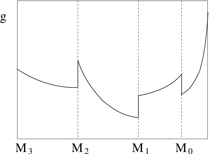
In the most simple version we use tree level matching, which means that we neglect the terms. We use this approximations throughout this work. Moreover, we use the lowest order (one-loop) beta functions for running.
We start with the symmetric linear sigma model which is parametrized at the heavy, strange mass scale in order to avoid the need for running. After the decoupling of the strange sector we are left with a model, starting at scale. The beta-functions of this model determines the running of the coupling down to , when we switch to model containing only the and mesons and the and constituent quarks. We perform in this model the running of their couplings from down to scale, where the finite temperature study is performed.
A separate treatment is needed when we treat the light masses of the system. At one hand, due to the RG running, they acquire logarithmic dependence on the heavy scale. On the other hand, because of the hierarchy problem discussed in the previous section, the light mass squared have to be fine tuned by in order to keep the light sector truely light. Therefore in bosonic models the logarithmic corrections from the RG running are subleading, and so they should be neglected.
IV Decoupling of the heavy sector
We use (1) with a background taken into account via the shift . The first step is to parametrize the heavy sector by determining the parameters of the model at scale . Then, as a next step, we perform the decoupling of the heavy (strange) sector.
IV.1 Parametrization of the heavy sector
We should fix the parameters of the heavy sector by measurements, but there exist no direct mass measurements in this regime. Therefore we are forced to make some assumptions. Since we are in a large quark mass regime, we can not use the results of the chiral perturbation theory. Instead, the heavy constituent quark model approach, where the mass of the heavy particles are simply the sum of the constituent quark masses, seems to be more adequate. In case of the light-heavy mesons this works nicely, since we can require
| (19) |
In the doubly heavy sector there is a mismatch between the scalar () and pseudoscalar () meson masses, although the constituent quark model would give the same mass for both. The reason in this model is that there is a symmetry breaking effect in addition to the constituent quark masses. To treat this situation we introduce a free parameter , and require that some average of the two mass squared is :
| (20) |
which results in a relation between the two quartic coupling constants and
| (21) |
If , i.e. when , is the smallest value for . Another plausible choice is , then . Therefore, introducing we may set
| (22) |
The parameter range will be used later in the analysis.
For fixing the other parameters we will use the infrared (IR) sector: we will determine at its own scale, this will give the mass unit in the study. For fixing the value at scale we also use an IR observable: this will be that value where we have a TCP at zero chemical potential (but, of course, at finite temperature). Through the decoupling equations this value will determine the original, zero temperature strange quark mass.
IV.2 Tree level decoupling
The next step is to eliminate the strange sector, and determine the parameters of the resulting effective model. The effective model will contain the following degrees of freedom: the upper two () components in , denoted by and the upper left submatrix in denoted by and containing the and fields:
| (23) |
We split the Lagrangian (1)-(10) according to this characterization of degrees of freedom. The shifted Lagrangian reads
| (24) |
Here, contains the heavy part, the ‘const.’ term refers to the -dependent part of the potential, while contains the terms which consist of the light fields:
| (25) | |||||
Tree level matching means that we simply neglect the heavy part, and go on with the Lagrangian described above. We can argue for this simple choice as follows. The parametrization of the heavy sector of the model could be done only very heuristically, in which case only the leading order effects could be taken into account. Therefore, it would be inconsistent to work with a detailed decoupling scheme, determining or corrections to the tree level values which are not known precisely. For this reason the leading order approach is the most consistent here. As a result of this approximation we shall trust only the most robust consequences of this study.
IV.3 Running in the linear sigma model
In component fields (25) can be written as
| (26) | |||||
where we introduced the following notations: with being the Pauli matrices, , , and The squared masses are where and (cf. (11)).
The running of the couplings are determined by the beta-functions given in Appendix A, under equation (78). By solving (78a) the running of can be obtained explicitly:
| (27) |
where . This has an UV Landau pole, while it goes to zero when .
For the other two equations, (78b) and (78c), we introduce the ratios:
| (28) |
and a new function monotonous in which satisfies
| (29) |
Using (27), this equation has the solution
| (30) |
Here we have chosen the condition , where is chosen to be the strange quark mass . Then we find:
| (31) |
Conform subsection IV.1, the phenomenologically motivated initial conditions are and at the scale of the -quark. The solution of (31) is depicted in Fig. 2.

As this plot also demonstrates, for a wide range of , stays in the interval , while decreases continuously as we lower the scale from down to . Sooner or later (depending the initial conditions) crosses zero which signals the instability of the theory. Probably it means that in order to maintain stability higher order corrections are needed.
IV.4 Running in the linear sigma model
If we are well below the scale, then we can use the model containing the sector of (26) and the constituent quarks. This model is the linear sigma model defined by
| (32) |
where and were defined in the previous two subsections. The parameters of the model are defined at scale , so we have to apply renormalization group running to find the values of the coupling at the phase transition temperature .
The RG equation are determined in Appendix B, eq. (92). The running of can be solved:
| (33) |
where This has an IR Landau pole, while it goes to zero when . The definition of is RG invariant. Comparing (33) with (27), and taking into account that the change of scaling is at we find
| (34) |
For the running of we again introduce again defined in (29) where now is the coupling of the linear sigma model. Using (33) we obtain
| (35) |
We introduce the same ratio as in (28): , and find
| (36) |
The solution of this equation reads
| (37) |
This equation has a fixed point at , as it is shown in Fig. 3

V Thermodynamics of the tricritical point
The one-loop study of the tricritical point in the linear sigma model was done in [18] using an expansion in the number of flavors. We quote below the equations (12) and (14) of that work which determine the position of the tricritical point in the plane. Using the present notation for the couplings these equations read:
| (40) |
where is the inverse temperature and with the quark baryon chemical potential. The function reads
| (41) |
This is a monotonously increasing function of its argument, .
We choose the scale , where is a number of . Then the logarithm yields , which effectively modifies . In case of spontaneous symmetry breaking , and it is useful to rescale all the masses with the tree level sigma mass at scale . Then the equations to solve will be
| (42) |
In the complete problem therefore there are 5+2 parameters: at the UV scale we have , and also we have and at the IR scale. The light mass or the corresponding is used as a mass unit. At the TCP and can be determined as functions of the UV parameters:
| (43) |
The final output of the investigation should be, of course and . But as we just have seen, even in the chiral limit of the problem is five dimensional instead of one dimensional. For a sensible prediction we have to say something about the strange mass dependence of – these functions should come from the underlying theory, now QCD. Since we do not have this information, we have to assume something sensible.
In the light of the previous subsections we make some approximations: we can fix and for we consider two cases: and The remaining function
| (44) |
can be plotted as shown in Fig. 4. The detailed numerical strategy to solve the system and obtain this plot is given in Appendix C. Fig. 4 shows surfaces in the parameter space leading to some fixed value of The critical surface is a limiting one, in the sense that surfaces with all lie on one of its side, they never cross each other. Moreover the normal vector of the surface pointing to positive always have negative component – in this sense we can say that going on the direction of the largest change, the surfaces bend downwards in .
In order to show that different values of do not change qualitatively the result we plot the surface obtained using and , and rescale the values of the latter by a factor of 1.5. The two surfaces can be seen on the right panel of Fig. 4. As the plot shows, the surfaces have the same characteristics.


V.1 Implication of the results for QCD
In real QCD we cannot change and independently. If we knew the dependence of and then we would have a curve in the space parametrized by . This line would go through the critical surfaces characterized by fix , and then we could determine the function. Since we do not have any information on the dependence of the parameters we explore several possibilities by fixing the value of one of the parameters.


For a constant value of the -dependence of the critical is shown in Fig. 5. One can see that the behavior of this curve depends strongly on how depends on . Characterized by at , there is a limiting value, and tricritical curves with smaller value of bend downwards (negative curvature), for larger values they bend upwards (positive curvature).
The standard characterization of the behavior of near is through the Taylor series [1]:
| (45) |
The first two nontrivial terms and are shown in Fig. 5 in case of a constant . The singularity corresponds to that value of the for which the curvature changes sign. It is remarkable that by changing continuously from negative to positive curvatures ( values) we have to go through a singularity.

To have a hint on which curve could be the physical one we recall that the anomaly is mainly a gauge effect, connected to the presence of the instantons [32, 33]. This suggests that The dependence of on should be quite small, so the physical line is near to . Note that all tricritical surfaces in this model with constant bend downwards.
We can compare our results with the numerical findings of [1]. They found , with degenerate quarks. The curve on Fig. 5 reproduces this value at with a corresponding value of . This is in the same order of magnitude as in the MC simulation.
In Ref. [25] it was shown that if the strength of the anomaly, parameter in the Lagrangian (10), is made -dependent then the critical surface can have a nonmonotonic shape. Since influences we can observe the same effect by considering the following dependence of on , when solving (42):
| (46) |
For most of the curves with this chemical potential dependent anomaly are very similar to what is obtained earlier, however one can observe more exotic behavior, too, for some cases. For the result is shown in Fig. 6: here the surface starts to bend upwards, and later it turns back. This behavior can be very mild (as in our example with ). In this case coarse lattice measurement would only detect the negative curvature, a high precision lattice measurement is necessary to reveal the positive curvature near . It is interesting that, considering the global behavior of the curve, the coarser lattice would give a more reliable result in this case.
VI Conclusions
We discussed the behavior of the line of tricritical points (TCP) in the chiral limit () of the quark model. We assumed that the value of the strange quark mass, where the TCP hits the line is much larger than the critical temperature . This is a good approximation in QCD, where the critical temperature is of order 160 MeV, while the constituent strange quark mass is about 450 MeV already at the physical point, and we expect that the second order line reaches the chiral line () at much higher masses. We also assumed that the meson sector, which is heavier than the sector because of the anomaly, is also much heavier than . This is again plausible, since already at the physical point GeV.
Under these circumstances the strange and the sector decouples from the point of view of the thermodynamics, which is completely determined by the light degrees of freedom, the sector. The only way how the heavy sector can influence the thermodynamics is through the values of the parameters of the effective theory. To achieve this goal we have to follow the running of the different parameters as well as the degrees of freedom from the heavy scales down to the thermodynamic scale. This can be performed by following the renormalization group (RG) flow with given degrees of freedom, and determine the parameters of the effective theories by matching when the degrees of freedom change. The former yield logarithmic dependence on the heavy scale, the latter effect is power-suppressed. Therefore in this work the RG flow is determined at one-loop level, and the matching is kept at tree level.
With the decoupling of the strange and meson sector, respectively, there are two stages of effective models in the linear sigma model: the first is the while the second is the linear sigma model. We determined the corresponding beta functions in these models, and solved the RG flow down to the scale of the temperature The thermodynamics is determined at one-loop level in [18] – we now included the running coupling constant in the result.
As a result we can determine the free energy for any given parameter sets, and we can determine those points where tricritical points (TCP) are located. With some plausible assumptions, the TCP’s with fixed (where is the quark chemical potential) form a surface in the space in the linear sigma model. Surfaces for different never cross, therefore the surface is a limiting surface.
If we want to draw consequences for QCD, we have to specify how and depend on in the chiral regime. Since it is not known, we explored several possibilities. Depending on the details, this model can describe an upward bending (positive curvature) surface or a downward bending (negative curvature) surface. Taking into account the explicit chemical potential dependence of the anomaly constant, the curvature we can change from positive to negative curvatures along the curve. In this case the value of the curvature at would yield false information about the global behavior of the curve.
Acknowledgements.
The authors benefited from discussions with András Patkós and Péter Petreczky. This work is supported by the Hungarian Research Fund (OTKA) under contract Nos. T068108 and K77534.Appendix A Renormalization group equations in the model
We start from the renormalized Lagrangian of (26), and introduce the counterterm Lagrangian which in Fourier space reads
| (47) |
where we used the shorthand and the observation that the wave function renormalization for the and sector is the same.
The goal is to determine the counterterms at one-loop level. To this end we work at zero temperature in the symmetric phase. The method is to determine the expectation value of some physical observables and require finiteness. In order to simplify the treatment we introduce a background field for the field through the shift . The expansion in is used for zero momentum external legs. The new Lagrangian is obtained from (26) reads
| (48) | |||||
where
| (49) |
with and defined below (26).
A.1 The fermionic wave function and renormalization
We calculate on the background the fermion self-energy . Introducing the notation and using standard Feynman rules we find
| (50) |
where and are the bosonic and fermionic propagators defined as
| (51) |
with the corresponding masses.
Since the integral has mass dimension, the part proportional to or are dimensionless which means that they are at most logarithmically divergent. Therefore the masses should be taken into account only through a Taylor expansion. But, the expansion in the bosonic masses yields terms, which are convergent, so we can forget about the bosonic masses. The same is true for the fermionic mass in the denominator. What remains for the divergent piece is
| (52) |
In the numerator we find which results in
| (53) |
For we have to calculate the remaining integral. Doing this with standard techniques (cf. for example [34]) using cut-off regularization we find
| (54) |
and so, the counterterm ensuring the finiteness of is
| (55) |
A.2 The bosonic wave function and renormalization
We calculate next the self-energy on the given background. We find
| (56) | |||||
The minus sign is because the fermionic bubble involves a closed fermion loop. To determine and we need only the sector:
| (57) |
After evaluating the integrals, without writing the corrections we find
| (58) |
Therefore
| (59) |
For the determination of we need the self-energy at . After evaluating the integrals we find
| (60) |
We obtain for the previous result given in (59), and we also have
| (61) |
A.3 Renormalization of
We apply the procedure above, but now for the self-energy. Since the wave function renormalization is the same as for we need only the case. We find:
| (62) | |||||
After evaluating the integrals we find for the divergent pieces
For the -mass counterterm we find he following expression
| (64) |
which is the same as the expression for the mass, with the interchange. This shows that the sum and the difference of the masses are renormalized multiplicatively: since , so we find
| (65) |
From () we can also read off the counterterm for :
| (66) |
Comparing it with the expression of given in (61) we find
| (67) |
A.4 functions
The bare-field Lagrangian reads
| (68) |
where all the fields and couplings are bare. The bare couplings are RG invariant, since they depend only on the regularization:
| (69) |
where
| (70) |
To obtain the bare quantities from the counterterms, we first have to change to renormalized fields , and :
| (71) | |||||
Comparing it with the renormalized Lagrangian defined as the sum of (26) and (47) we find and so that the relations between the bare couplings and counterterms read
| (72) |
These relations can be inverted, and at one-loop level we obtain:
| (73) |
Perturbative hierarchy requires that when there is a dependence in the quantity, then only the derivative acts on it. Then, using (70) we find
| (74) |
and in consequence
| (75) |
In a similar way we find
| (76) |
Using the expression of the counterterms determined in previous subsections of this sections we have:
| (77) |
With these expressions, we obtain from (75) and (76) the following one-loop -functions:
| (78a) | |||
| (78b) | |||
| (78c) | |||
| (78d) | |||
Appendix B Renormalization group in the linear sigma model
We start from the renormalized Lagrangian (32) and add to it the the following counterterm Lagrangian:
| (79) |
The goal is to determine the counterterms at one-loop level. To do this, we will follow the same strategy as in Appendix A. To facilitate the discussion we introduce again the background field After the shift the Lagrangian reads
| (80) | |||||
where
| (81) |
B.1 The fermion wave function and renormalization
We calculate the fermion self-energy on the background :
| (82) |
where and are the bosonic and fermion propagators introduced in (51) with the corresponding masses given in (81). Taylor expanding the bosonic propagators in and using that anticommutes with all the other gamma matrices, we find
| (83) |
After evaluating the integrals, finiteness of the result requires the following expressions for the counterterms
| (84) |
B.2 The mass, wave function and renormalization
Next, we calculate the self-energy:
| (85) | |||||
The minus sign is because the fermionic bubble. After evaluating the integrals we find, neglecting the corrections
| (86) |
Therefore, the expression of the counterterms is
| (87) |
B.3 -functions
We again use the fact that the bare couplings are renormalization group invariant:
| (88) |
where
| (89) |
This leads to:
| (90) |
Using the counterterms determined in the previous two subsections one has:
| (91) |
Then, we find the following one-loop -functions
| (92) |
Appendix C Numerical strategy to solve the TCP equations
For numerical purposes it is advantageous to choose , and as parametrization variables. Then we can proceed as follows. From (42) we find
| (93) |
then from (33)
| (94) |
Once we know and we can compute by solving equation using (39). Since now is the mass scale, in view of (39) we have to solve
| (95) |
where If we know then we can have from (33) which can be kept fixed.
References
- [1] P. de Forcrand, PoS LAT2009, 010 (2009) [arXiv:1005.0539 [hep-lat]].
- [2] Z. Fodor and S. D. Katz, arXiv:0908.3341 [hep-ph].
- [3] K. Fukushima and T. Hatsuda, arXiv:1005.4814 [hep-ph].
- [4] Z. Fodor and S. D. Katz, JHEP 0404, 050 (2004) [arXiv:hep-lat/0402006].
- [5] F. Csikor, G. I. Egri, Z. Fodor, S. D. Katz, K. K. Szabó and A. I. Toth, JHEP 0405, 046 (2004) [arXiv:hep-lat/0401016].
- [6] S. Ejiri, C. R. Allton, S. J. Hands, O. Kaczmarek, F. Karsch, E. Laermann and C. Schmidt, Prog. Theor. Phys. Suppl. 153, 118 (2004) [arXiv:hep-lat/0312006].
- [7] A. Li, “Study of QCD critical point using the canonical ensemble method,” [arXiv:1002.4459 [hep-lat]].
- [8] S. Ejiri, T. Hatsuda, N. Ishii, Y. Maezawa, N. Ukita, S. Aoki and K. Kanaya, PoS LAT2006, 132 (2006) [arXiv:hep-lat/0609075].
- [9] R. V. Gavai and S. Gupta, Phys. Rev. D 78, 114503 (2008) [arXiv:0806.2233 [hep-lat]].
- [10] C. R. Allton et al., Phys. Rev. D 71, 054508 (2005) [arXiv:hep-lat/0501030].
- [11] P. de Forcrand and O. Philipsen, PoS LATTICE2008, 208 (2008) [arXiv:0811.3858 [hep-lat]].
- [12] P. de Forcrand and O. Philipsen, JHEP 0701, 077 (2007) [arXiv:hep-lat/0607017].
- [13] P. de Forcrand, S. Kim and O. Philipsen, PoS LAT2007, 178 (2007) [arXiv:0711.0262 [hep-lat]].
- [14] P. de Forcrand and O. Philipsen, arXiv:1004.3144 [hep-lat].
- [15] R. Casalbuoni, PoS C POD2006, 001 (2006) [arXiv:hep-ph/0610179].
- [16] J. Berges and K. Rajagopal, Nucl. Phys. B 538, 215 (1999) [arXiv:hep-ph/9804233].
- [17] O. Scavenius, A. Mocsy, I. N. Mishustin and D. H. Rischke, Phys. Rev. C 64, 045202 (2001) [arXiv:nucl-th/0007030].
- [18] A. Jakovác, A. Patkós, Zs. Szép and P. Szépfalusy, Phys. Lett. B 582, 179 (2004) [arXiv:hep-ph/0312088].
- [19] E. S. Bowman and J. I. Kapusta, Phys. Rev. C 79, 015202 (2009) [arXiv:0810.0042 [nucl-th]].
- [20] P. Kovács and Zs. Szép, Phys. Rev. D 75, 025015 (2007) [arXiv:hep-ph/0611208].
- [21] P. Kovács and Zs. Szép, Phys. Rev. D 77, 065016 (2008) [arXiv:0710.1563 [hep-ph]].
- [22] B. J. Schaefer and M. Wagner, Phys. Rev. D 79, 014018 (2009) [arXiv:0808.1491 [hep-ph]].
- [23] K. Fukushima, Phys. Rev. D 77, 114028 (2008) [Erratum-ibid. D 78, 039902 (2008)] [arXiv:0803.3318 [hep-ph]].
- [24] K. Fukushima, Phys. Rev. D 78, 114019 (2008) [arXiv:0809.3080 [hep-ph]].
- [25] J. W. Chen, K. Fukushima, H. Kohyama, K. Ohnishi and U. Raha, Phys. Rev. D 80, 054012 (2009) [arXiv:0901.2407 [hep-ph]].
- [26] S. Gupta, arXiv:0712.0434 [hep-ph].
- [27] S. Gupta, J. Phys. G 35, 104018 (2008) [arXiv:0806.2255 [nucl-th]].
- [28] J. T. Lenaghan, D. H. Rischke and J. Schaffner-Bielich, Phys. Rev. D 62, 085008 (2000) [arXiv:nucl-th/0004006].
- [29] T. Herpay and Zs. Szép, Phys. Rev. D 74, 025008 (2006) [arXiv:hep-ph/0604086].
- [30] O. Philipsen, PoS LAT2005, 016 (2006) [arXiv:hep-lat/0510077].
- [31] J. Collins, Renormalization (Cambridge Monographs for Mathematical Physics, Cambridge University Press, Cambridge, UK, 1984)
- [32] G. ’t Hooft, Phys. Rev. D 14 (1976) 3432 [Erratum-ibid. D 18 (1978) 2199].
- [33] G. ’t Hooft, Phys. Rev. Lett. 37 (1976) 8.
- [34] M. E. Peskin and D. V. Schroeder, An Introduction to Quantum Field Theory, (Westview Press, New York, 1995).