Minimal resonances in annular non-Euclidean strips

In this section, we review the elasticity of swelled sheets, and establish notation for the rest of the paper. Consider an elastic sheet with thickness $t$ that has swelled by the position-dependent scalar $\Omega$. For thin sheets, the energy can be decomposed into two terms, $E=E_{C}+E_{B}$, the in-plane stretching energy $E_{C}\propto t$, and the bending energy $E_{B}\propto t^{3}$ [10, 17, 23]. This swelling factor measures the change of infinitesimal distances on the sheet, and can be converted to a “prescribed” metric tensor, $\bar{g}_{ij}$. When the actual metric (tensor) $g_{ij}$ equals the prescribed metric $\bar{g}_{ij}$, the in-plane stretching energy, $E_{C}$ vanishes. Therefore, $E_{C}$ is written in terms of a strain tensor, $\gamma_{ij}\equiv g_{ij}-\bar{g}_{ij}$. When $\Omega=1$, $\bar{g}_{ij}=\delta_{ij}$ in an appropriate coordinate system, and this recovers the standard formula for the strain of an elastic sheet [23].

It will prove convenient to consider a coordinate system $(u,v)$ in which the metric of the buckled surface takes the form

This can be compared to the metric on a flat disk $du^{2}+u^{2}dv^{2}$, where $u,v$ are the radius and polar angle in polar coordinates, respectively.

Coordinate systems of these types always exist locally and can be found by the construction illustrated in Fig. 1 (also see page 286 of Ref. [24]). First, choose an arbitrary curve on the surface to lie along $u=0$, and let $v$ be the parameter along that curve. For instance, this curve will be the center line of the strips that we consider. Curves of constant $v$ are defined to be geodesics perpendicular to the $u=0$ curve, parametrized by their arc length $u$. Curves of constant $u\neq 0$ are thus curves of fixed distance $u$ from the $u=0$ curve along that family of geodesics. Since the resulting curves are mutually orthogonal and $u$ is arc length, the metric must have the form of Eq. (1). By Gauss’s theorema egregium, the Gaussian curvature can be written in terms of the metric alone as $K=-\partial_{u}^{2}\rho/\rho$. The function $\rho(0,v)$ is determined by the metric on the curve at $u=0$. We will always choose the coordinate $v$ to be dimensionless, so that $\rho$ carries dimensions of length. Here, $\rho(u,v)dv$ is the infinitesimal length along curves of constant $u$ and the width, $w$, is the width of the strip after swelling.

To quadratic order in the strain, the elastic energy is [17]

where $Y$ is the Young’s modulus and $\nu$ the Poisson ratio of the sheet. The bending energy is given by the usual expression

where $\kappa\equiv Y/[12(1-\nu^{2})]$, $H=g^{ij}h_{ij}/2$ is the mean curvature and $K$ is the Gaussian curvature. These are both written in terms of the second fundamental form, $h_{ij}=\hat{\textbf{N}}\cdot\partial_{i}\partial_{j}\mathbf{r}$ where $\hat{\textbf{N}}$ is the unit surface normal. Couplings between $\gamma_{ij}$ and $h_{ij}$ cannot exist if the swelling is invariant under a change in surface orientation, $\hat{\textbf{N}}\rightarrow-\hat{\textbf{N}}$. We will also neglect variations of the sheet thickness with swelling.

The total energy $E=E_{C}+E_{B}$, or some variant of it, has been considered by a number of authors [4, 12, 15, 16, 14]. This functional provides a natural generalization of the usual elastic energy to non-Euclidean metrics.

Minimizing this energy is difficult because the metric and curvature tensors are not independent when a surface is immersed in three dimensions. In fact, they satisfy a set of compatibility relations, which we will briefly review in this section. To begin, we write two equations for how the frame $(\partial_{u}\textbf{r},\partial_{v}\textbf{r}/\rho,\hat{\textbf{N}})$ changes [25],

and

where

and

These follow from the definitions of the metric and second fundamental forms in our coordinates.

These two matrix equations are only compatible if $\partial_{u}\mathbf{R}_{v}=\partial_{v}\mathbf{R}_{u}+[\mathbf{R}_{u},\mathbf{R}_{v}]$, where $[,]$ is the commutator. This results in three equations relating the second fundamental form to the metric, the Gauss-Codazzi-Mainardi-Peterson equations [25],

The last equation is the theorema egregium of Gauss, and will be used to relate the function $\rho$ to the functions $h_{ij}$. Eqs. (26) and (I.2) can also be used as evolution equations to construct isometric embeddings for arbitrary $\rho$ provided that $h_{vv}\neq 0$ (see, for example, [16] and [18]).

Finally, we will find it useful in Sec. II to relate the components of the curvature directly to the mean curvature, $H$, given by $2H\equiv g^{ij}h_{ij}=h_{uu}+h_{vv}/\rho^{2}$. Using this relation in the theorema egregium, we find

Therefore $h_{vv}/\rho$ and $h_{uv}$ lie on a circle and

Here, $\alpha$ tells us how the principal curvature axes are aligned with respect to the coordinate system. For example, when $\alpha=\pi/2$, the principal curvature $H+\sqrt{H^{2}-K}$ points along the tangent vector in the $u$ direction.

In this paper, we will consider the lowest order terms of the stretching and bending energies in an expansion in powers of the ribbon width. Our procedure can be justified by a careful perturbation expansion of both the stretching and bending energies in powers of the strip width $w$, valid as long as $w\sqrt{-K}\ll 1$, where $K$ is the typical Gaussian curvature associated with the prescribed metric. This expansion also yields corrections to the strain along the center line due to the bending energy and will be explored elsewhere [22].

For our purposes, we need the following fact: as the ribbon thickness is decreased, its metric more closely agrees with the prescribed metric [17, 18]. Therefore, we will assume our strips are sufficiently thin that the strain along the center line vanishes, implying that the Gaussian curvature is equal to the prescribed curvature. From the numerics in Sec. III, the assumption of vanishing strain along the ribbon center line is roughly borne out: as the thickness decreases, the strain along the center of the strip similarly decreases. According to Fig. 7, however, the Gaussian curvature mismatch, implying strain, remains along the edge. We will see that even the condition that $K$ is isometric on the center line is only approximately true for the closed strips we are able to simulate numerically. Nevertheless, the small remaining strain leads to only small quantitive errors.

The size of this error can be estimated if we note that Eqs. (26) can be used to obtain the second fundamental form for a fixed metric. For clarity, we will suppress all dependence on $u$ unless otherwise indicated until section II.2, as all quantities in our analytical model will be evaluated on the center line at $u=0$. If we suppose that the metric deviates from the prescribed metric at the center line, we can obtain an upper bound on the strain. To do so, we suppose a form for the strain for which $\gamma_{uu}=\gamma_{uv}=0$. Then $\gamma_{vv}=\rho^{2}-\bar{\rho}^{2}$. Since the Gaussian curvature determines $\partial_{u}^{2}\rho$, $\gamma_{vv}\sim\Delta\gamma~(u/\bar{\rho})^{2}$, where $\Delta\gamma$ describes the leading order deformation of the strain. Substituting this into the stretching energy in Eq. (2), we obtain a rigorous upper bound on the stretching energy

where we have dropped a very small numerical factor depending on $\nu$. This result suggests that the magnitude of the energy in the strain can be controlled by adjusting the ribbon width or, alternatively, its thickness.

Similarly, when $K=\bar{K}$ on the center line, similar considerations show that $E_{C}\sim Ytw^{7}/\bar{\rho}^{7}\Delta\gamma^{2}$ where $\Delta\gamma$ depends on the third derivative of $\rho$ at the center line. From Gauss’ theorem egregium, this is linked to derivatives of the curvature with respect to $u$.

We will approximate the bending energy by its leading order power of $w$, which should be valid when $w$ is sufficiently small. For the bending energy, this yield

where the factor of $w$ accounts for the integral over $u$. Thus, using Gauss’ theorem egregium again, this only depends on $\partial_{u}^{2}\rho$ along the center line.

This suggests that the lowest order terms in the energy are minimized when the curvature along the center line minimizes Eq. (30) subject to the constraint on the Gaussian curvature. The higher-order terms

This type of approximation has also been used to describe narrow developable strips. For instance, to obtain the Sadowsky functional [27], we would minimize Eq. (30) subject to the constraint that $K=0$ on the center line. In Sec. III, we will compare our results to a numerical minimization of several closed strips. This will both justify our assumptions as well as confirm the predictions obtained from our calculations.

For infinitely thin open strips of sufficient narrowness, it is possible to find an isometric immersion such that both $H=0$ and $\partial_{u}H=0$ along the center line [26]. Most of our numerical strips do not even have $H=0$ on the center line; in fact, we will derive conditions in Sec. II under which it is possible to at least ensure that $H=0$ on the center line.

Closed strips cut from an unswelled, flat disk have a natural coordinate system $(r,\theta)$, where $\theta$ is the azimuthal angle around the strip. In the swelled case, it is natural to force the coordinate $v$ to be $2\pi$-periodic as well. Once we determine $\rho$, $\partial_{u}\rho$, $\partial_{u}^{2}\rho$, and $h_{ij}$ on the center line at $u=0$ that result in a closed strip, Eq. (I.2), which governs the evolution along lines of constant $v$, will preserve the periodic structure of the strip away from the center line.

We first note that Eq. (I.2) determining the evolution of the strip frame along $v$ can be recast as an equation for the components of the two tangents and the surface normal in space along the center line. Taking the $x$-component,

Similarly, we can replace $\hat{x}$ with $\hat{y}$ or $\hat{z}$. The skew-symmetric matrix $\textbf{R}_{v}$ is an infinitesimal rotation that depends on the second fundamental form along the strip center line, which itself is a function of $v$. Therefore, Eq. (II.1) can be recast as the equation for a particle in a magnetic field. To make this mapping explicit, we identify the $v$ coordinate with time and define a “time-dependent magnetic field”

and the vector

The index on $\mathbf{v_{x}}$ refers to the fact that it arises from taking the $x$-component of the frame in Eq. (II.1). The curves $\mathbf{v_{y}},\mathbf{v_{z}}$ are defined similarly. The $\hat{i},\hat{j},\hat{k}$ introduced here label the $\partial_{u}\textbf{r}$, $\frac{\partial_{v}\textbf{r}}{\rho}$, and $\hat{\textbf{N}}$ components in the frame in Eq. (II.1) and are not the directions $\hat{x},\hat{y},\hat{z}$ of our three dimensional Euclidean space. Eq. (II.1) now reads

So far, the steps we’ve taken here in no way restrict the generality of our discussion. Requiring that our surface is a closed strip is equivalent to finding conditions on B such that $\mathbf{v_{i}}(v)$ is a closed curve and that $\int_{0}^{2\pi}\rho(v)~[{\bf v_{i}}(v)\cdot\hat{j}]dv=0$ for $i=x,y,z$. Supposing this could be done, the problem would be to minimize the energy with respect to $h_{ij}$ and $\rho$ on the set of all closed solutions. However, this is related to the open Fenchel problem of finding conditions on the curvature and torsion of a space curve in order for it to close. Instead of finding all possible closed solutions, we will construct an ansatz for a class of solutions that admit a relatively simple characterization.

We will restrict ourselves to strips whose normal vector, on the center line, is constrained to lie on a cone. For convenience, we will refer to these as “conical strips.” Though our motivation for considering these solutions was originally to simplify our analysis, this choice of ansatz turned out to be particularly apt, as will be shown in Sec. III. In appendix A, we derive expressions for conical strips with general mean curvatures along the center line. We summarize the results and notation here. First, we define $\sin\xi=H/\sqrt{H^{2}-K}$ and recall that $H=h_{uu}+h_{vv}/\rho^{2}$ and $K=-\partial_{u}^{2}\rho/\rho$ on the center line from Sec. I.2. We also have the angle $\alpha$ between the principal curvature axes of the strip and the axes of the $uv$ coordinate system.

The final result for the tangent vector of the center line of the strip is

with a constant cone angle $\phi$ between $\hat{\textbf{N}}$ and $\hat{z}$, satisfying

with $W(v)=\sec\phi\int_{0}^{v}dv^{\prime}[\partial_{v^{\prime}}\beta(v^{\prime})-\partial_{u}\rho(v^{\prime})]+W_{0}$, where $W_{0}$ is an arbitrary constant, and $\tan\beta=(\sin\alpha-\sin\xi)/\cos\alpha=h_{vv}/(\rho h_{vu})$. These expressions can be written directly in terms of the functions $\rho$ and $h_{ij}$ that characterize the shape of the strip on the center line.

We now derive conditions under which a conical strip closes. We first note that the tangent vectors can only be periodic if $\Delta\beta\equiv[\beta(2\pi)-\beta(0)]/(2\pi)$ and $\Delta W\equiv[W(2\pi)-W(0)]/(2\pi)$ are integers. Note that if we fix $0<\phi<\pi/2$ then the magnitude of the term with $\cos^{2}(\phi/2)$ in Eq. (42) is larger, so that the number of times the strip wraps around will be set by the period of $W-\beta$ rather than $W+\beta$. Therefore, we interpret $\Delta W-\Delta\beta$ as the number of times the strip wraps around the $z$-axis. In particular, this implies that if we were to cut a closed strip from the edge of a disk, we should require $\Delta W-\Delta\beta=\pm 1$; other choices of $\Delta W-\Delta\beta$ could be used to represent knotted strips. In addition, the integer $\Delta\beta$ counts the number of times that the tangent vector of the center line crosses the $z=0$ plane, since it does so whenever $\beta$ is an odd integer multiple of $\pi/2$. Therefore, we interpret $\Delta\beta$ as the number of wrinkles of a closed strip. Finally, we define $\Delta\rho\equiv[\int_{0}^{2\pi}dv~\partial_{u}\rho(v)]/(2\pi)$. From the definition of $W$,

and thus the two choices of $\Delta W$ for a given $\Delta\beta$ mean that we have two possible cone angles $\phi$ for a given metric that can lead to closed conical strips. This gives us a criterion for the existence of such a strip, since $\Delta\rho$ and $\Delta\beta$ must be chosen so that $0<\cos\phi<1$ (since $0<\phi<\pi/2$). In particular, this implies

The above conditions ensure that $\partial_{v}\textbf{r}/\rho$ is periodic. As a final constraint, $\partial_{v}\textbf{r}$ must integrate to zero as $v$ goes from 0 to $2\pi$ to ensure that r is periodic as well.

It is instructive to consider some specific examples to understand the formulas derived in the last section. Consider first conical strips with $\Delta\beta=0$. This class of shapes contains all of the axisymmetric strips, for which $\beta$ is constant in $v$. With this, $0<\Delta\rho<1$. For axisymmetric strips, for which $\rho$ is also independent of $v$, this criteria is well-known (see the proof in Marder et al. [28] for another derivation of this criteria for axisymmetric strips). The class of strips with $\Delta\beta=0$ contains, but is not limited to, axisymmetric shapes – the function $\beta$ need not be constant; all that is required is that $\beta$ be periodic as $v$ varies from $0$ to $2\pi$. The condition $0<\Delta\rho<1$ yields a limit on how quickly $\rho$ can grow with $u$ for such a conical strip. This has ramifications for a disk with $K=-1/R^{2}$, which has a metric with $\rho(r,v)=R\sinh(u/R)$ [9, 18], where $r$ is the radial distance from the disk center. If we imagine cutting a narrow strip from the edge of the disk with center line at $r=u_{0}$, $\partial_{u}\rho=\cosh(u_{0}/R)>1$, which violates the constraint for $\Delta\beta=0$.

We next turn our attention to the case of $\Delta\beta=2$, corresponding to a saddle shape in which $h_{0,vv}$ has four zeros (two wrinkles). Then solution in this class of strips must have $1<\Delta\rho<2$ or $-1<\Delta\rho<2$. If we specialize again to a strip cut from a constant negative Gaussian curvature disk so that $\rho(u,v)=R\sinh((u+u_{0})/R)$, $\rho=R\sinh(u_{0}/R)$ and $\Delta\rho=\cosh(u_{0}/R)$, and we find that a solution of the first type is possible when $0<u_{0}<R\cosh^{-1}(1)$ or $0<u_{0}<1.32R$. At the limiting case, $\cos\phi=0,1$ and the mean curvature along the center line diverges, as can be readily seen from Eq. (62).

However, this should not be interpreted as the maximum radius of finding a saddle-shaped isometric embedding. In fact, arbitrarily large isometric embeddings of disks with $K=-1/R^{2}$ exist [20]. If we were to cut a strip from the edge of such an isometric embedding with radius larger than $R\cosh^{-1}(2)$, the strip center line may still have two wrinkles (alternatively, four zeros for $h_{vv}$). It could not be a conical strip, however. Consequently, it is likely that minimal energy strips deviate from the shapes we would predict for conical strips, especially when the mean curvature is large.

We now return to conical strips with $H=0$ along their center line. In that case, using Eq. (62), we have

at every $v$. For simplicity, we will specialize to the case that $\rho$ is constant in $v$ along the center line, though by replacing these quantities by their averages over $v$ we could lift this specialization. In this case, $\Delta\rho=\partial_{u}\rho$ which implies that $\partial_{v}\beta=\Delta\beta$. Squaring both sides and using $\cot^{2}\phi=\frac{\left(\Delta\beta-\Delta\rho\right)^{2}}{\left(\Delta\beta\pm 1\right)^{2}-\left(\Delta\beta-\Delta\rho\right)^{2}}$ derived from Eq. (44), we find

which implies

Consider again the disk with constant negative gaussian curvature $-1/R^{2}$. For a strip with center line at radius $u_{0}$, $\rho=R\sinh(u_{0}/R)$, $\partial_{u}\rho=\cosh(u_{0}/R)$, $\partial_{u}^{2}\rho=\rho/R^{2}$ and the resonance condition above is satisfied when $\Delta\beta=\cosh(u_{0}/R)\mp 1$. This generalizes the condition found by one of us numerically [18]. For the class of solutions considered there, this condition could also be derived by Fourier analysis.

Again, it need not be the case that there are no closed strips with $H=0$ along their center lines when this condition is not satisfied, only that there are none in the class of closed, conical strips. Nevertheless, our results do have ramifications on the shape of minimal energy strips: we will see in the next section that we can satisfy both the bending and stretching energies to lowest order in powers of $w/R$ at one of these resonances. Therefore, in the regime of thickness we are primarily concerned with in this paper, $\partial_{v}\beta=\cosh(u_{0}/R)\mp 1$ is sufficient to demonstrate that $H=0$ along the center line. The numerical evidence we will present in Sec. III suggests that, at the very least, embeddings with zero mean curvature on the center line do not exist for all choices of metric.

We now seek to minimize the bending energy along the center line of a closed, conical strip. The energy in Eq. (30) would be minimized when $H=0$ along the center line. Happily, such a condition can be satisfied within the class of closed, conical strips when Eq. (48) is satisfied. In this section, we are interested in the minimal energy shape close to $H=0$ as well.

When $H=0$ along the center line, $\beta=mv$ from Eq. (46). Near an $H=0$ resonance, we can look for an approximate minimum of the form $\beta=mv+f$, where $\beta=mv$ is the solution for the $H=0$ strip with $m$ wrinkles. Using Eq. (62), we expand $H$ in powers of $f$ to find

This allows us to expand Eq. (30) to quadratic order in $f$, from which we find the Euler-Lagrange equation

which has solution

where $A$ is a constant independent of $v$. Looking at Eq. (62) for the mean curvature, we see that $\partial_{v}\beta$ always appears in the combination $\partial_{u}\rho-\partial_{v}\beta$. Therefore, we can interpret the first term of Eq. (51) as a shift in $\partial_{u}\rho$, which must be accompanied by a $v$-dependent correction proportional to $\sin(2mv)$. Therefore, when $\partial_{u}\rho$ is tuned away from a resonance by an amount $A/2$, the function $\beta$ oscillates with a frequency $2m$.

We can use this near-resonance solution as the basis for a general conical strip ansatz valid for all metrics: $\beta=mv+\tilde{A}\sin(2mv)/(2m)$. For sufficiently small $\tilde{A}$, this ansatz does not modify the location of the zeros of $\sin\beta$ nor does it alter $\partial_{v}\beta$ at those zeros. It is straightforward to show that the zeros of $h_{vv}$ coincide with those of $\sin\beta$. At those zeros, $\partial_{v}\beta=m-\tilde{A}$. For $H$ to remain finite at those zeros, inspection of Eq. (62) implies that $\partial_{v}\beta=\partial_{u}\rho+\cot\phi\sqrt{\rho\partial_{u}^{2}\rho}$ when $\sin\beta=0$. Therefore, we conclude that $\tilde{A}=\partial_{u}\rho+\cot\phi\sqrt{\rho\partial_{u}^{2}\rho}-m$.

Finally, it is necessary to confirm that this ansatz yields a closed strip. Since $\partial_{u}\rho$ is independent of $v$, $W=\sec\phi[\partial_{u}\rho~v-\beta(v)+\beta(0)]+W_{0}$. Examining the form of $\beta$, both $W$ and $\beta$ change sign when $v\rightarrow v+\pi/m$. Inserting this into the equation for the tangent vector and integrating, we find that $\int_{0}^{2\pi}dv~\rho~\partial_{v}\mathbf{r}/\rho=\mathbf{r}(2\pi)-\mathbf{r}(0)=0$.

To summarize the construction in this section, assume that we are given some $\rho(u,v)$. We would like to construct an ansatz with $m$ wrinkles. Next, we calculate $\tan\phi$ using Eq. (44). There are two choices, which are perhaps not equally good. Once this choice is made, it is straightforward to calculate $A$, $\beta$, $W$ and then we have the expressions for the frame on the strip, including Eq. (42) for the tangent vector as well as the other components, whose expressions are in Appendix A. If we integrate the tangent vector, we may generate the space curve of the center line. To construct the surface, we integrate Eq. (I.2) in a small neighborhood of the center line. We depict center lines of strips with $m=3,4,5$ in Fig. 2.

To corroborate our analysis, we have implemented the bead-and-spring model of inhomogeneous swelling developed by Marder and Papaniolaou [16]. An unswelled sheet is represented by a stacked pair of close-packed triangular lattices with a periodic length of 200 beads and a width of 20 beads (thus, 8000 particles). Nearest neighbors in the lattice are connected by harmonic springs (35000 total bonds) with bond energy between two lattice sites $a$ and $b$ given by

where $|\Delta\mathbf{X}|$ is the bond length. The swelling is incorporated by setting the equilibrium bond length according to the approximate equation

where $\Delta x^{i}$ are the components of the vector connecting beads $a$ and $b$ in the unswelled membrane and $\bar{g}_{ij}$ is the prescribed metric. This approximates the integral that measures the prescribed distance between points $a$ and $b$. The prescribed metric used in Eq. (53) is given by the average of the continuum prescribed metric evaluated on the lattice points $a$ and $b$. Alternatively, we could evaluate the continuum prescribed metric somewhere along the bond; as long as the average bond length is small compared to $R$, the details of how we evaluate the prescribed length between neighboring points $a$ and $b$ do not change our results.

As shown in Ref. [16], Eq. (52) is compatible with a continuum limit using the strain $\gamma_{ij}=g_{ij}-\bar{g}_{ij}$. Note that the 2D strip energy consisting of a sum of stretching and bending energies is recovered from this 3D model when the thickness is small. In particular, we note that the bending energy arises naturally from the differential stretching and compression of the two layers of the sheet. The energy is minimized using either a conjugate-gradient or Broyden-Fletcher-Goldfarb-Shanno (BFGS) algorithm, as implemented the GNU Scientific Library (GSL). In general, we find that strips develop “creases” often as the minimization procedure proceeds unless the strips are sufficiently thick and the change in the degree of swelling sufficiently small. As a practical matter, therefore, we start our minimization with thick strips, $t\approx 0.025w$, and small prescribed curvatures $\bar{K}\approx-10^{-2}w^{-2}$. We then increase the curvature in a sequence of steps to the desired curvature (up to $\sqrt{\bar{K}}w\approx 1.3$) and, once this sequence is complete, decrease the thickness to the desired thickness (down to $t\approx 0.004w$). If we decrease the thickness first, the strips often develop creases, though as long as the strips remain smooth during this process, the energy minima we have found appear to be quite robust against changes in the sequence of steps taken. Finally, it is difficult to maintain a smooth strip shape, even at fixed swelling, once the thickness becomes too small. Therefore, we are not able to probe the limit of truly thin strips; consequently, all our strips seem to have some residual strain, even in the ground state.

We find that strips with different numbers of wrinkles are metastable, and have explicitly seen this up to five wrinkles. Therefore, to select the number of wrinkles, we bias the minimization by choosing an initial strip shape with a prescribed number of wrinkles $m$. Typically, we use the graph $z(r,\theta)=h_{0}\cos(m\theta)$ as an initial condition for the lattice, where $r$ and $\theta$ are polar coordinates in the $xy$ plane. We have also tried adding additional Fourier modes in the initial conditions and have tried amplitudes in the range $0.01t<h_{0}<100t$ for sheets of thickness $t$. In all cases we have tried, the number of wrinkles is primarily chosen by the dominant mode in $z(r,\theta)$, though there is a small bias toward lower energy structures with two wrinkles, and all strips with the same number of wrinkles are nearly identical. If no bias is chosen, the minimization will take a long time to break the symmetry and will go into a state with two or three wrinkles.

Finally, since we are interested in verifying the assumptions and predictions of our analytical calculations here, we will focus on metrics with $\rho(u,v)$ independent of the longitudinal direction $v$. We have explored two prescribed metrics in detail: (1) $\rho_{1}(u,v)=R\sinh(u/R+u_{0}/R)$ and (2) $\rho_{2}(u,v)=R\cosh(u/R)/(2\pi)+\eta R\sinh(u/R)$. Both of these metrics have $K=-1/R^{2}$ everywhere. The first of these corresponds to cutting a strip of width $w$ from the edge of a buckled disk at radius $u_{0}-w/2$. The resonance condition for the center line of this metric gives $\cosh(u_{0}/R)=m-1$. For $m=3$, this requires a degree of swelling which is difficult to achieve numerically at low thicknesses. Therefore, to study the resonance condition numerically, we use $\rho_{2}(u_{0})$ for various values of $\eta$. From the resonance condition in Eq. (48), we have four solutions

where the $\pm$ must be chosen consistently in each equation. With the swelling factors accessible to our numerics, we are able to probe the branch of resonances with $\eta$ near $+1$ for $2$, $3$, and $4$ wrinkles.

Geometric quantities such as $H$, $K$ for our numerically minimized surfaces are computed from an interpolation of the points on the mid-surface between the two bead-spring sheets.

As an example of a minimial energy surface from our numerical calculations, Fig. 3 shows a four wrinkle strip with metric from $\rho_{1}$ and $t=0.01w$ with prescribed Gaussian curvature, $\bar{K}=-(1/9)w^{-2}$. In Fig. 4, we plot the Gaussian curvature along the center line for strips for three thicknesses $t/w=0.02$, $0.015$, and $0.01$ and otherwise identical parameters. As expexted, along the center line $K$ approaches its prescribed value as the thickness decreases. It is interesting to note that even for the thinnest strips we have tried, the Gaussian curvature always displays localized regions of stretching. Nevertheless, our results are apparently robust against this localized residual strain.

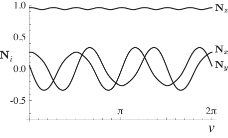
In Fig. 5, we plot the three components of the normal vector on the center line for the thinnest of the strips in Fig. 4. The $x$ and $y$ components oscillate (with amplitude close to $0.25$) around zero while the $z$ component is very nearly constant. To quantify this, we compute the average $N_{z}\equiv\langle\mathbf{N}\cdot\hat{z}\rangle\approx 0.950$ and the variance $[\langle(\hat{N}\cdot\hat{z}-N_{z})^{2}\rangle]^{-1/2}\approx 0.01$. The analytical angle $\cos\phi$ is predicted from Eq. (44) to be $0.951$.

Similar levels of agreement are obtained for other choices of metric, curvature and thicknesses, though thinner sheets have a closer agreement. We tested 2-, 3-, and 4-wrinkle strips of thickness $t/w=0.025$ with metric from $\rho_{1}$ (with $u_{0}/w=5/\pi$ as are all strips with $\rho_{1}$ in this paper) starting from $R=150$ and increasing the curvature down to $R\approx 20$. Fig. 6 shows the resulting average $\cos\phi$ on the center line as a function of $\partial_{u}\rho=\cosh(u_{0}/R)$, where the error bars show the variance of $\cos\phi$. Our theory and Eq. (44) predict a linear relationship, with zero variance. This is observed up to fairly high curvatures – at the curvatures where $\cos\phi$ begins to oscillate, we observe an intriguing symmetry-breaking from strips with $D_{md}$ symmetry to strips with $C_{mv}$ symmetry, and the wrinkles curl into tubes. The explanation of this transition is outside the scope of this paper, but we display this transition in 2-wrinkle strips in the inset of Fig. 6. We note that in this symmetry-breaking transition, as in the minimization without a bias towards a set number of wrinkles, the system seems to take a long time to find a minimum, often oscillating between different states.

In Fig. 7, the distribution of Gaussian curvature is plotted for three thicknesses ($t/w\approx 0.008$, $0.004$ and $0.0015$) and $\bar{K}w^{2}=-0.029$ for prescribed metric $\rho_{1}$. A boundary layer is evident in all the images. In both cases the degree of stretching decreases near the center of the strip as the thickness decreases.

We further test our model by comparing the numerically obtained $H$ along the center line with our analytical calculations. In Fig. 8, we show the specific case with prescribed metric $\rho_{1}$, $t/w=0.006$ and $\bar{K}=-0.029$. The solid lines show $H/\sqrt{|\bar{K}|}$ along the center line for strips with different numbers of wrinkles from $m=2$ to $m=5$. For the purposes of comparison, we rescale $v$ to contain one period of the strip, $2\pi/m$. Though these curves agree favorably in magnitude with those predicted by our theory, there is some discrepancy in the precise strip shape. This discrepancy may be caused by the failure of the Gaussian curvature to agree with the prescribed curvature exactly or perhaps by the fact that the analytical center line may approximate a curve on the strip that is not exactly in the center.

A more stringent test of the analytical theory is the surprising resonance condition of Eq. (48). Since resonances are at relatively high curvatures it is more difficult to achieve low thicknesses without creases using metric $\rho_{1}(u)$, we focus on the metric $\rho_{2}(u)$ with various values of $\eta$. We choose $t/w=0.00375$ and $\bar{K}w^{2}=-0.01$; though very thin, even at this $t/w$ there is some deviation of $K$ along the center line from its prescribed value. In Fig. 9, we show the numerically measured variance of mean curvature and the analytical predictions from the ansatz in Sec. II.3 for such strips. It is clear that the shape of the variance as a function of $\eta$ is fairly well-mimicked with $\eta$ above resonance, but there is less good agreement below resonance. In fact, the numerically minimized shapes tend to look nearly flat at $\eta=1$, as opposed to the ansatz which predicts a singular strip. For completeness we include Fig. 10 which shows this data for the $\rho_{1}$ strips shown in Fig. 6 – the agreement appears to be worse as a result of the thickness being around $t/w=0.025$. It does appear for 3-wrinkle ribbons that the point at which the numerical data begins to differ from the predictions occurs near the same values of $\partial_{u}\rho$ where the symmetry-breaking transition causes the conical strip ansatz to fail.

For 2-wrinkle strips, at $\eta\approx 1.0055$ and $\eta\approx 1.0010$ below resonance we observe fairly sharp and reproducible jumps in the variance of the mean curvature – we do not currently have a good explanation of this, as the strip shapes do not appear to change dramatically over these values of $\eta$.

In Fig. 11, we plot $\langle H^{2}(u)/H_{0}^{2}\rangle=\int dv~\rho(u)[H^{2}(u,v)/H_{0}^{2}]/[2\pi\rho(u)]$ over the surface of numerically minimized strips with two, three, and four wrinkles above, near, and below resonance. Here $H_{0}$ is the average mean curvature in a certain region of the strip. There is a clear trend toward extinguishing the mean curvature near the center line of the strip when $\eta$ is tuned near the resonance condition of Eq. (48).

Eq. (48) and its application to $\rho_{2}$ strips, Eq. (56), predicts rather well the observed location of the resonance. We find that the center line of a two wrinkle strip will have $H=0$ when $\eta\approx 1.01275$, a three wrinkle strip will have $H=0$ when $\eta\approx 1.00634$, and a four wrinkle strip will have $H=0$ when $\eta\approx 1.00422$.

For example, with two wrinkle strips we find that the mean curvature is slightly smaller with $\eta=1.012$ than near the predicted resonance of $\eta=1.013$. We ascribe this small discrepancy to our assumption that the Gaussian curvature along the center line agrees with that prescribed by the metric. Indeed, thick membranes do not show any evidence of the resonance condition at all, nor does the Gaussian curvature reach its prescribed curvature on the center line. It is also interesting to note that, below resonance, the mean curvature near the center line of a strip is $\pi$ out of phase with the mean curvature near the strip edges.

Finally, we plot the energy for $\rho_{1}$ and $\rho_{2}$ in Figs. 12 and 13. In both cases, the energy of $m=2$ appears to be lowest throughout the range of parameters tested, though for a large degree of swelling the energies become nearly degenerate. For Fig. 13, dips in the energy occur at the resonances in $\eta$ as we might expect, since the dominant term in the bending energy vanishes near the resonances. In Fig. 12, the resonances occur in the regions where $R$ is small and the energies are nearly degenerate. At large $R$, the energy scales as $1/R^{2}=|\bar{K}|$, which we expect since $E_{B}\sim H^{2}\propto 1/R^{2}$.

Note that, at a resonance, the energy is dominated by higher order terms that we have neglected in our analysis. It is these additional terms that set the energy scale at the resonances. It is these higher order terms that seem to determine which shapes have the lowest absolute energy.

References

- [1] D. Drasdo, Phys. Rev. Lett. 84, 4244 (2000).
- [2] H. Liang and L. Mahadevan, Proc. Nat. Acad. Sci. 106, 22049 (2009).
- [3] M. Marder, Found. Physics 33, 1743 (2003).
- [4] E. Sharon, B. Roman and H.L. Swinney, Phys. Rev. E 75, 046211 (2007).
- [5] U. Nath, B.C.W. Crawford, R. Carpenter and E. Coen, Science 299, 1404 (2003).
- [6] A. Goriely and M. Ben Amar, Phys. Rev. Lett. 94, 198103 (2005).
- [7] E. Sharon, B. Roman, M. Marder, G.S. Shin and H.L. Swinney, Nature (London) 419, 579 (2002).
- [8] T. Mora and A. Boudaoud, Eur. Phys. J. E 20, 119 (2006).
- [9] Y. Klein, E. Efrati, and E. Sharon, Science 315, 1116 (2007).
- [10] L.D. Landau and E.M. Lifschitz, Theory of Elasticity, 3rd Ed. (Pergamon, London, 1959).
- [11] J. Dervaux and M. Ben Amar, Phys. Rev. Lett. 101, 068101 (2008).
- [12] S. Nechaev and R. Voituriez, J. Phys. A 34, 11069 (2001).
- [13] B. Audoly and A. Boudaoud, C.R. Mecanique 330, 831 (2002).
- [14] B. Audoly and A. Boudaoud, Phys. Rev. Lett. 91, 086105 (2003).
- [15] M. Marder, E. Sharon, S. Smith, and B. Roman, Europhys. Lett. 62, 498 (2003).
- [16] M. Marder and N. Papaniolaou, J. Stat. Phys. 125, 1065 (2006).
- [17] E. Efrati, E. Sharon, R. Kupferman, J. Mech. Phys. Sol. 57, 762 (2009).
- [18] C.D. Santangelo, EPL 86, 34003 (2009).
- [19] Q. Han and J-X. Hong, Isometric Embedding of Riemannian Manifolds in Euclidean Spaces, Mathematical Surveys and Monographs, vol. 130 (American Mathematical Society, Providence, RI , 2006)
- [20] E.G. Poznyak and E.V. Shikin, J. Math. Sci. 74, 1078 (1995).
- [21] J. Gemmer and S. Venkataramani, e-print arXiv:1005.4442
- [22] B.G. Chen and C.D. Santangelo, (unpublished).
- [23] P.G. Ciarlet, J. Elasticity 78-79, 1 (2005).
- [24] M.P. Do Carmo, Differential Geometry of Curves and Surfaces, (Prentice-Hall, Englewood Cliffs, NJ, 1976).
- [25] D.J. Struick, Lectures on Classical Differential Geometry, 2nd ed (Addison-Wesley, Reading, Mass, 1961).
- [26] E. Efrati, E. Sharon and R. Kupferman (private communication).
- [27] M. Sadowsky, Sitzungsber. Preuss. Akad. Wiss. 22, 412 (1930).
- [28] M. Marder, R.D. Deegan and E. Sharon, Phys.Today 60(2), 33 (2007).
- [29] E. Sharon, private communication (2010).