Discontinuous Transition in a Boundary Driven Contact Process
Abstract
The contact process is a stochastic process which exhibits a continuous, absorbing-state phase transition in the Directed Percolation (DP) universality class. In this work, we consider a contact process with a bias in conjunction with an active wall. This model exhibits waves of activity emanating from the active wall and, when the system is supercritical, propagating indefinitely as travelling (Fisher) waves. In the subcritical phase the activity is localised near the wall. We study the phase transition numerically and show that certain properties of the system, notably the wave velocity, are discontinuous across the transition. Using a modified Fisher equation to model the system we elucidate the mechanism by which the the discontinuity arises. Furthermore we establish relations between properties of the travelling wave and DP critical exponents.
1 Introduction
The contact process [1] exhibits a nonequilbrium phase transition from an absorbing state, where the system ends up in an inactive configuration, to an active, fluctuating state. Although originally introduced as a microscopic model for epidemic spreading, this lattice model and its relatives have been used to describe a variety of systems including percolation, wetting, reaction-diffusion processes, branching and annihilating random walks [2] and phase transitions in more exotic settings, such as between two turbulent states in nematic liquid crystals [3], and in proliferating microbial populations under gravity [4]. The continuous phase transition from the inactive to active phases falls into the Directed Percolation (DP) universality class which is thought to pertain for any such microscopic model exhibiting an absorbing state phase transition, in the absence of any additional symmetries or conservation laws [5, 6].
The nature of the transition may be modified by the introduction of an active boundary into the system that ensures that the activity in the system never dies out [7, 8, 9, 10]. These studies have mainly focused on surface critical behaviour and the emergence of new surface critical exponents. In the counterpart to the inactive phase the activity is confined to the boundary region whereas in the counterpart to the active phase the activity spreads from the boundary through the system. The spreading of activity through the system from the boundary is conveniently illustrated in the mean-field description of the DP universality class [2] which has the same form as the Fisher-KPP11 1 Here Fisher-KPP stands for Fisher-Kolmogorov-Petrovskii-Piskunov. It is alternatively called the Fisher-Kolmogorov or Fisher equation. equation [11]. This nonlinear partial differential equation exhibits travelling wave solutions in which the active phase invades inactive regions with a well-defined velocity for the domain wall that separates the two regions.
In this work we consider a variation of the contact process with the two features of an active boundary and advection away from the boundary which we refer to as the Driven Asymmetric Contact Process (DACP). The Asymmetric Contact Process has been previously studied in the absence of boundaries and yields a phase transition in the DP universality class, as expected [12, 13, 14]. The addition of an active boundary, which serves to drive the system, then modifies the nature of the transition as described above [9]. However, what we discover is that the DP transition now has a discontinuous aspect in the sense that the velocity of the wavefront which carries the activity from the boundary jumps discontinuously at the critical point. Thus, intriguingly, the continuous DP transition is accompanied by a velocity discontinuity in the presence of an active boundary and advection.
There has been recent interest in the addition of an advection term to the Fisher-KPP equation in the presence of a boundary since a Galilean transformation no longer serves to remove the advection term (as would be the case in the absence of boundaries). When the advection is directed towards the boundary there is a competition between the advective velocity and the Fisher wave velocity, leading to a phase transition [4, 15, 16] from a phase with activity localised near the boundary to one where the Fisher wave invades the whole system. The addition of noise into this system leads to a more complicated scenario where, in the case of a reflecting boundary studied in [17], the low activity phase could either be localised near the boundary or be the absorbing state. However, the discontinuous transition observed in that work where the bulk density jumps at the transition, is distinct from that studied in the present work.
To understand the transition we observe, we consider a phenomenological mean-field description of the system in the form of a Fisher-KPP equation which includes the effects of asymmetry in the form of an advective term. We show that the solution can be thought of as a Fisher wave moving within an envelope given by the stationary density profile. Thus, in the subcritical regime the system exhibits attenuated waves with non-zero velocity but whose amplitude decays to zero away from the boundary. In the supercritical regime, on the other hand, the stationary profile has a non-zero limit far from the boundary, thus the Fisher wave propagates into the bulk with a constant amplitude and non-zero velocity. This is the mechanism for the observed discontinuity of the velocity.
The paper is organised as follows: In section 2 we define the microscopic model and in section 3 we present numerical evidence for the discontinuous phase transition. In section 4 we discuss the observed scaling behaviour and identify the Directed Percolation critical exponents. In section 5 we discuss a mean field theory in the form of a modified Fisher-KPP equation. Using the mean field picture we then re-examine in section 6 the simulation results to show that a similar picture holds. We conclude in section 7.
2 Microscopic model
The driven asymmetric contact process (hereafter, DACP) is a stochastic model defined on a one-dimensional lattice. A microscopic configuration is specified by the set of occupation numbers where indicates that site is inactive (active) at time . The leftmost site of the system is kept permanently active, , making the process driven. Active sites can activate inactive sites directly to the right of them at rate or become inactive with rate 1. See Fig. 1 for an illustration.
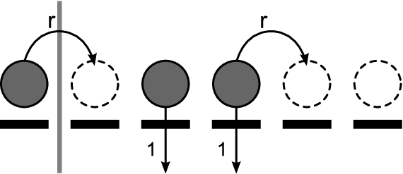
The driving from the left boundary eliminates the absorbing state associated with the basic contact process. However as the rate goes through a critical value there is still a continuous phase transition from a phase where the active sites can only spread a finite distance from the left boundary to a phase where they can spread to infinity. See Fig. 2 for an illustration of the density profile in the two states.

An interesting and attractive feature of the model is that the total asymmetry of the activation dynamics means that the state of site is independent from that of for . This implies that any calculation or simulation performed on a finite system of sites gives the exact behaviour for the first sites of an infinite system. In other words, the introduction of a right boundary does not introduce any finite-size effects.
We now summarise previous work on asymmetric contact processes. Three mathematical papers [12, 13, 14] have looked at how introducing asymmetry into the contact process (without a boundary drive) leads to the emergence of a second order parameter, the probability that the origin is active as , in addition to the probability that the process remains active indefinitely. At total symmetry the two order parameters coincide and at total asymmetry the second disappears. An approximate analytical and numerical study of the totally asymmetric contact process (without a boundary drive) [18] found a continuous transition at the critical rate with the critical exponent which is in agreement with the value for the DP order parameter exponent in one spatial dimension. In addition a two-dimensional generalisation of the DACP was constructed [9] and used to study wetting and interface phenomena [19].
3 Numerical evidence for a discontinuous velocity transition
We begin our study of the DACP by presenting numerical data that suggests the velocity of the wave emanating from the left boundary is discontinuous at the phase transition point.
3.1 Simulation details
We performed direct Monte Carlo simulations of the microscopic DACP dynamics specified in section 2 above. Each run was initialised with the lattice unoccupied, apart from the 0th site which is kept permanently active. During the simulation a list of active sites is maintained. In each elementary update, one of the active sites is chosen from this list at random. With probability , its right neighbour is activated; otherwise the chosen active site becomes inactive.
Since our aim is to measure a velocity, it is important to keep track of the length of time associated with each update. Since we attempt an update on any of the active sites the total attempt rate is . In principle, the size of the time increment, , for each step should be sampled from an exponential distribution with mean . However since the time increments of any realisation are small the distribution becomes sharply peaked and we can instead use the mean of the distribution as the size of our timestep. This approximation is computationally favourable and we have verified that it made no difference to the results. Thus we take the time taken for each update to be , where is the total number of active sites before the update takes place.
The front velocity of a single run was defined as the position of the rightmost active site at the end of the run, divided by the time taken for the run to end. This definition was chosen since it is unambiguous in the microscopic model. The simulations were run until a prespecified amount of time had elapsed: the lattice expanded as needed to accommodate all active sites. To reduce the noise in the data the simulation was repeated for 500 runs for each value of and the quantities of interested averaged over this ensemble of runs.
3.2 Results
The first interesting result pertains to the asymptotic front velocity. The simulation was run for several different simulation times as shown in Fig. 3. Our definition of the front velocity implicitly assumes that an asymptotically constant velocity is reached on a timescale short compared to that at which the simulation ends. We anticipate that this may not be the case for values of near the critical value , since relaxation times diverge here. Therefore measurements of the velocity near are subject to finite-time corrections. As can be seen from Fig. 3, increased run time shows a sharpening of the velocity as a function of near , suggestive of a discontinuous transition in the infinite-time limit.

We also studied the density profile in the two different phases. The position and shape of the front can be investigated by looking at the density profile for a single activation rate at different times. Choosing two values of close to, and on either side of, the critical rate we observe two very different scenarios. For the supercritical case (Fig. 4a) there is a wave of constant bulk density invading the empty lattice. The front simply propagates away from the boundary at a constant velocity.
For the subcritical case (Fig. 4b) we observe an attenuated wave: the front propagates away from the boundary whilst at the same time decaying away. However the decaying density seems to follow an envelope of sorts. As a guide to the eye this envelope has been added to the graph. We will return to the idea of this envelope again in section 5.


It is perhaps surprising at a first glance that the continuous DP transition should be accompanied by a discontinuity in the front velocity. In the remainder of this work, we elucidate the mechanism behind this discontinuity.
4 Directed Percolation scaling picture
Despite the absence of an absorbing state in the DACP, we show in this section that the behaviour of the DACP described in the previous section can in fact be interpreted within the universal scaling picture associated with the Directed Percolation phase transition.
4.1 Steady-state density profile
We shall consider the steady state density profile of the system . A suitable order parameter for the system is the steady-state density as , which we denote by . In the supercritical phase, close to criticality, we expect the order parameter to scale as , where is the distance from criticality and is the order parameter exponent which we expect to be equal to the value for DP in one spatial dimension. We can also define a characteristic length scale as the steady-state density decay length in the subcritical phase where . Then, since the length scale diverges at criticality we expect it to scale as near criticality where is a correlation length exponent. At criticality we expect the profile to decay as a power law with exponent .
Near criticality we further expect the scaling form with a scaling function obeying such that at criticality . However since the steady-state density approaches a non-zero constant as in the supercritical phase it follows that . Thus . But we also know that . Thus it follows that .
In [9], the critical point and exponents and were obtained by plotting against for different values of , and varying , and until the best data collapse (as judged by eye) was obtained. The resulting collapse, obtained for and , is reproduced from [9] in Fig. 5.
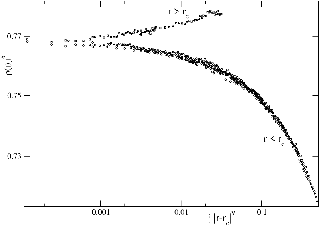
We compare these measurements with the established values of the DP exponents in table 1. We observe good agreement with the DP values that apply in one spatial dimension (1D) as long as we identify the exponent with the DP temporal correlation exponent , as opposed to the distinct, and independent, spatial exponent : we discuss this point in more detail shortly. For future reference, we have also included the exponents obtained within a mean-field approximation in table 1. For an in-depth study of DP exponents and scaling we refer the reader to [2]. Here, we focus more on the dynamic behaviour of the DACP and the behaviour of the active front as it moves out from the left boundary.
4.2 Advection dynamics: the shearing of DACP into DP
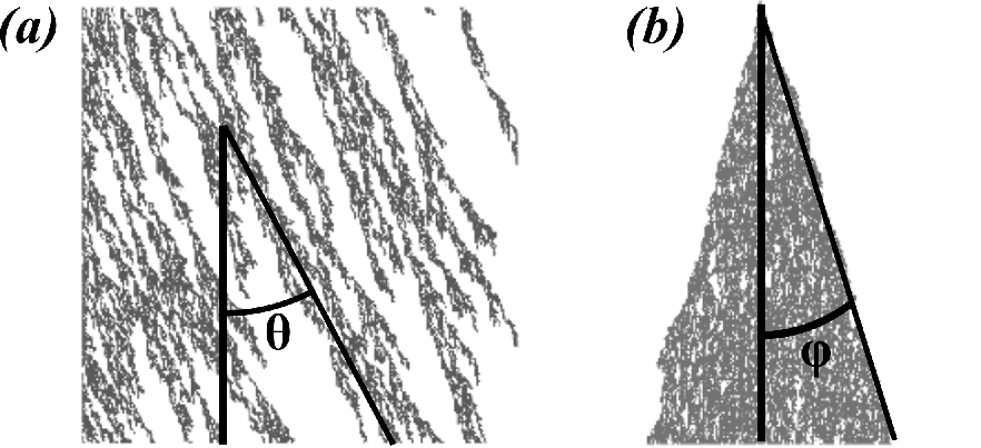
The easiest way to understand the effect of asymmetry (or advection) in the contact process is to directly compare a space-time plot of the DACP dynamics with its contact process counterpart and its description in terms of DP scaling exponents—see Fig. 6. From these plots we identify two characteristic angles. In the DACP, Fig. 6a, the activity emanates from the wall with an axis that is an angle to the vertical. This axis corresponds to the time direction in the basic contact process, Fig. 6b. The leading edge of the activity emerges at an angle to the DP time axis. We thus picture the DACP as a spatial shearing of DP by the shear element . One consequence of this shearing is that the spatial correlation length measured in the steady-state density profile of the DACP is a linear combination of the temporal and spatial correlations lengths in DP. Such that and , with primed variables pertaining to the DACP. Hence, we expect the DACP correlation length to diverge with the faster-growing DP correlation length as , and therefore that should be identified with the larger of the DP exponents (i.e., , as above).
We now turn to the dynamics. Above the critical point in DP, an activity wave travels at a velocity . If, near criticality, there is a single characteristic length and time scale, this velocity must be given by their ratio. That is
| (1) |
Since , this velocity vanishes as from above. Below criticality, activity does not spread out indefinitely, and so the wave velocity is zero when . Thus, the wave velocity is continuous across the transition in the absence of advection.
We obtain the supercritical wave velocity for the DACP, , by applying the shear . That is,
| (2) |
where we have introduced the advection . (There may be subleading corrections coming from corrections to scaling in the relation (1).) The actual value of is a nontrivial emergent property of the stochastic DACP dynamics. However, a key point is that it can take a nonzero value in the subcritical regime which yields the intrinsic velocity : activity still propagates at rate from the active boundary, despite the fact that it dies out after some finite time. Thus, the apparent (i.e. the observed) wave velocity, measured far from the origin, may jump discontinuously from zero to some nonzero value at the critical point. This is in contrast to the DP wave velocity which goes to zero at criticality, as shown above. The leading-order behaviour of the supercritical wave velocity in the DACP is then where . We remark that this expression provides a means to measure the smaller correlation length exponent, , which cannot be accessed from the steady-state density profile alone.
5 Mean-field theory
Having proposed a mechanism for the discontinuous velocity transition observed in section 3, we now demonstrate explicitly that it is at work within the mean-field formulation of the DACP dynamics.
We know that for a DP model, such as the contact process, the continuous-space mean-field description is given by a Fisher-KPP equation. The Fisher-KPP equation was first introduced in [21, 22, 23], see [11] for a review. We begin with the general form of the Fisher-KPP equation supplemented with an advection term to take into account the boundary drive present in the DACP:
| (3) |
At this stage and are phenomenological parameters. We will match these up with the parameters of the microscopic model in section 6.1 below. Meanwhile we note that we expect and to be smooth functions of the microscopic advection coefficient and that .
We first establish the two distinct stationary regimes which are determined by the sign of . If we set in (3) we find the stationary density is given by
| (4) |
The solution takes the following forms for large .
- For (subcritical case)
-
: a density profile which decays exponentially to zero and has the form for large ,
- For (supercritical case)
-
: a density profile which decays exponentially to a non-zero value and has the form for large , with .
In both cases the decay constant may be written as
| (5) |
For small , . Thus the characteristic lengthscale diverges as at criticality. Following the arguments of section 4, is expected to diverge with the DP exponent . From table 1, we see indeed that in the mean field.
Based on the envelope observed in the simulation of the stochastic system (see section 3) we assume that the full time-dependent density can be described by where is the stationary solution to (4). Equation (3) then becomes
| (6) |
Dividing through by and using the definition of , (4), to eliminate we obtain a modified Fisher-KPP equation for the wave that sits inside the envelope:
| (7) |
In this equation, the advective velocity of the modified wave, , is given by
| (8) |
Note that this advective velocity, , is generally increased over the bare quantity as a consequence of the envelope. The coefficient, of the non linear growth term is generally dependent, but in the supercritical phase it decreases to a constant value for large thus recovering the Fisher-KPP equation far from the boundary. On the other hand, in the subcritical regime the non-linear term decreases to zero far from the boundary.
First we consider the supercritical phase. Far from the boundary (7) becomes, using and
| (9) |
which is the usual Fisher wave equation with advective coefficient . Following the usual approach (see e.g. [11]), one assumes a travelling wave form and linearises for large where is small. The solution is of the form with
| (10) |
Since we require . We now assume (as for the normal Fisher wave starting from an initial sharp front) that . Thus
| (11) |
Of course (11) could simply be obtained by adding the advective velocity to the usual Fisher wave velocity in the absence of advection, .
In the subcritical phase, the modified wave described by (7) has a velocity given by a distinct expression. Here, for large , (7) becomes
| (12) |
where
| (13) |
Note that the advective velocity of the attenuated wave is increased over the value .
The spatial dependence of the coefficient of the non-linear term makes the analysis of equation (12) non-trivial. Here we content ourselves with a heuristic picture. Initially the presence of the nonlinear term will mean that a nonlinear travelling wave emanates from the boundary. However as the front moves away from the boundary the nonlinear term becomes less important and we expect the front to broaden and the velocity to decrease. Finally as the front of the wave moves further away and the equation for reduces to a diffusion equation with advection
| (14) |
The wavefront thus broadens diffusively over time. Therefore, at late times, the modified density profile will be approximately that given by a diffusion equation. This diffusive front moves with velocity
| (15) |
and the profile itself takes the form
| (16) |
Thus the width of the front is ultimately .
To summarise, the analysis of the phenomenological Fisher-KPP equation (3) shows that there are two possible regimes, according to the sign of . When is negative, the density decays to zero as it moves away from the origin; when positive, it propagates away from the origin with a constant bulk density at a constant velocity. The dynamics can be couched in terms of a modified wave, , travelling within the envelope of the steady-state density profile, . This wave is governed by the modified Fisher-KPP equation, (7), and has a velocity in these two states of and . Note that is continuous at the transition although its derivative is not.
In the subcritical regime, this velocity coincides with the advective velocity introduced in section 4 in terms of the angle of shear from DP to the DACP. As noted previously, one effect of the envelope is to force the apparent velocity (i.e., that observed in simulations) to decay to zero: activity can probe only a finite distance from the origin as time . Above the critical point, the observed velocity is and so, across the transition, this observed velocity exhibits a discontinuity. We note from the form of , the velocity grows from its critical value as where . This value of agrees with the prediction from the mean-field theory for DP (see table 1).
6 Modified travelling wave in the stochastic DACP
We now revisit the simulations of the DACP in the light of what we have learnt from the mean-field theory. We first express the phenomenological parameters appearing in the Fisher-KPP equation, (3), in terms of the stochastic activation rate . We then examine more closely the numerical evidence for the picture of an modified wave travelling within the stationary density profile, and in particular, the prediction for the growth of the wave velocity just above criticality, i.e., where given by the appropriate DP exponents.
6.1 Identification of the mean-field phenomenological parameters
We first revisit the mean-field theory of Section 5 and compare to the microscopic DACP dynamics. One may make and make a heuristic identification of the phenomenological parameters in (3) by considering first of all an exact equation for the rate of change of density at site in the DACP. This reads
| (17) |
where the first term comes from site activating site at rate if the former is active and the latter inactive, and the second term from the decay of site at unit rate when it is active. The mean-field approximation is to write , where .
| (18) | ||||
The steady state solution of this spatially discrete equation is provided in the appendix.
Here we move over to continuous space and expanding to second order spatial derivatives, we find, , , and , where . This suggests a density dependence in and : however, as we now explain, this is not expected to affect the wavefront behaviour.
In the subcritical regime the density profile tends to zero far from the boundary therefore and . Thus
| (19) |
In the supercritical regime, on the other hand, will tend to zero at the tip of the wavefront but be nonzero behind the Fisher wavefront. Thus at the tip and the supercritical Fisher wave velocity becomes
| (20) |
Therefore the derivative of the modified wave velocity is discontinuous at the phase transition. It is also interesting to note that with our identification of and , behind the wavefront in the supercritical regime we have and the effective advection is fixed at the critical value.
6.2 Stochastic modified wave dynamics
Returning now to the stochastic simulations of the DACP, we investigate first the picture of a modified wave travelling within a density envelope. In Fig. 4b, the density profile in the subcritical phase is shown at different time points along with an envelope of the form , with the fitting parameters all positive. As we get closer to criticality decreases, indicating an approach to the scaling form .
To obtain the modified wave , we divide the numerical density profiles by this envelope equation. The result of this procedure is shown in Fig. 7a, which clearly shows a wave with constant bulk density invading an empty lattice. The constancy of the wave velocity can be checked by dividing the coordinate by time (Fig. 7b). We do not, however, see strong evidence for the diffusive broadening of the wavefront predicted by (14). This could be because this equation applies only where the stationary density is small, a region that is a hard to access numerically.


A key component of the scaling picture (section 4), seen explicitly within the mean-field dynamics (section 5), is the continuity of the intrinsic wave velocity across the transition. After unfolding the envelope (as in Fig. 7) one can obtain this velocity over a range of activation rates . In Fig. 8, this velocity is compared with the apparent velocity before unfolding the velocity (i.e., the data of Fig. 3). The two velocities are clearly distinct in the subcritical regime (). Since the envelope decays exponentially in the subcritical phase, it is difficult to probe the late-time travelling-wave dynamics, and so the error bars on the modified wave velocity are necessarily large. However, the data suggest that the intrinsic velocity changes more slowly just below the critical point than above, in qualitative agreement with the mean-field predictions of equations (19),(20).

Finally, we attempt to access the exponent by fitting the observed wave velocity in the supercritical regime to the form suggested by the scaling picture of section 4 and confirmed within the mean-field regime by travelling wave analysis of section 5. It turns out that an estimate of is rather sensitive to the values of and used in a straight-line fit to plotted as a function of . Taking , we find the best fit (as quantified by the sum of square residuals) when . The corresponding plot is shown in Fig. 9 along with a line of gradient , which is the appropriate choice for DP in one dimension. We see that the simulation data have a gradient that is consistently higher than the predicted value. It may be that corrections to the leading-order behaviour remain significant in the region we have been able to access numerically. We remark that reasonable straight lines are obtained for values of in the range to , yielding estimates of between and suggesting that the numerical data are consistent with our scaling prediction for .

7 Conclusion
In this work we have studied a variation of the contact process which includes an active boundary which drives the system and advection away from that boundary. As expected the system exhibits a phase transition from a state with activity localised near the boundary to a state where a wave of activity emanates away from the boundary. We identify the DP critical exponents and by considering the behaviour of the density far from the boundary and the spatial decay length over which the density decays to that value. On the other hand, the velocity of the activity wave emanating from the boundary exhibits some perhaps unexpected behaviour: in the subcritical phase the apparent velocity is zero whereas in the supercritical phase the velocity jumps discontinuously to a non-zero value. We have explained this phenomenon by studying a mean field theory in which we show that an intrinsic velocity for a wave emanating from the boundary and described by (7), exists both below and above the transition. However in the subcritical regime the spatially decaying envelope for this wave means that the apparent velocity observed in the simulations is zero. This picture appears to hold well in simulations of the stochastic system
The study raises several interesting questions. At the mean field level it would be interesting to put our analysis of the modified Fisher equation (3), in particular the subcritical case, on a more rigorous footing. A study of the possible crossover in the solution of (3) from a nonlinear wave to a diffusive wave would be illuminating.
The noisy version of the Fisher-KPP equation is known to describe contact processes [24]. It would of course be of great interest to further understand travelling wave solutions of the noisy version of the Fisher-KPP equation, in particular the velocity and width of the front.
Appendix A Appendix: Solution of spatially discretized mean field equation
The mean-field equation (18) governing the density in the DACP process is
| (21) | ||||
The steady-state solution () is
| (22) |
which yields the large behaviour
| (23) | |||||
| (24) | |||||
| (25) |
Thus this mean field theory is consistent with the profiles decaying a decay length which diverges as and the order parameter emerging as where with . Also at criticality we have a power law decay of the profile with exponent . All these exponents are consistent with the mean field DP exponents given in Table 1.
References
- [1] T.E. Harris. Contact interactions on a lattice. Ann. Probab., 2:969–988, 1974.
- [2] H. Hinrichsen. Non-equilibrium critical phenomena and phase transitions into absorbing states. Adv. Phys., 49(7):815–958, 2000.
- [3] K.A. Takeuchi, M. Kuroda, H. Chaté, and M. Sano. Experimental realization of directed percolation criticality in turbulent liquid crystals. Phys. Rev. E, 80(5):051116, 2009.
- [4] C. Barrett-Freeman, M.R. Evans, D. Marenduzzo, and W.C.K. Poon. Nonequilibrium phase transition in the sedimentation of reproducing particles. Phys. Rev. Lett., 101(10):100602, 2008.
- [5] H.K. Janssen. On the nonequilibrium phase transition in reaction-diffusion systems with an absorbing stationary state. Z. Phys. B, 42(2):151–154, 1981.
- [6] P. Grassberger. On phase transitions in Schlögl’s second model. Z. Phys. B, 47(4):365–374, 1982.
- [7] C-C. Chen, H. Park, and M. den Nijs. Active width at a slanted active boundary in directed percolation. Phys. Rev. E, 60(3):2496–2500, 1999.
- [8] P. Fröjdh, M. Howard, and K.B. Lauritsen. Directed percolation and other systems with absorbing states: Impact of boundaries. Int. J. Mod. Phys. B, 15(12):1761–1798, 2001.
- [9] R.A. Blythe. Nonequilibrium phase transitions and dynamical scaling regimes. PhD thesis, University of Edinburgh, 2001.
- [10] M. Henkel, H. Hinrichsen, and S. Lubeck. Non-Equilibrium Phase Transitions: Absorbing Phase Transitions. Springer, 2008.
- [11] W. van Saarloos. Front propagation into unstable states. Phys. Rep., 386(2-6):29–222, 2003.
- [12] R.H. Schonmann. The asymmetric contact process. J. Stat. Phys., 44(3):505–534, 1986.
- [13] T. Sweet. The asymmetric contact process at its second critical value. J. Stat. Phys., 86(3):749–764, 1997.
- [14] R. Schinazi. The asymmetric contact process on a finite set. J. Stat. Phys., 74(5):1005–1016, 1994.
- [15] B. Derrida and D. Simon. The survival probability of a branching random walk in presence of an absorbing wall. Europhys. Lett., 78(6):60006, 2007.
- [16] D. Simon and B. Derrida. Quasi-stationary regime of a branching random walk in presence of an absorbing wall. J. Stat. Phys., 131(2):203–233, 2008.
- [17] C. Barrett-Freeman, M.R. Evans, D. Marenduzzo, and J. Tailleur. The role of noise and advection in absorbing state phase transitions. Europhys. Lett., 90(1):16003, 2010.
- [18] A.Y. Tretyakov, N. Inui, and N. Konno. Phase transition for the one-sided contact process. J. Phys. Soc. Jap., 66(12):3764–3769, 1997.
- [19] R.A. Blythe and M.R. Evans. Slow crossover to kardar-parisi-zhang scaling. Phys. Rev. E, 64(5):051101, 2001.
- [20] I. Jensen. Low-density series expansions for directed percolation: I. a new efficient algorithm with applications to the square lattice. J. Phys. A: Math. Gen., 32(28):5233–49, 1999.
- [21] R.A. Fisher. The wave of advance of advantageous genes. Ann. Eugen., 7:353–369, 1937.
- [22] A. Kolmogorov, I. Petrovskii, and N. Piskunov. Étude de l’équation de la diffusion avec croissance de la quantite de matière et son application à un problème biologique. Bull. Univ. État Moscou, A 1:1–25, 1937.
- [23] R. Luther. Räumliche fortpflanzung chemischer reaktionen. Z. Elektrochemie, 12(32):596–600, 1906.
- [24] C. Müller and R. Tribe. Stochastic pde’s arising from the long-range contact and long-range voter processes. Probab. Theory Relat. Fields, 102(4):519–545, 1995.