Rubber friction and tire dynamics

1. Introduction

Rubber friction is a topic of huge practical importance, e.g., for tires, rubber seals, conveyor belts and syringes[1, 2, 3, 4, 5, 6, 16, 7, 8, 9, 10, 11, 12, 13, 14, 15, 17]. In most theoretical studies rubber friction is described using very simple phenomenological models, e.g., the Coulombs friction law with a friction coefficient which may depend on the local sliding velocity. However, as we have shown earlier[6], rubber friction depends on the history of the sliding motion (memory effects), which we have found to be crucial for an accurate description of rubber friction. For rubber sliding on a hard rough substrate, the history dependence of the friction is mainly due to frictional heating in the rubber-substrate contact regions. Many experimental observations, such as an apparent dependence of the rubber friction on the normal stress, can be attributed to the influence of frictional heating on the rubber friction.

A huge number of papers have been published related to tire dynamics, in particular in the context of Anti-Blocking System (ABS) braking models. The “heart” in tire dynamics is the road-rubber tire friction. Thus, unless this friction is accurately described, no tire model, independent of how detailed the description of the tire body may be, will provide an accurate picture of tire dynamics. However, most treatments account for the road-tire friction in a very approximate way. Thus, many “advanced” finite element studies for tire dynamics account for the friction only via a static and a kinetic rubber friction coefficients. In other studies the dynamics of the the whole tire is described using interpolation formulas, e.g., the “Magic Formula”[4], but this approach require a very large set of measured tire properties (which are expensive and time-consuming to obtain), and cannot describe the influence of history (or memory) effects on tire dynamics.

In this paper we first propose a very simple rubber friction law (with memory effects) which gives nearly identical results to the full model developed in Ref. [6]. We also develop a 2D-tire model which combines the rubber-road friction theory (which accounts for the flash temperature) with a simple two-dimensional (2D) description of the tire body. We believe that the most important aspect of the tire body is its distributed mass and elasticity, and this is fully accounted for in our model. One advantage of the 2D-model over a full 3D-model is that one can easily impose any foot-print pressure distribution one like (e.g., measured pressure distributions), while in a 3D-model the pressure distribution is fixed by the model itself. This allow a detailed study on how sensitive the tire dynamics depends on the nature of the foot print pressure distribution. The tire model is illustrated by calculating $\mu$-slip curves, and with simulations of ABS braking using two different control algorithms.

2. Rubber friction

Rubber friction depends on the history of the sliding motion. This is mainly due to the flash temperature: the temperature in the rubber-road asperity contact regions at time $t$ depends on the sliding history for all earlier times $t^{\prime}<t$. This memory effect is crucial for an accurate description of rubber friction. We illustrate this effect in Fig. 1 for a rubber tread block sliding on an asphalt road surface. We show the (calculated) kinetic friction coefficient for stationary sliding without (blue curve) and including the flash temperature (red curve) as a function of the velocity $v$ of the bottom surface of the rubber block. The black curves shows the effective friction during non-stationary sliding experienced by a rubber tread block during braking at various slips (slip values from 0.005 to 0.09). Note that because some finite sliding distance is necessary in order to fully develop the flash temperature, the friction acting on the tread block initially follows the blue curve corresponding to “cold-rubber” (i.e., negligible flash temperature). Thus, it is not possible to accurately describe rubber friction with just a static and a kinetic friction coefficients (as is often done even in advanced tire dynamics computer simulation codes) or even with a function $\mu(v)$ which depends on the instantaneous sliding velocity $v(t)$. Instead, the friction depends on $v(t^{\prime})$ for all times $t^{\prime}\leq t$.

As a background to what follows, we first review the rubber friction theory (see [6, 5] for details). It is assumed that all energy dissipation arises from the viscoelastic deformations of the rubber surface by the road asperities. An asperity contact region with the diameter $d$ gives rise to time dependent (pulsating) deformations of the rubber which is characterized by the frequency $\omega=v/d$, where $v$ is the sliding velocity. The viscoelastic deformation (and most of the energy dissipation) extend into the rubber by the typical distance $d$. So most of the energy dissipation occur in a volume element of order $d^{3}$. In order to have a large asperity-induced contribution to the friction the frequency $\omega$ should be close to the maximum of the ${\rm tan}\delta={\rm Im}E(\omega)/{\rm Re}E(\omega)$ curve. Here $E(\omega)$ is the viscoelastic modulus of the rubber. In reality there will be a wide distribution of asperity contact sizes, so there will be a wide range of perturbing frequencies, say from $\omega_{0}$ to $\omega_{1}$, see Fig. 2. A large friction requires that ${\rm tan}\delta$ is as large as possible for all these perturbing frequencies.

The temperature dependence of the viscoelastic modulus of rubber-like materials is usually very strong, and an increase in the temperature by $10\ ^{\circ}{\rm C}$ may shift the ${\rm tan}\delta$ curve to higher frequencies by one frequency decade. This will usually reduce the rubber friction, see Fig. 2.

Real surfaces have a wide distribution of asperity sizes. The best picture of a rough surface is to think about it as big asperities on top of which occur smaller asperities on top of which occur even smaller asperities … . This is illustrated in Fig. 3 for a case where roughness occur on two length scales. To get the total energy dissipation during sliding on a real surface one need to sum up the contribution from asperity induced deformation of the rubber on all (relevant) length scales. It is important to note that all length scales are a priory equally important[5].

Temperature has a crucial influence on rubber friction. The viscoelastic energy dissipation, which is the origin of the rubber friction in my model, result in local heating of the rubber in exactly the region where the energy dissipation occur. This result in a temperature increase, which becomes larger as we observe smaller and smaller asperity contact regions. This local (in time and space) temperature increase, resulting from the local viscoelastic energy dissipation, is referred to as the flash temperature. The flash temperature has an extremely important influence on the rubber friction. This is illustrate in Fig. 1, where we show the (calculated) steady state kinetic friction coefficient when a block of tread rubber is sliding on an asphalt road surface. The upper curve is the result without accounting for the flash temperature, i.e., the temperature is assumed to be equal to the background temperature $T_{0}$ everywhere. The lower curve is the result including the flash temperature. Note that for sliding velocities $v>0.001\ {\rm m/s}$ the flash temperature result in a lowering of the sliding friction. For velocities $v<0.001\ {\rm m/s}$ the produced heat has enough time to diffuse away from the asperity contact regions, and the flash temperature effect is negligible.

In the rubber friction theory the concept of the macroasperity contact region is of crucial importance. Let us study the footprint contact region between a tire and a road surface at different magnification $\zeta$. At low magnification the road surface appears smooth and the contact between the tire and the road appears to be complete within the footprint area as in Fig. 4(a). However, when we increase the magnification $\zeta$ we start to observe non-contact regions as in Fig. 4(b). At high enough magnification we observe isolated contact regions as in Fig. 4(c), which, when the magnification increases even further, break up into even smaller contact regions as in Fig. 4(d). We denote the contact regions observed in Fig. 4(c) as the macroasperity contact regions (with the average diameter $D$) (the exact definition is given in Ref. [6, 18]). If the nominal pressure in the tire-road contact region is small the macroasperity contact regions will be well separated, but the separation between the microasperity contact regions within the macroasperity contact regions is in general very small. When calculating the flash temperature effect we have therefore smeared out the heat produced by the microasperity contact regions uniformly within the macroasperity contact regions. Typically for road surfaces $D\approx 0.1-1\ {\rm cm}$, and the fraction of the tread block surface occupied by the macroasperity contact regions are typically between $10\%$ and $30\%$.

In the friction theory developed in Ref. [6] only the surface roughness with wave vectors $q<q_{1}$ are assumed to contribute to the friction. For clean road surfaces we determine the cut-off wavevector $q_{1}$ by a yield condition: We assume that the local stress and temperature in the asperity contact regions on the length scale $1/q_{1}$ are so high that the rubber bonds break resulting in a thin modified (dead) layer of rubber at the surface region of thickness $\approx 1/q_{1}$. From this follows the following observations:

(a) The rubber friction on clean road surfaces after run-in is rather insensitive to the road surface. This has been observed in several series of experimental studies (not shown), and is in accordance with the present theory. This can be understood as follows. The cut-off $q_{1}$ on surfaces with smoother, less sharp roughness or surfaces where the roughness occur at shorter length scales will be larger (i.e. the cut-off wavelength $\lambda_{1}=2\pi/q_{1}$ smaller) than for road surfaces with larger roughness in such a way as the stress and temperature increase in the asperity contact regions which can be observed at the resolution $\lambda_{1}$ (or magnification $\zeta=q_{1}/q_{0}$) are roughly the same on all surfaces. This implies that a larger range of roughness will contribute to the rubber friction on “smoother” surfaces as compared to more rough surfaces. As a consequence, the friction (after run-in) may vary very little between different (clean) road surfaces.

(b) On contaminated road surfaces, the cut-off $q_{1}$ may be determined by the nature of the contamination. In this case, if the cut-off is fixed (e.g., determined by, say, the size of contamination particles) one may expect much larger variation in the friction coefficient between different road surfaces, and also a larger variation between tired with different types of tread rubber.

3. Phenomenological rubber friction law

In tire applications, for slip of order $5-10\%$ and typical footprint length of order $10\ {\rm cm}$, the slip distance of a tread rubber block in the footprint will be of order $1\ {\rm cm}$, which typically is of order the diameters $D$ of the macro asperity contact regions. As discussed above, as long as the slip distance $s(t)$ is small compared to $D$ one follow the cold rubber branch of the steady state relation $\mu(v)$ so that $\mu(t)\approx\mu_{\rm cold}(v(t))$ for the slip distance $s(t)<<D$. When the tread block moves towards the end of the footprint the slip distance $s(t)$ may be of order of (or larger than) $D$, and the friction will follow the hot branch of the $\mu(v)$ relation i.e., $\mu(t)\approx\mu_{\rm hot}(v(t))$ for $s(t)>D$. We have found that the following (history dependent) friction law gives nearly the same result as the full theory presented in Ref. [6]:

where $v(t)$ is the instantaneous sliding velocity and $s(t)$ the sliding distance, and $s_{0}\approx 0.2D$. We will refer to (1) as the cold-hot friction law. The length $D$ depends on the rubber compound and the road surface but is typically in the range $D\approx 0.1-1\ {\rm cm}$. Using the full friction theory one can easily calculate the functions $\mu_{\rm cold}(v(t),T_{0})$ and $\mu_{\rm hot}(v(t),T_{0})$ and the length $D$.

To demonstrate the accuracy of the cold-hot rubber friction law (1), let us study the dynamics of one tread block as it pass through the tire-road footprint. In Fig. 5 we show the the frictional shear stress acting on a tread block as a function of time for many slip values: $0.005$, $0.0075$, $0.01$, $0.03$, $0.05$, $0.07$, $0.09$, $0.12$, $0.15$ and $0.25$. Note that the cold-hot friction law (1) (red curves) gives nearly the same result as for the full friction model (green curves). In Fig. 6 we show the $\mu$-slip curve. Again the cold-hot friction law (1) (red curve) gives nearly the same result as the full friction model (green curve).

4. Tire dynamics

All the calculations presented in this section have been obtained using the 2D tire model described below, with the tire body optimized using experimental data for a passenger car tire. The viscoelastic springs associated with this tire body are kept fixed in all the calculations. Thus the model calculations does not take into account the changes in the tire body viscoelastic properties due to variations in the tire (background) temperature, or variations in the tire inflation pressure (which affect the tension in the tire walls). In principle both effects can be relatively simply accounted for in the model, but have not been included so far. All the calculations presented below are obtained using the measured viscoelastic modulus of a passenger car tire tread compound, and for the Estoril racer track.

We use a 2D-description of the tire body as indicated in Fig. 7. We introduce a coordinate system with the $y$-axis in the transverse direction and the $x$-axis along the longitudinal (rolling) direction. We consider the tire-road system in a reference frame where the road is stationary. The car velocity $v_{\rm c}$, the rolling velocity $v_{\rm R}$ and the cornering angle $\theta$ determines the transverse $v_{y}$ and longitudinal $v_{x}$ slip velocities:

The longitudinal slip is defined by

When the cornering angle $\theta=0$ this equation reduces to

Note that $v_{x}$ and $v_{y}$ are also the velocities of the tire rim, and that the footprint moves (in the rolling direction) with the velocity $v_{\rm c}{\rm cos}\theta$ relative to the road, and with the rolling velocity $v_{\rm c}{\rm cos}\theta-v_{x}=v_{\rm R}$ relative to the rim.

We describe the tire body as a set of mass points connected with viscoelastic springs (elasticity $k$ and viscous damping $\gamma$). The springs have both elongation and bending elasticity, denoted by $k$ and $k^{\prime}$, respectively, and the corresponding viscous damping coefficients $\gamma$ and $\gamma^{\prime}$. We assume $N_{x}$ and $N_{y}$ tire body blocks along the $x$- and $y$-directions and let ${\bf x}_{ij}=(x_{ij},y_{ij})$ denote the displacement vector of tire body block $(i,j)$ ($i=1,...,N_{x}$, $j=1,...,N_{y}$). Since the tire is a torus shaped object we must assume periodic boundary conditions in the $x$-direction so that $x_{N_{x}+1,j}=x_{1,j}$ and $y_{N_{x}+1,j}=y_{1,j}$.

For stationary tire motion we have the following boundary conditions. For $i=0,...,N_{x}+1$:

For $j=1,...,N_{y}$:

If the mass of tire body element $(i,j)$ is denoted by $m_{j}$, we get for $i=1,...,N_{x}$, $j=1,...,N_{y}$:

In the equations above, $F_{xij}$ and $F_{yij}$ are the force components (in the $x$- and $y$-directions, respectively) acting on the tire body block $(i,j)$ from the tread block $(i,j)$. Thus, ${\bf F}_{ij}=(F_{xij},F_{yij})$ is nonzero only when $(i,j)$ is in the tire tread area. The tire body viscoelastic spring parameters $(k,\gamma)$ and $(k^{\prime},\gamma^{\prime})$ in the tread area and in the side wall area (8 parameters) have been optimized in order to reproduce a number of measured tire properties (e.g., the longitudinal and transverse tire stiffness values for three tire loads, and the frequency and damping of the lowest longitudinal and transverse tire vibrational modes). The optimization has been performed using the amoeba method of multidimensional minimization[19].

4.1 Dependence of the $\mu$-slip curve on the shape of the tire-road footprint

Here we will study how the tire dynamics depends on the shape of the tire-road footprint. We consider the rectangular, elliptic and trapezoid footprints shown Fig. 8. We assume first that the pressure in the footprint is uniform and equal to $p=0.1\ {\rm MPa}$, and that the tire load is equal to $2000\ {\rm N}$ in all cases. Thus all the foot prints have the same area.

In Fig. 9 we show the $\mu$-slip curves for the three footprints shown in Fig. 8, and in Fig. 10 we show the corresponding $\mu$-slip angle curves. It is remarkable how insensitive the results are to the shape of the footprint. Thus we may state that $\mu$-slip curves, and hence tire dynamics, depends very weakly on the shape of the tire-road footprint, assuming everything else the same.

In Fig. 11 we show the the self-aligning moment for the trapezoid footprint profile in Fig. 8, as a function of the longitudinal slip (for zero cornering angle). Note that for the rectangular and elliptic footprint the self aligning moment vanish (not shown). This is expected because of the mirror symmetry of the footprint in the $x$-axis through the center of the footprint. However, the trapezoid footprint does not exhibit this symmetry (see Fig. 8), and the self aligning moment is non-vanishing in this case.

In Fig. 12 we show the self-aligning moment for the three footprints shown in Fig. 8, as a function of the cornering angle (for zero longitudinal slip). In this case the self aligning moment is non-vanishing in all cases. It is remarkable, however, how insensitive the results are to the shape of the footprint.

For small $\theta$ the self aligning moment is positive. This is due to the gradual (nearly linear) build up of the transverse stress from the inlet of the footprint to the exit. Thus the center of mass of the frictional stress distribution is located closer to the exit of the footprint giving a positive self aligning moment. For large $\theta$ the self aligning moment is negative. In the present model this is due to the flash temperature effect: when a tread block enter the footprint the rubber is “cold”, and initially the rubber friction is high. After a short slip distance the full flash temperature is built up and the rubber friction is smaller. This will result in a frictional stress distribution which is larger close to the inlet. This in turn result in a negative self aligning moment.

In the study above we have assumed a constant pressure in the footprints. In reality, the pressure will be slightly larger at the inlet than at the exit of contact with the road (this is the case also during pure rolling and is related to the rolling resistance). This asymmetry will give an additional (negative) contribution to self aligning moment for large slip.

In Fig. 13 we show the $\mu$-slip angle curves for the three footprints shown in Fig. 8, and for the longitudinal slip $s=0$ and $s=0.03$. Note, in accordance with experimental observations, for the combined slip $\mu_{y}(\theta)$ is smaller than for the case when the longitudinal slip vanish. Again there is very little influence on the shape of the footprint. However, the self aligning moment will now depend strongly on the shape of the footprint. This is shown in Fig. 14 for the case $s=0.03$. Note that for the trapezoid footprint the self aligning moment is much larger than for the elliptic and rectangular footprints. This is due to the contribution from the longitudinal stress component which gives rise to a net longitudinal force centered to the right of the mid-line of the tire.

Fig. 15 shows the $\mu$-slip angle curves (a), and the self aligning moment (b) for the elliptic footprint for the tire load $F_{\rm N}=3000$, $5000$ and $7000\ {\rm N}$, and the footprint pressure $p=0.3\ {\rm MPa}$. Note that as the load increases the foot print becomes longer which result in a decrease in the maximum friction coefficient, which agree with experimental observations. This load-dependence is not due to an intrinsic pressure dependence of the rubber friction coefficient (which was kept constant in our calculation), but a kinetic effect related to the build up of the flash temperature in rubber road asperity contact regions during slip. To understand this in more detail, consider again Fig. 1.

The red and blue lines in Fig. 1 show the kinetic friction coefficient (stationary sliding) as a function of the logarithm of the sliding velocity. The upper line denoted “cold” is without the flash temperature while the lower line denoted “hot” is with the flash temperature. The black curves show the effective friction experienced by a tread block as it goes through the footprint. Results are shown for several slip values $0.005$, $0.0075$, $0.01$, $0.03$, $0.05$, $0.07$ and $0.09$. Note that the friction experienced by the tread block first follows the “cold” rubber branch, and then, when the block has slipped a distance of order the diameter $D$ of the macroasperity contact region, it follows the “hot” rubber branch. Based on this figure it is easy to understand why the maximum friction coefficient increases when the length of the footprint decreases: If $v_{\rm slip}$ is the (average) slip velocity of the tread block, then in order to fully build up the flash temperature the following condition must be satisfied: $v_{\rm slip}t_{\rm slip}\approx D$, where $D$ is the diameter of the macroasperity contact region. Since the time the rubber block stay in the footprint $t_{\rm slip}=L/v_{\rm R}$ (where $L$ is the length of the footprint and $v_{\rm R}$ the rolling velocity) we get $v_{\rm slip}\approx v_{\rm R}(D/L)$. Thus, when the length $L$ of the footprint decreases, the (average) slip velocity of the tread block in the footprint can increase without the slip distance exceeding the diameter $D$ of the macro asperity contact region. Thus at the slip corresponding to the maximum of the $\mu$-slip curve, for a short footprint, as compared to a longer footprint, the tread block will follow the “cold” rubber branch of the (steady state) $\mu$-slip curve to higher slip velocities before the flash temperature is fully developed, resulting in a higher (maximal) tire-road friction for a short footprint as compared to a longer footprint.

In Fig. 16 we show snapshot pictures of the tire body deformations for three cases, namely with the slip $s$ and the coornering angle $\theta$ given by $(s,\theta)=(0.05,0)$ (left), $(0.03,5^{\circ})$ (middle) and $(0,5^{\circ})$ (right). The open squares denote the position of rubber elements of the undeformed tire body, and the filled squares underneath denote the position of the same tire body elements of the deformed tire.

In Fig. 17 we show snapshot pictures of the tire body deformations for the rectangular, trapezoid and elliptic contact area with contact pressure $0.3\ {\rm MPa}$ and normal load $F_{\rm N}=7000\ {\rm N}$. In all cases the slip $s=0.05$ and the coornering angle $\theta=0$. Note how insensitive the deformation field is to the shape of the footprint. This is caused by the high stiffness of the tire body in the tread area.

4.2 Dependence of the $\mu$-slip curve on the size of the tire-road footprint

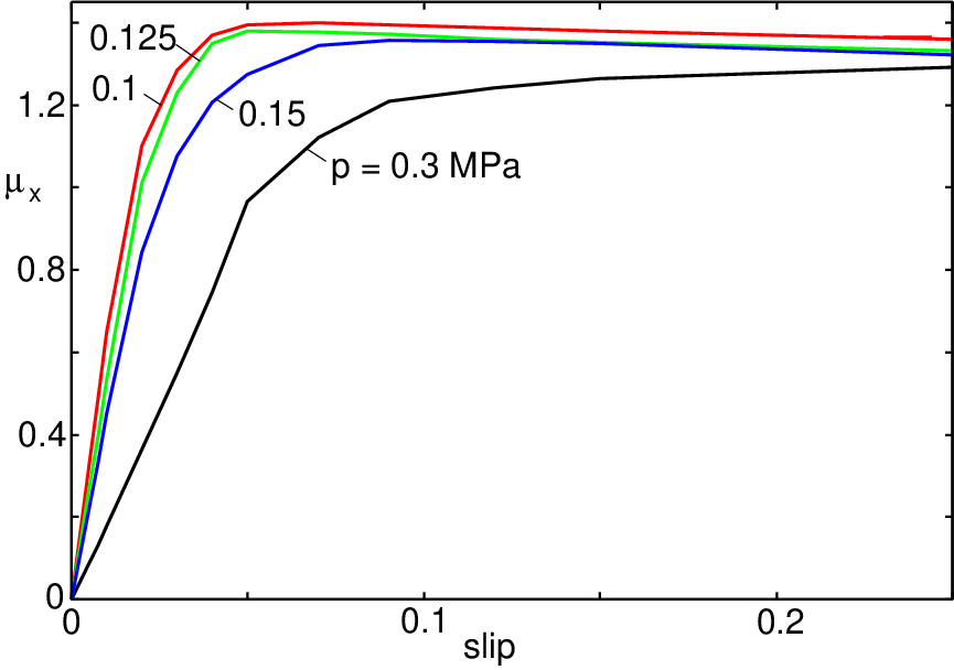
In Fig. 18 we show $\mu$-slip curves for the rectangular footprint for the contact pressures $p=0.1$, $0.125$, $0.15$ and $0.3\ {\rm MPa}$. The tire load is fixed at $F_{\rm N}=2000$ so the different contact pressures corresponding to the footprint length $L=10.2$, $8.1$, $6.8$ and $3.4\ {\rm cm}$, respectively. Note that increasing the tire footprint pressure decreases the length of the footprint, which decreases the tire longitudinal stiffness $C_{x}$ (determined by the initial slope of the $\mu_{x}(s)$-curves), and also the maximum of the $\mu$-slip curves. In practice the pressure in the tire-road footprint can be changed by changing the tire inflation pressure, but in this case one expect also a change in the tire body stiffness. In the tire model we use this effect is not included at present. Thus, at least for passenger car tires, when the inflation pressure increases the longitudinal tire stiffness $C_{x}$ usually first increases and then, at high enough inflation pressure, decreases. This is consistent with Fig. 18 which shows initially a very small change in the tire stiffness as the footprint pressure $p$ increases, so that for small (but not too small) $p$, the stiffening of the tire body may dominate over the contribution from the change in the footprint, so that initially $C_{x}$ increases with increasing $p$.

In Fig. 19 we show snap shot pictures of the tire body deformations for three cases, namely for the external load $F_{\rm N}=3000$, $5000$ and $7000\ {\rm N}$. In all cases the slip $s=0.05$ and the coornering angle $\theta=0$. The results are for the rectangular footprint with contact pressure $0.3\ {\rm MPa}$.

In Fig. 20 we show similar results as in Fig. 19 but now for the elliptic contact area with contact pressure $0.3\ {\rm MPa}$, and with the slip $s=0$ and the coornering angle $\theta=5^{\circ}$. The maximum tire body displacements are $1.20$, $1.81$ and $2.31\ {\rm cm}$ for the tire loads $F_{\rm N}=3000$, $5000$ and $7000\ {\rm N}$, respectively.

In Fig. 21 we show the maximum friction coefficient, $\mu_{\rm max}$, of the $\mu_{x}$-slip curve for the elliptic, rectangular and trapezoid footprints, as a function of the tire load. We show results for the contact pressures $p=0.1\ {\rm MPa}$ (upper three curves) and $0.3\ {\rm MPa}$ (lower three curves), but the tire body properties are assumed to be the same. Note that the effective friction depends on the (average) tire-road footprint pressure $p$. When $p$ increases, assuming unchanged size of the footprint, the friction decreases. This is one reason for why racer tires exhibit much larger friction than passenger car tires (the contact pressure in F1 tires is of order $0.1\ {\rm MPa}$ which is about 3 times lower than in passenger car tires). The increase in the friction as the tire-road contact pressure $p$ decreases is mainly due to a decrease in the pressure in the macro asperity contact regions as $p$ decreases: When the local pressure decreases the produced heating of the rubber decreases leading to a larger friction.

In Fig. 22 we show for the same systems the longitudinal tire stiffness $C_{x}$ associated with the $\mu_{x}$-slip curves. Finally, Fig. 23 gives the maximum longitudinal tire body displacement as a function of the tire load, for the same systems as in Fig. 21.

4.3 Dependence of the $\mu$-slip curve on the car velocity

Fig. 24 shows the the $\mu$-slip curves for the rectangular footprint ($20\ {\rm cm}\times 10.2\ {\rm cm}$) shown in Fig. 8, and for the car velocities $v_{\rm c}=10$, $30$ and $40\ {\rm m/s}$. We show results both for the tire load $F_{\rm N}=2000\ {\rm N}$ and $p=0.1\ {\rm MPa}$ (top three curves) and for $F_{\rm N}=6000\ {\rm N}$ and $p=0.3\ {\rm MPa}$ (lower three curves). Note that as the car velocity decreases the longitudinal tire stiffness $C_{x}$ decreases and the maximum of the $\mu$-slip curve increases. This is in accordance with experimental observations for passenger car tires (see, e.g., Fig. 8.65 in Ref. [3]). When the contact pressure and the load both increases, in such a way that the contact area stays constant, both the tire stiffness and the maximum of the $\mu$-slip curves decreases.

5. ABS braking simulations

The theory developed above may be extremely useful to design or optimize control algorithms for ABS braking. Here we will present results using the two simplest possible control algorithms. In both cases the braking torque is changed (increase or decrease) in steps of $\Delta M$ at time $t_{n}=n\Delta t$ $(n=1,2,...)$. The first algorithm (a) assumes that the slip $s^{*}$ where the friction is maximal is known (and constant in time). In this case the braking torque is increased if the slip $s(t_{n})$ at time $t_{n}$ is below $s^{*}$ and otherwise it is decreased, see Fig. 25. One problem here is that the slip $s^{*}$ depends on the car velocity which change during the braking process. However, in the present case $s^{*}\approx 0.057$ nearly independent of the car velocity for $10\ {\rm m/s}<v_{\rm c}<27\ {\rm m/s}$.

In the second control algorithm (b) we assume that $s^{*}$ is unknown. Nevertheless, by registering if the (longitudinal) friction $F_{x}(t)$ is increasing or decreasing with time we can find out if we are to the left or right of the maximum at $s=s^{*}$. That is, if

or if

then we must have $s(t_{n})>s^{*}$ and the braking torque at time $t_{n}$ is reduced, otherwise it is increased. Here $F_{x}(t_{n})$ is the longitudinal friction force and $s(t_{n})$ the slip at time $t_{n}=n\Delta t$ $(n=1,2,...)$.

We now present numerical results to illustrate the two ABS braking algorithm. Let $M$ be the mass-load on a wheel and $I$ the moment of inertia of the wheel without the tire. We assume for simplicity that the suspension is rigid and neglect mass-load transfer. The equations of motion for the center of mass coordinate $x(t)$ of the wheel, and for the angular rotation coordinate $\phi(t)$ are:

where $F_{\rm rim}$ is the force acting on the rim, $M_{\rm B}$ is the braking torque and $M_{\rm rim}$ the torque acting on the rim from the tire (for constant rolling velocity $F_{\rm rim}=F_{\rm f}$ is the tire-road friction force and $M_{\rm rim}=RF_{\rm f}$, where $R$ is the rolling radius, but during angular accelerations these relation no longer holds because of tire inertia effects) We have used $M=360\ {\rm kg}$ and $I=0.4\ {\rm kgm^{2}}$.

We assume first the control algorithm (a). We take $\Delta M=200\ {\rm Nm}$ and $\Delta t=0.03\ {\rm s}$, and we assume (see Fig. 25) $s^{*}\approx 0.05$. In Fig. 26 we show (a) the car velocity $v_{\rm c}$ and the rolling velocity $v_{\rm R}$, (b) the longitudinal slip and (c) the braking torque as a function of time. The time it takes ($t=1.775\ {\rm s}$) to reduce the car velocity from $v_{0}=27$ to $v_{1}=10\ {\rm m/s}$ correspond to a friction coefficient $\mu=(v_{0}-v_{1})/gt=0.976$ which is $\sim 13\%$ smaller than the friction at the maximum of the $\mu$-slip curve, which varies between $\mu_{\rm max}=1.14$ and $1.11$ as the car velocity changes from $27$ to $10\ {\rm m/s}$. The slope of the car-velocity line in Fig. 26(a) for $t>0.2\ {\rm s}$ correspond to the friction coefficient $1.02$, which is larger than the (average) friction calculated from the stopping time. The slightly smaller friction obtained from the stopping time reflect the (short) initial time interval necessary to build up the braking torque.

In Fig. 27 we show results for the ABS control algorithm (b). Note that it takes $t=1.949\ {\rm s}$ to reduce the car velocity from $v_{0}=27\ {\rm m/s}$ to $v_{1}=10\ {\rm m/s}$. This correspond to the effective friction coefficient $\mu=(v_{0}-v_{1})/gt=0.889$. The maximum in the $\mu$-slip curve (see Fig. 25) depends on the car velocity but is about $\mu_{\rm max}=1.14$ for $v_{\rm c}=27\ {\rm m/s}$ and about $1.11$ for $v_{\rm c}=10\ {\rm m/s}$ so the ABS braking control algorithm used above could still be improved. Note also that the wheel tend to lock about 3 or 4 times per second. This is in good agreement with ABS braking systems presently in use. However, since the speed of cars are usually not known during ABS braking, braking control algorithms used in most cars today determine the braking torque only from the wheel rotation acceleration. This is possible because, as shown in Fig. 27(a), as the wheel tend to lock, the rotational velocity very rapidly decreases, and it this point the ABS system decreases the braking torque.

Note that the (average) of the slip in Fig. 26(b) and 27(b) increases with increasing time or, equivalently, decreasing car velocity. This is mainly due to the fact that the time it takes for the wheel to lock, when the slip $s>s^{*}$, decreases as $v_{\rm c}$ decreases. Thus, during the time period $\Delta t$ between two changes in the brake torque the maximal slip (corresponding to the minimal rolling velocity) will increase as $v_{\rm c}$ decrease. This is easy to show mathematically. Since the car velocity changes slowly compared to the rolling velocity, from the definition $s=(v_{\rm c}-v_{\rm R})/v_{\rm c}$ we get

If we approximate the $\mu$-slip curve for $s>s^{*}$ with a strait line,

we get from (3)

or

where $A=(MgR\mu_{0}-M_{\rm B})(R/Iv_{\rm c})$ and $B=\Delta\mu(MgR^{2}/Iv_{\rm c})$. Since $A$ and $B$ can be considered as constant during the time interval between the changes in the braking torque, we get

where

It is easy to show that

where $M_{\rm B}^{*}=Mg(\mu_{0}-\Delta\mu s^{*})$ is the braking torque necessary in order to stay at the maximum in the $\mu$-slip curve. If $M_{\rm B}<M_{\rm B}^{*}$ and $s(0)>s^{*}$ we have $s(0)-A/B>0$ and during the time interval $\Delta t$ the slip will increase with $[s(0)-A/B]{\rm exp}(B\Delta t)$. Since $B\Delta t\sim 1/v_{\rm c}$ the maximum slip will increase exponentially (until the wheel block, corresponding to $s=1$) with the inverse of the car velocity. This behavior (i.e., the increase in the slip with decreasing car velocity) can be seen in Fig. 26(b) and is even stronger for the second ABS control algorithm [fig. 27(b)].

In Fig. 28 we show the $\mu$-slip curve during stationary slip (green curve) and the instantaneous effective friction coefficient $\mu_{\rm eff}(t)=F_{x}(t)/F_{\rm N}$ during braking (blue curve).

The blue and red curves in Fig. 29 show the car velocity using the ABS control algorithms (a) and (b). It is clear that the ABS control algorithm (a) is more effective than algorithm (b), but algorithm (a) assumes that $s^{*}$ is known and remains constant during the braking event.

The ABS braking control algorithms used today usually assumes that only the wheel rolling velocity $v_{\rm R}(t)$ is known. Basically, whenever a wheel tend to lock-up, which manifest itself in a large (negative) wheel angular acceleration, the braking torque is reduced. These ABS braking control algorithms (e.g., the Bosch algorithm) are rather complex and secret. The calculations presented above can be easily extended to such realistic ABS braking control algorithms and to more complex cases such as braking during load fluctuations (e.g., braking on uneven road surfaces) and switching between different road surfaces (by using different road surface power spectra’s during an ABS braking simulation).

6. Summary and conclusion

In this paper we have proposed a simple rubber friction law, which can be used, e.g., in models of tire (and vehicle) dynamics. The friction law gives nearly the same result as the full rubber friction theory of Ref. [6], but is much more convenient to use in numerical studies of, e.g., tire dynamics, as the friction force can be calculated much faster.

We have proposed a two-dimensional (2D) tire model which combines the rubber friction law with a simple mass-spring description of the tire body. The tire model is very flexible and can be used to calculate accurate $\mu$-slip (and the self-aligning torque) curves for braking and cornering or combined motion (e.g., braking during cornering). We have presented numerical results which illustrate the theory. Simulations of Anti-Blocking System (ABS) braking was performed using two simple control algorithms.

References

- [1] B.N.J. Persson, Sliding Friction: Physical Principles and Applications, 2nd edn (2000) (Heidelberg, Springer).
- [2] K.A. Grosch, Proc. R. Soc. London, Ser. A274, 21 (1963).
- [3] The Pneumatic Tire, edited by A.N. Gent and J.D. Walter, US Department of Transportation (2006).
- [4] H.B. Pacejka, Tyre and Vehicle Dynamics, 2nd edn (2006) (Amsterdam, Elsevier).
- [5] B.N.J. Persson, J. Chem. Phys. 115, 3840 (2001).
- [6] B.N.J. Persson, J. Phys.: Condensed Matter 18, 7789 (2006).
- [7] G. Heinrich, M. Klüppel and T.A. Vilgis, Comp. Theor. Polym. Sci. 10, 53 (2000).
- [8] G. Heinrich and M. Klüppel, Wear 265, 1052 (2008).
- [9] S. Westermann, F. Petry, R. Boes and G. Thielen, Kautsch. Gummi Kunstst. 57, 645 (2004).
- [10] B.N.J. Persson and A.I. Volokitin, Eur. Phys. J. E21, 69 (2006).
- [11] G. Carbone, B. Lorenz, B.N.J. Persson and A. Wohlers, Eur. Phys. J. E29, 275 (2009).
- [12] B.N.J. Persson, Surf. Sci. 401, 445 (1998).
- [13] A. Le Gal and M. Klüppel, J. Chem. Phys. 123, 014704 (2005).
- [14] B.N.J. Persson, J. Phys.: Condens. Matter 21, 485001 (2009).
- [15] M. Mofidi, B. Prakash, B.N.J. Persson and O. Albohr, J. Phys.: Condens. Matter 20, 085223 (2008).
- [16] See, e.g., B.N.J. Persson, O. Albohr, U. Tartaglino, A.I. Volokitin and E. Tosatti, J. Phys. Condens. Matter 17, R1 (2005).
- [17] B.N.J. Persson, O. Albohr, C. Creton and V. Peveri, J. Chem. Phys. 120, 8779 (2004)
- [18] B.N.J. Persson, Surf. Science Reports 61, 201 (2006).
- [19] See, e.g., Sec. 10.4 in Numerical Recipes, Second Edition, by W.H. Press, S.A. Teukolsky, W.T. Vetterling and B.P. Flannery, Cambridge University Press (1992).