Gauged $L_{\mu}-L_{\tau}$ and different Muon Neutrino and Anti-Neutrino Oscillations: MINOS and beyond

Additional gauged $U(1)$ symmetries are a feature of many theories beyond the Standard Model (for a review, see e.g. Ref. [1]). A large amount of interesting phenomenology arises in such scenarios, including LHC physics, lepton flavor violation, dark matter, etc. Here we focus on a particularly interesting class of models, namely anomaly free $U(1)$ symmetries under which the SM is invariant. It was observed long ago [2] that with the particle content of the Standard Model one can gauge one of the lepton flavor combinations $L_{e}-L_{\mu}$, $L_{e}-L_{\tau}$ or $L_{\mu}-L_{\tau}$ without introducing anomalies. If the gauge bosons associated with this $U(1)$ symmetry are very light, then long-range forces are introduced. In case the extra $U(1)$ corresponds to $L_{e}-L_{\mu}$ or $L_{e}-L_{\tau}$, the electrons in the Sun or the Earth generate a potential acting on the neutrinos in terrestrial experiments [3, 4, 5]. The flavor dependence of $L_{e}-L_{\mu}$ or $L_{e}-L_{\tau}$ induces modifications to the neutrino oscillations and therefore the coupling of the $U(1)$ can be constrained. The lack of a significant amount of muons in the Sun or Earth lead to the fact that the oscillation phenomenology of gauged $L_{\mu}-L_{\tau}$ with very light $Z^{\prime}$ was never studied, though this symmetry was analyzed with different phenomenology in mind [6, 7, 8, 9, 10].

In the present letter we note that the unavoidable $Z$–$Z^{\prime}$ mixing in models with gauged $U(1)$ symmetries allows to put limits on the parameters associated with $L_{\mu}-L_{\tau}$. The flavor dependent potential generated by the $Z^{\prime}$ has different sign for neutrinos and anti-neutrinos and can therefore lead to seemingly different neutrino and anti-neutrino parameters. We apply this to the recently found discrepancy in the survival probabilities of muon neutrinos and anti-neutrinos by the MINOS collaboration [11]. In this long-baseline experiment, the results for the oscillation parameters in the neutrino and anti-neutrino running lead to different values, namely¹¹ 1 This result is henceforth referred to as “MINOS anomaly”.

$$\begin{array}[]{c}\mbox{$\Delta m^{2}$}=\left(2.35^{+0.11}_{-0.08}\right)\times 10^{-3}\,{\rm eV}^{2}~,~~\sin^{2}2\theta>0.91\,,\\ \mbox{$\overline{\Delta m^{2}}$}=\left(3.36^{+0.45}_{-0.40}\right)\times 10^{-3}\,{\rm eV}^{2}~,~~\sin^{2}2\overline{\theta}=0.86\pm 0.11\,,\end{array}$$

(1)

for neutrinos and anti-neutrinos, respectively [11]. We will use here the impact of a long-range force associated with the $Z^{\prime}$ of gauged $L_{\mu}-L_{\tau}$ to explain this anomaly. We obtain the parameters ($Z$–$Z^{\prime}$ mixing and gauge coupling) of the $U(1)$ and discuss in addition consequences for future long-baseline neutrino oscillation experiments and the anomalous magnetic moment of the muon. An interesting feature of our proposal is that in order for gauged $L_{\mu}-L_{\tau}$ to be the explanation of the MINOS results, atmospheric neutrino mixing needs to be non-maximal. We furthermore find an interesting correlation in what regards the sign of the differences between neutrino and anti-neutrino parameters. Neutrino masses tend to be quasi-degenerate.

Previous possible explanations for the MINOS results are CPT violation [12], sterile neutrinos plus a gauged $B-L$ symmetry with a massive ($\sim$ eV scale) $Z^{\prime}$ [13], or non-standard interactions [14]. The first two papers [12] and [13] were motivated by previous low statistics results from MINOS, while Ref. [14] and the present work use the recent higher statistics data sets [11].

In Section 2 we outline the framework of gauged $L_{\mu}-L_{\tau}$ symmetry including $Z$–$Z^{\prime}$ mixing, current constraints are described in Section 3. The results are applied to oscillation phenomenology and the MINOS results in Section 4, where we also study the impact on future neutrino oscillation experiments, the anomalous magnetic moment of the muon and neutrino masses. Section 5 summarizes our findings.

The most general Lagrangian after breaking the $SU(3)\times SU(2)\times U(1)_{Y}\times U(1)_{L_{\mu}-L_{\tau}}$ symmetry can be written as [15]

$\displaystyle{\cal L}={\cal L}_{\text{SM}}+{\cal L}_{Z^{\prime}}+{\cal L}_{\text{mix}}\,,$

(2)

where the relevant part of the Standard Model Lagrangian is

$\displaystyle{\cal L}_{\text{SM}}=-\frac{1}{4}\hat{B}_{\mu\nu}\,\hat{B}^{\mu\nu}-\frac{1}{4}\hat{W}^{a}_{\mu\nu}\,\hat{W}^{a\mu\nu}+\frac{1}{2}\hat{M}_{Z}^{2}\,\hat{Z}_{\mu}\,\hat{Z}^{\mu}-\frac{\hat{e}}{\hat{c}_{W}}j_{B}^{\mu}\,\hat{B}_{\mu}-\frac{\hat{e}}{\hat{s}_{W}}j_{W}^{a\mu}\,\hat{W}^{a}_{\mu}\,,$

(3)

and the hats denote that we are not in the mass eigenbasis. The currents $j_{B}^{\mu}$ and $j_{W}^{a\mu}$ are the usual Standard Model ones. The gauge coupling of the $U(1)_{L_{\mu}-L_{\tau}}$ is denoted $\hat{g}^{\prime}$. The $Z^{\prime}$ part in our case is

	$\displaystyle{\cal L}_{Z^{\prime}}$	$\displaystyle=-\frac{1}{4}\hat{Z}^{\prime}_{\mu\nu}\,\hat{Z}^{\prime\mu\nu}+\frac{1}{2}\hat{M}_{Z}^{\prime 2}\,\hat{Z}^{\prime}_{\mu}\,\hat{Z}^{\prime\mu}-\hat{g}^{\prime}\,j^{\prime\mu}\,\hat{Z}^{\prime}_{\mu}\,,$		(4)
	$\displaystyle j^{\prime\mu}$	$\displaystyle=\bar{\mu}\,\gamma^{\mu}\,\mu+\bar{\nu}_{\mu}\,\gamma^{\mu}\,P_{L}\,\nu_{\mu}-\bar{\tau}\,\gamma^{\mu}\,\tau-\bar{\nu}_{\tau}\,\gamma^{\mu}\,P_{L}\,\nu_{\tau}\,,$		(5)

with the projection operator $P_{L}\equiv\frac{1}{2}(1-\gamma_{5})$. The term $\frac{1}{2}\hat{M}_{Z}^{\prime 2}\,\hat{Z}^{\prime}_{\mu}\,\hat{Z}^{\prime\mu}$ breaks the $U(1)_{L_{\mu}-L_{\tau}}$ symmetry, and is generated by a vev of some Higgs sector (left unspecified here). Then there are terms associated with mixing of the field strength tensors and the two massive bosons:

$\displaystyle{\cal L}_{\text{mix}}=-\frac{\sin\chi}{2}\,\hat{Z}^{\prime\mu\nu}\,\hat{B}_{\mu\nu}+\delta\hat{M}^{2}\,\hat{Z}^{\prime}_{\mu}\,\hat{Z}^{\mu}$

(6)

with the kinetic mixing angle $\chi$. The crucial mixing term $\sin\chi$ can arise directly, or can be generated radiatively [16].

Diagonalizing [15] the kinetic terms (which gives fields denoted by $B^{\mu}=\hat{B}^{\mu}+\sin\chi\,\hat{Z}^{\prime}_{\mu}$ and $Z^{\prime}_{\mu}=\cos\chi\,\hat{Z}^{\prime}_{\mu}$) and then the mass terms leads, besides the usual $W$ bosons, to a massless photon field $A^{\mu}=\hat{c}_{W}\,B^{\mu}+\hat{s}_{W}\,{W^{3}}^{\mu}$ and two massive gauge bosons $Z_{1}$ and $Z_{2}$. They are related to the original $\hat{Z}$ and $\hat{Z}^{\prime}$ as

	$\displaystyle Z_{1}^{\mu}$	$\displaystyle=\cos\xi\left(\hat{Z}^{\mu}-\hat{s}_{W}\,\sin\chi\,\hat{Z}^{\prime}_{\mu}\right)+\sin\xi\,\cos\chi\,\hat{Z}^{\prime}_{\mu}\,,$		(7)
	$\displaystyle Z_{2}^{\mu}$	$\displaystyle=\cos\xi\,\cos\chi\,\hat{Z}^{\prime}_{\mu}-\sin\xi\left(\hat{Z}^{\mu}-\hat{s}_{W}\,\sin\chi\,\hat{Z}^{\prime}_{\mu}\right)\,,$		(8)

where $\xi$ is a new mixing angle defined by

$\displaystyle\tan 2\xi=\frac{-2\cos\chi\,(\delta\hat{M}^{2}+\hat{M}_{Z}^{2}\,\hat{s}_{W}\,\sin\chi)}{\hat{M}_{Z^{\prime}}^{2}-\hat{M}_{Z}^{2}\,\cos^{2}\chi+\hat{M}_{Z}^{2}\,\hat{s}_{W}^{2}\,\sin^{2}\chi+2\delta\hat{M}^{2}\,\hat{s}_{W}\,\sin\chi}\,.$

(9)

The above physical particles $Z_{1}$ and $Z_{2}$ are in the literature normally called $Z$ and $Z^{\prime}$. We will follow this notation from now on. Their masses are given by

$\displaystyle M_{1,2}^{2}=\frac{a+c}{2}\pm\sqrt{b^{2}+\left(\frac{a-c}{2}\right)^{2}}$

(10)

with

$$\begin{array}[]{c}\displaystyle a=\hat{M}_{Z}^{2}\,,\qquad b=\hat{s}_{W}\,\tan\chi\,\hat{M}_{Z}^{2}+\frac{\delta\hat{M}^{2}}{\cos\chi}\,,\\ \displaystyle c=\frac{1}{\cos^{2}\chi}\left(\hat{M}_{Z}^{2}\,\hat{s}^{2}_{W}\,\sin^{2}\chi+2\hat{s}_{W}\,\sin\chi\,\delta\hat{M}^{2}+\hat{M}_{Z^{\prime}}^{2}\right).\end{array}$$

(11)

The situation simplifies considerably if the $Z^{\prime}$ is much lighter than the $Z$, i.e., if $\chi\ll 1$ and $\delta\hat{M}^{2}\ll\hat{M}_{Z}^{2}$ are very small. In this case we have for the masses

$\displaystyle M_{1}^{2}\simeq\hat{M}_{Z}^{2}~,~~M_{2}^{2}\simeq c-\frac{b^{2}}{a-c}\,,$

(12)

and the mixing angle is

$\displaystyle\xi\simeq\frac{1}{\cos\chi}\left(\hat{s}_{W}\,\sin\chi+\frac{\delta\hat{M}^{2}}{\hat{M}_{Z}^{2}}\right)\simeq\hat{s}_{W}\,\chi+\frac{\delta\hat{M}^{2}}{\hat{M}_{Z}^{2}}\,.$

(13)

With this approximation the Lagrangians for the physical particles are²² 2 Here we defined the physical Weinberg angle as $s_{W}^{2}\,c_{W}^{2}=\frac{\pi\,\alpha(M_{1})}{\sqrt{2}\,G_{F}\,M_{1}^{2}}$. This gives the identity $s_{W}\,c_{W}\,M_{1}=\hat{s}_{W}\,\hat{c}_{W}\,\hat{M}_{Z}$ and the neutral current coupling constant becomes $e/(\hat{s}_{W}\,\hat{c}_{W})\simeq e/(s_{W}\,c_{W})\,(1-\xi^{2}/2)$.

	$\displaystyle{\cal L}_{A}$	$\displaystyle=-e\,(j_{\text{EM}})_{\mu}\,A^{\mu}\,,$
	$\displaystyle{\cal L}_{Z_{1}}$	$\displaystyle=-\left(\frac{e}{{s}_{W}\,{c}_{W}}\left((j_{3})_{\mu}-{s}_{W}^{2}\,(j_{\text{EM}})_{\mu}\right)+g^{\prime}\,\xi\,(j^{\prime})_{\mu}\right)Z_{1}^{\mu}\,,$		(14)
	$\displaystyle{\cal L}_{Z_{2}}$	$\displaystyle=-\left(g^{\prime}\,(j^{\prime})_{\mu}-(\xi-s_{W}\,\chi)\frac{e}{{s}_{W}\,{c}_{W}}\left((j_{3})_{\mu}-{s}_{W}^{2}\,(j_{\text{EM}})_{\mu}\right)-e\,c_{W}\,\chi\,(j_{\text{EM}})_{\mu}\right)Z_{2}^{\mu}\,.$

The Lagrangian for the $A^{\mu}$ field is the canonical one and hence $\hat{e}=e$. The other gauge coupling $g^{\prime}$ is simply $\hat{g}^{\prime}$.

If we take the mass of the $Z^{\prime}$ to be $M_{2}<1/R_{\rm A.U.}\simeq 10^{-18}$ eV ($R_{\rm A.U.}\simeq 7.6\times 10^{26}$ GeV^-1 denotes an astronomical unit) we obtain for particles on Earth a static potential generated by particles in the Sun. This has been studied for the $U(1)_{L_{e}-L_{\mu}}$ and the $U(1)_{L_{e}-L_{\tau}}$ gauge bosons, for which the electrons in the Sun generate a potential

$$V=\alpha_{e\beta}\,\frac{N_{e}}{R_{\rm A.U.}}\simeq 1.3\cdot 10^{-11}\,\left(\frac{\alpha_{e\beta}}{10^{-50}}\right){\rm eV}$$

(15)

for the neutrinos $\stackrel{{\scriptstyle(-)}}{{\nu_{\beta}}}$ on Earth. Here $\alpha_{e\beta}=g^{\prime 2}/(4\pi)$ is the “fine-structure constant” of the $U(1)_{L_{e}-L_{\beta}}$ and $N_{e}$ is the number of electrons in the Sun. The constraints from solar neutrino and KamLAND data are $\alpha_{e\mu}<3.4\times 10^{-53}$ and $\alpha_{e\tau}<2.5\times 10^{-53}$ at $3\sigma$ [3, 4, 5]. The lack of muons and taus seems to forbid analogous studies of $L_{\mu}-L_{\tau}$, since its $Z^{\prime}$ does not couple directly to protons, neutrons or electrons. Consequently, to the best of our knowledge, there is no limit on $\alpha_{\mu\tau}$ from oscillation experiments.

However, there is an indirect effect due to the $Z$–$Z^{\prime}$ mixing (see Fig. 1). For a neutral and unpolarized Sun the final result for the potential is (see the Appendix for details)

$\displaystyle V_{\mu,\tau}=\pm\ g^{\prime}\,(\xi-s_{W}\,\chi)\,\frac{e}{4\,s_{W}\,c_{W}}\frac{N_{n}}{4\pi R_{A.U.}}\,.$

(16)

Looking at Fig. 1, the main features of this potential can be understood as $g^{\prime}$ and $e/(s_{W}\,c_{W})$ arising from the vertices and $(\xi-s_{W}\,\chi)$ from the $Z$–$Z^{\prime}$ mixing (see Eq. (14)). The contributions of the electrons and protons cancel each other, so that finally only the neutrons generate the potential. Their total number in the Sun is about $N_{n}\simeq N_{e}/4\simeq 1.5\times 10^{56}$. The Earth also generates a comparable potential, approximating a static potential at the surface, we get

$\displaystyle\frac{V_{\text{earth}}}{V_{\text{sun}}}=\frac{N_{n,\text{earth}}}{N_{n,\text{sun}}}\frac{R_{\rm A.U.}}{R_{\text{surface}}}\simeq\frac{1.8\times 10^{51}}{1.5\times 10^{56}}\frac{1.5\times 10^{8}}{6380}\simeq 0.28\,.$

(17)

Our full potential at the surface of the Earth is therefore:

$\displaystyle V_{\mu,\tau}\equiv\pm V=\pm\ 3.60\times 10^{-14}\,{\rm eV}\left(\frac{\alpha}{10^{-50}}\right)\mbox{ with }\alpha\equiv g^{\prime}\,(\xi-s_{W}\,\chi)\,.$

(18)

For anti-neutrinos, the sign of $V$ changes. We stress here that the parameter $\alpha$ that we have defined is not a “fine-structure constant” as for the $L_{e}-L_{\mu}$ or $L_{e}-L_{\tau}$ potentials, but a combination of coupling and mixing parameters. It can in particular be either positive or negative. Note further that due to the various factors in $V$ the scale for $\alpha=10^{-50}$ is different than for $\alpha_{e\beta}=10^{-50}$ in the cases of gauged $L_{e}-L_{\mu}$ or $L_{e}-L_{\tau}$ in Eq. (15). We will use in the following the value give in Eq. (18) for a long-range force according to the Earth-Sun distance. In order not to completely spoil the successful oscillation phenomenology, $V$ should not become too close to $\Delta m^{2}/E\simeq 2.9\times 10^{-12}\,({\rm GeV}/E)$ eV, where we took for $\Delta m^{2}$ the mean of the two mass-squared differences from Eq. (1).

The crucial $Z$–$Z^{\prime}$ mixing, and consequently the potential (16), can only be avoided if for the Lagrangian in Eq. (6) ${\cal L}_{\rm mix}=0$ holds, i.e., if both $\chi$ and $\delta\hat{M}^{2}$ vanish. As can be seen from Eq. (13), $\alpha$ would vanish for $\delta\hat{M}^{2}=0$. In that case, however, one can show that the next order term for $\xi$ would generate non-zero $\alpha\simeq g^{\prime}\,s_{W}\,(M_{Z^{\prime}}/M_{Z})^{2}\,\chi$, which is however too small for our purposes, as we will see later. In the case $\chi=0$, the mixing angle is given by $\tan 2\xi=\frac{2\,\delta\hat{M}^{2}}{\hat{M}_{Z}^{2}-\hat{M}_{Z^{\prime}}^{2}}$, and $\alpha$ looks as before.

If $M_{2}<1/R_{\text{gal}}\simeq 10^{-27}\,{\rm eV}$, with $R_{\text{gal}}$ the distance between the Sun and the core of the galaxy ($R_{\text{gal}}\simeq 1.6\times 10^{9}\,R_{\rm A.U.}$), we would obtain a potential

$\displaystyle\frac{V_{\text{gal}}}{V_{\text{sun}}}=\frac{(1-4)\times 10^{11}}{1.6\times 10^{9}}\simeq 60-240\,,$

(19)

(with $100-400$ billion stars) which would dominate over the Earth and Sun potentials. Depending on the range of the $U(1)$ force the results which we obtain in the following can be easily rescaled.

In this Section we will discuss the current bounds on the parameters of $L_{\mu}-L_{\tau}$. They arise from gravitational fifth force searches, electroweak precision observables, fermion charge universality and cosmological considerations.

In principle our model violates the equivalence principle because it adds a lepton number dependent force to gravitation. The bounds on such forces are very strict [17] but are not directly applicable here since they are based on lunar ranging and torsion balance experiments, which are only sensitive to the electron and baryon content. The only effect comes once again from mixing; as shown in the Appendix, the potential corresponding to $Z^{\prime}$ generated by a massive body depends on its neutron number $N_{n}$:

$\displaystyle V(r)=\frac{e\,(\xi-s_{W}\,\chi)}{4\,s_{W}\,c_{W}}\,N_{n}\,\frac{e^{-rM_{2}}}{4\pi\,r}\,.$

(20)

The gravitational potential between two bodies with masses $m_{1}$ and $m_{2}$ and neutron content $N_{n_{1}}$ and $N_{n_{2}}$ is therefore changed to

$\displaystyle V_{\mathrm{grav}}(r)=-G_{N}\frac{m_{1}\,m_{2}}{r}\left(1-\left(\frac{e\,(\xi-s_{W}\,\chi)}{4\,s_{W}\,c_{W}}\right)^{2}\frac{N_{n_{1}}}{m_{1}}\frac{N_{n_{2}}}{m_{2}}\frac{1}{4\pi\,G_{N}}e^{-rM_{2}}\right).$

(21)

The $95\%$ C.L. limits for a neutron dependent fifth force as a function of its range are given in [17] (see references therein for a description of the experiments), where the effect of new light vector or scalar bosons is parameterized as

$\displaystyle V_{\mathrm{grav}}(r)=-G_{N}\frac{m_{1}\,m_{2}}{r}\left(1+\tilde{\alpha}\frac{N_{n_{1}}}{\mu_{1}}\frac{N_{n_{1}}}{\mu_{2}}e^{-r/\lambda}\right),$

(22)

$\mu$ being a test body mass in units of atomic mass unit $u$ and $\tilde{\alpha}=\pm\tilde{g}^{2}/(4\pi\,G_{N}\,u^{2})$ (the sign distinguishes between vector and scalar interaction). Comparison with Eq. (21) gives the translation into our parameters

$\displaystyle|\tilde{\alpha}|\equiv\frac{1}{4\pi\,G_{N}\,u^{2}}\left(\frac{e\,(\xi-s_{W}\,\chi)}{4\,s_{W}\,c_{W}}\right)^{2}\,,$

$\displaystyle\lambda\equiv\frac{1}{M_{2}}\,.$

(23)

For Earth-Sun range we take the bound $|\tilde{\alpha}|<10^{-11}$, given in [17], corresponding to

$\displaystyle(\xi-s_{W}\,\chi)<5\times 10^{-24}\,,$

(24)

whereas the limit for an Earth range force is given as $|\tilde{\alpha}|<5\times 10^{-9}$, corresponding to

$\displaystyle(\xi-s_{W}\,\chi)<10^{-22}\,.$

(25)

These are the strongest constraints on the mixing angles.

The parameters are however also constrained through precision data from electroweak observables. Measurements around the $Z$-pole examine the mass-eigenstate $Z_{1}$ with mass (see Eqs. (10,11)) $M_{1}^{2}\simeq a(1+b^{2}/a^{2})$, while measurements on $W$-bosons give values for $M_{W}=\hat{M}_{Z}\,c_{W}$. Therefore the mixing changes the $\rho$-parameter of the Standard Model from $\rho=M_{W}^{2}/(M_{Z}^{2}\,c_{W}^{2})$ to

$\displaystyle\rho_{\mathrm{mix}}=\left(\frac{M_{W}}{M_{1}c_{W}}\right)^{2}=\rho\frac{1}{1+b^{2}/a^{2}}\simeq\rho\,(1-\xi^{2})\,.$

(26)

The current value [18] is $\rho=0.9994\pm 0.0009$ which gives $\xi<0.025$. Stronger limits arise by reading off from Eq. (14), the vector/axial couplings of the tauon:

$\displaystyle g_{V}^{\tau}\rightarrow 2\,s_{W}^{2}-\frac{1}{2}-2\frac{s_{W}\,c_{W}}{e}g^{\prime}\,\xi,$

$\displaystyle g_{A}^{\tau}\rightarrow-\frac{1}{2}\,,$

(27)

where $2\,s_{W}^{2}-\frac{1}{2}$ stems from the SM neutral current $j_{3}^{\mu}-{s}_{W}^{2}\,j_{\text{EM}}^{\mu}$. The asymmetry parameter $A^{\tau}\equiv 2\,g^{\tau}_{V}\,g^{\tau}_{A}/((g^{\tau}_{V})^{2}+(g^{\tau}_{A})^{2})$ becomes approximately

$\displaystyle A^{\tau}\rightarrow A^{\tau}_{\rm SM}\left(1+\frac{4\,s_{W}\,c_{W}}{1-4\,s_{W}^{2}}\frac{g^{\prime}\,\xi}{e}\right)\equiv A^{\tau}_{\rm SM}+\Delta A^{\tau}(g^{\prime}\,\xi)\,,$

(28)

where $A^{\tau}_{\rm SM}=(1-4\,s_{W}^{2})/\left(1-4\,s_{W}^{2}\,(1-2\,s_{W}^{2})\right)$ is the value without any new physics. This quantity is measured to be $A^{\tau}=0.143\pm 0.004$ (Ref. [18]), while with the central value $\sin^{2}\theta_{W}(M_{Z})=0.23116$ one expects $A^{\tau}_{\rm SM}=0.1499$. Since the measured $A^{\tau}$ and $A^{\mu}$ are of the same order while a nonzero $g^{\prime}\,\xi$ shifts them in different directions, we will require $\Delta A^{\tau}(g^{\prime}\,\xi)$ to be within the measured error, i.e. $\Delta A^{\tau}(g^{\prime}\,\xi)<0.004$. This restricts $g^{\prime}\,\xi$ to values

$\displaystyle g^{\prime}\,\xi<3.6\times 10^{-4}\,.$

(29)

This limit is stronger than e.g. from the $Z$-coupling to $\nu_{\mu}$ or the ratio $\Gamma(Z\rightarrow\mu^{+}\mu^{-})/\Gamma(Z\rightarrow e^{+}e^{-})$, where

$\displaystyle\Gamma(Z\rightarrow\ell\bar{\ell})=\frac{\alpha M_{Z}}{12\,s_{W}^{2}\,c_{W}^{2}}\left((g^{\ell}_{V})^{2}+(g^{\ell}_{A})^{2}\right)$

(30)

at tree-level, ignoring lepton masses.

The mixing also changes the electromagnetic behavior, as can be seen from the Lagrangian (14), slightly rewritten and shown only for negatively charged muons ($\mu$), electrons ($e$) and positrons ($e^{+}$):

	$\displaystyle{\cal L}_{Z_{2}}=$	$\displaystyle-\left\{\left[g^{\prime}+e\,c_{W}\,\chi-(\xi-s_{W}\,\chi)\frac{e}{s_{W}\,c_{W}}\left(s_{W}^{2}-\frac{1}{4}\right)\right]\overline{\mu}\gamma_{\beta}\mu\right.$
		$\displaystyle\left.-\left[e\,c_{W}\,\chi-(\xi-s_{W}\,\chi)\frac{e}{s_{W}\,c_{W}}\left(s_{W}^{2}-\frac{1}{4}\right)\right]\overline{e^{+}}\gamma_{\beta}e^{+}\right.$		(31)
		$\displaystyle\left.+\left[e\,c_{W}\,\chi-(\xi-s_{W}\,\chi)\frac{e}{s_{W}\,c_{W}}\left(s_{W}^{2}-\frac{1}{4}\right)\right]\overline{e}\gamma_{\beta}e\right\}Z_{2}^{\beta}\,,$

In muonium the coupling between positive muons and electrons is modified because there is not only photon exchange, but also photon-$Z^{\prime}$ mixing. In direct analogy to the derivation of the neutrino potential given in the Appendix, one finds an effective potential

$\displaystyle V_{\mu^{+}e^{-}}(r)=-\frac{e^{2}}{4\pi}\left(1-\frac{g^{\prime}}{e}\,\tilde{Q}_{P}\,e^{-rM_{2}}\right)\frac{1}{r}\,.$

(32)

where $\tilde{Q}_{P}\equiv-(\xi-s_{W}\,\chi)(1/4-s_{W}^{2})/(s_{W}\,c_{W})-c_{W}\chi$. Hence, the result is an effective change of the fine-structure constant in systems involving muons (or tauons)³³ 3 There is an effect quadratic in $\tilde{Q}_{P}$ due to two mixings in systems like positronium or hydrogen, which is however way to small to be observable.. On atomic scales the factor $e^{-rM_{2}}$ can be omitted. By comparing the above potential with the potential for positronium we find the ratio of the $\mu^{+}$ and positron charge

$\displaystyle\frac{Q(\mu^{+})}{Q(e^{+})}=\frac{\frac{e^{2}}{4\pi}\left(1-\frac{g^{\prime}}{e}\tilde{Q}_{P}\right)}{\frac{e^{2}}{4\pi}}\simeq 1-\frac{g^{\prime}}{e}\,\tilde{Q}_{P}\,.$

(33)

This ratio has been measured via the muonium hyperfine-structure [23] to be $1$ with an accuracy of $10^{-7}$, corresponding to a limit

$\displaystyle g^{\prime}\left(3\,s_{W}\,\chi+(1-4\,s_{W}^{2})\,\xi\right)<5\times 10^{-8}\,.$

(34)

Note that, as it should, there is no effect in case of $\chi=\zeta=0$, i.e., when there is no photon-$Z^{\prime}$ mixing. In case di-muonium (a bound state of $\mu^{-}$ and $\mu^{+}$ [24]) would be produced, one could test the $Z^{\prime}$ even in the limit of no mixing.

Another effect the new light $Z^{\prime}$ would have is a contribution to the effective number of degrees of freedom, potentially threatening for instance the success of Big Bang Nucleosynthesis (BBN). Recent BBN measurements as well as other cosmological probes are compatible with about one extra degree of freedom [19]. Let us demand that the $Z^{\prime}$ does not contribute. This means for the case of BBN that it should enter equilibrium after weak interactions freeze out ($T\simeq$ MeV), and requires to consider the process $Z^{\prime}\,Z^{\prime}\rightarrow\nu_{\mu,\tau}\,\nu_{\mu,\tau}$, whose rate goes as $(g^{\prime 2}/(4\pi))^{2}\,T$. Comparing this to the Hubble rate $H\simeq T^{2}/M_{\rm Pl}$ gives the requirement $g^{\prime 2}/(4\pi)\mathrel{\hbox to0.0pt{\raise 2.20013pt\hbox{$<$}\hss}{\lower 2.20013pt\hbox{$\sim$}}}10^{-11}$ [20]. A constraint of similar size has been estimated from Supernova 1987a [21]. An upper limit of $g^{\prime 2}/(4\pi)\mathrel{\hbox to0.0pt{\raise 2.20013pt\hbox{$<$}\hss}{\lower 2.20013pt\hbox{$\sim$}}}10^{-18}$ can be obtained with the process $\gamma\,\mu\rightarrow\,Z^{\prime}\,\mu$, going with $g^{\prime 2}/(4\pi)\,\alpha\,T$, and demanding that $Z^{\prime}$ is not in equilibrium at $T=m_{\mu}$ [22].

As expected, the largest constraints stem from the equivalence principle and BBN. However, the small values of the $L_{\mu}-L_{\tau}$ parameters required in order to give observable effects in oscillation experiments are compatible with these limits.

The potential $V$ in Eq. (18) generated by $L_{\mu}-L_{\tau}$ is flavor dependent, acts on the $\mu$–$\tau$ part of the system, and has a different sign for neutrinos and anti-neutrinos. Consequently it is a good candidate for an explanation of the MINOS results, which seemingly give different mixing parameters in the muon neutrino and anti-neutrino oscillations. In a 2-flavor approach, the Schrödinger-like equation for neutrinos is (note that we start in the mass basis)

$\displaystyle i\frac{\mathrm{d}}{\mathrm{d}t}\vec{\nu}_{M}=\frac{1}{2E}\begin{pmatrix}m_{2}^{2}&0\\ 0&m_{3}^{2}\end{pmatrix}\vec{\nu}_{M}+V\,U^{\dagger}\begin{pmatrix}1&0\\ 0&-1\end{pmatrix}U\,\vec{\nu}_{M}\,,$

(35)

where $\Delta m^{2}\equiv m_{3}^{2}-m_{2}^{2}$ is the atmospheric mass-squared difference and $\vec{\nu}_{M}=(\nu_{2},\nu_{3})^{T}$ are the mass eigenstates which are connected to the flavor states $\vec{\nu}_{\rm flavor}=(\nu_{\mu},\nu_{\tau})^{T}=U\,\vec{\nu}_{M}$ via the matrix

$\displaystyle U=\begin{pmatrix}\cos\theta&\sin\theta\\ -\sin\theta&\cos\theta\end{pmatrix}.$

(36)

Here $\theta=\theta_{23}$ is the atmospheric mixing angle.

The Schrödinger-like equation (35) thus contains the Hamiltonian:

$\displaystyle H_{V}=\frac{1}{2E}\begin{pmatrix}m_{2}^{2}+2\,E\,V\,\cos 2\theta&2\,E\,V\,\sin 2\theta\\ 2\,E\,V\,\sin 2\theta&m_{3}^{2}-2\,E\,V\,\cos 2\theta\end{pmatrix}=\frac{1}{2\,E}\,U_{V}\begin{pmatrix}m_{2,V}^{2}&0\\ 0&m_{3,V}^{2}\end{pmatrix}U_{V}^{\dagger}\,.$

(37)

As we have indicated, $H_{V}$ is diagonalized by the rotation matrix

$\displaystyle U_{V}=\begin{pmatrix}\cos\phi&\sin\phi\\ -\sin\phi&\cos\phi\end{pmatrix},~\mbox{ with }\tan 2\phi=\frac{2\,\eta\,\sin 2\theta}{1-2\,\eta\,\cos 2\theta}\,.$

(38)

We have introduced $\eta\equiv\frac{2\,E\,V}{\Delta m^{2}}$. The new mass eigenvalues $m_{2,V}^{2}$ and $m_{3,V}^{2}$ are associated to the new mass eigenstates $\vec{\nu}_{M,V}=(\nu_{2,V},\nu_{3,V})^{T}$ via

$\displaystyle\vec{\nu}_{M,V}=U_{V}^{\dagger}\,\vec{\nu}_{M}=U_{V}^{\dagger}\,U^{\dagger}\ \vec{\nu}_{\text{flavor}}\,.$

(39)

Thus, in the presence of the potential $V$, the mixing angle between flavor and mass eigenstates becomes $\theta+\phi$ and $\Delta m^{2}$ changes to $\Delta m_{V}^{2}\equiv m_{3,V}^{2}-m_{2,V}^{2}$. The exact results for the parameters are

	$\displaystyle\sin^{2}2\theta_{V}$	$\displaystyle=\frac{\sin^{2}2\theta}{1-4\,\eta\,\cos 2\theta+4\,\eta^{2}}\,,$		(40)
	$\displaystyle\Delta m_{V}^{2}$	$\displaystyle=\Delta m^{2}\sqrt{1-4\,\eta\,\cos 2\theta+4\,\eta^{2}}=\Delta m^{2}\sqrt{\frac{\sin^{2}2\theta}{\sin^{2}2\theta_{V}}}\,.$		(41)

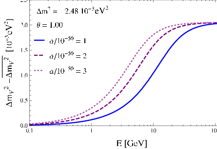
For $V=0$ the vacuum results $\sin^{2}2\theta$ and $\Delta m^{2}$ are obtained. For anti-neutrinos, the potential $V$ and hence $\eta$ changes sign, thereby an apparent difference between the oscillation parameters of neutrinos $(\Delta m^{2}_{V},\theta)$ and anti-neutrinos $(\overline{\Delta m^{2}_{V}},\overline{\theta})$ could arise. Fig. 2 shows the difference between the mass-squared differences of neutrinos and anti-neutrinos (choosing an initial value of $\mbox{$\Delta m^{2}$}=-2.48\times 10^{-3}$ eV²) for different values of $\alpha$ as a function of energy.

We note here three important properties following from Eqs. (40, 41):

• •

  first, the effect goes with $\eta\,\cos 2\theta$, and therefore it is absent if $\theta$ is maximal. In this case the oscillation parameters $\theta$ and $\Delta m^{2}$ would be the same for neutrinos and anti-neutrinos, but with a common offset compared to their values for $V=0$. If the long-range force mediated by $L_{\mu}-L_{\tau}$ is responsible for the MINOS anomaly, then the necessary $\theta\neq\pi/4$ is a possibility to disentangle it from any other proposed explanation [12, 13, 14];

• •

  the second point is that the corrections to the mixing angle and the mass-squared difference are correlated. For positive $\Delta m^{2}$ and $\alpha$ the correction for $\sin^{2}2\theta$ goes in the opposite direction as the correction of the $\Delta m^{2}$. Recalling that MINOS finds $\overline{\Delta m^{2}}>\Delta m^{2}$ we therefore predict for positive $\Delta m^{2}$ and $\alpha$ that $\sin^{2}2\theta>\sin^{2}2\overline{\theta}$, which is compatible with the MINOS results (see Eq. (1)), and can be checked with higher statistics data sets. For negative $\Delta m^{2}$ and positive $\alpha$ the correction goes in the same direction, and hence $\sin^{2}2\theta<\sin^{2}2\overline{\theta}$;

• •

  the third point is that the relative effect is expected to be slightly larger for $\sin^{2}2\theta$ than for $\Delta m^{2}$.

We can estimate the magnitude of the parameter $\eta$ as

$$\eta\simeq 0.025\left(\frac{\alpha}{10^{-50}}\right)\left(\frac{E}{\rm GeV}\right),$$

(42)

which allows for not too high energies (note that at MINOS the oscillation dip occurs at around $E\sim 1$ GeV) and for $\alpha$ around $10^{-50}$ (see the discussion after Eq. (18)), $\eta$ is small and can be used as an expansion parameter. As can be seen from (40) and (41) the relative difference of the mass-squared differences is in this case obtained as

$$\frac{\Delta m_{V}^{2}-\overline{\Delta m_{V}^{2}}}{\Delta m^{2}}\simeq-4\,\eta\,\cos 2\theta\,,$$

(43)

while for the mixing angle the result is:

$$\frac{\sin^{2}2\theta_{V}-\sin^{2}2\overline{\theta}_{V}}{\sin^{2}2\theta}\simeq 8\,\eta\,\cos 2\theta\,.$$

(44)

These expressions nicely confirm the three points mentioned above. The muon neutrino and anti-neutrino survival probabilities are

	$\displaystyle P\equiv P(\nu_{\mu}\rightarrow\nu_{\mu})$	$\displaystyle=1-\sin^{2}2\theta_{V}\,\sin^{2}\frac{\Delta m_{V}^{2}}{4\,E}L\,,$		(45)
	$\displaystyle\overline{P}=P(\overline{\nu}_{\mu}\rightarrow\overline{\nu}_{\mu})$	$\displaystyle=P(\nu_{\mu}\rightarrow\nu_{\mu})(\alpha\leftrightarrow-\alpha)\,,$		(46)

which are subject to the following degeneracies

$$P(\theta,\Delta m^{2},\alpha)=P(\theta,-\Delta m^{2},-\alpha)=P(\theta+\pi/2,\Delta m^{2},-\alpha)=P(\theta+\pi/2,-\Delta m^{2},\alpha)\,.$$

(47)

While the part discussed so far was rather general, we continue by applying the formalism to the recently found MINOS results [11]. We have performed with the expressions (45, 46) a $\chi^{2}$-fit to the MINOS data (given in bins of energy $E_{i}$) on the ratio of observed events divided by the expectation for no oscillations. This data was taken, as in Ref. [14], from the slides of the talk referred to in our Ref. [11]. In case of asymmetric errors, the largest one was used and inserted in the $\chi^{2}$-function

$$\chi^{2}(\theta,\Delta m^{2},\alpha)=\sum\limits_{i}\left(\frac{P(\theta,\Delta m^{2},\alpha,E_{i})-R_{i}}{\sigma_{i}^{2}}\right)^{2}+\sum\limits_{i}\left(\frac{\overline{P}(\theta,\Delta m^{2},\alpha,E_{i})-\overline{R}_{i}}{\overline{\sigma}_{i}^{2}}\right)^{2},$$

(48)

where $P$ $(\overline{P})$ is the survival probability $P(\nu_{\mu}\rightarrow\nu_{\mu})$ from Eq. (45) (from Eq. (46)), $R_{i}$ ($\overline{R}_{i}$) the ratio of observed events relative to the no-oscillation expectation, and $\sigma_{i}$ ($\overline{\sigma}_{i}$) the error for the neutrino (anti-neutrino) data set.

The result of our fit after marginalizing over $\Delta m^{2}$ and $\theta$ is⁴⁴ 4 We have checked our analysis by setting $\alpha=0$ and have obtained the best-fit values $\mbox{$\Delta m^{2}$}=2.28\times 10^{-3}$ eV², $\sin^{2}2\theta=0.94$ for the neutrino data set, and $\mbox{$\overline{\Delta m^{2}}$}=3.38\times 10^{-3}$ eV², $\sin^{2}2{\overline{\theta}}=0.81$ for the anti-neutrinos, in good agreement with the MINOS results. A fit to the total data set yields $\mbox{$\Delta m^{2}$}=(2.38^{+0.20}_{-0.17})\times 10^{-3}$ eV² and $\sin^{2}2\theta=0.89^{+0.08}_{-0.07}$, with $\chi^{2}_{\rm min}/N_{\rm dof}=49.43/51\simeq 0.97$.

$$\sin^{2}2\theta=0.83\pm 0.08~,~~\Delta m^{2}=(-2.48\pm 0.19)\times 10^{-3}\,{\rm eV}^{2}~,~~\alpha=\left(1.52_{-1.14}^{+1.17}\right)\times 10^{-50}\,,$$

(49)

with $\chi^{2}_{\rm min}/N_{\rm dof}=47.77/50\simeq 0.96$. Recall the degeneracies listed in Eq. (47). In Fig. 3 we show the experimental data together with the results of our fit.

One can see that the non-zero value of $\alpha$ puts in particular the data points at the oscillation minimum in better agreement with the curves. From the plot of the $\chi^{2}$-function in Fig. 4 one sees that there is a second (local) minimum, corresponding to $\sin^{2}2\theta=0.98$, $\Delta m^{2}=2.36\times 10^{-3}\,{\rm eV}^{2}$ and $\alpha=4.41\times 10^{-50}$, with $\chi^{2}_{\rm min}/N_{\rm dof}=48.73/50\simeq 0.97$. The curves for this point are also plotted in Fig. 3. The second local minimum also explains the “rabbit head looking” shape of the contours in $\alpha$–$\Delta m^{2}$ and $\alpha$–$\sin^{2}2\theta$ space shown in Fig. 5.

The goodness of fit is not particularly worse for the absence of new physics, which has been noted also in Ref. [14].

We continue by discussing the consequences of the implied value of $\alpha$ in future neutrino oscillation experiments. We have modified the commonly used GLoBES software [25] to include the potential $V$ from Eq. (16). Using the pre-defined packages (“AEDL files”) for the most frequently discussed future experiments, we analyzed T2K, NO$\nu$A and a neutrino factory, as listed in Table 1, to obtain future constraints on $\alpha$. The oscillation parameters we use are listed in Table 2. The result is that at $3\sigma$, $\alpha$ can be constrained to be below $11.80\times 10^{-50}$, $1.93\times 10^{-50}$ and $0.53\times 10^{-50}$, respectively. The $\chi^{2}$-functions generated by GLoBES are shown in Fig. 6.

Setting the true parameter values of $\alpha$, $\theta$ and $\Delta m^{2}$ (and their errors) to our best-fit values from Eq. (49), we can see how the “precision” on $\alpha$ can be improved. From the plots of $\chi^{2}$ in Fig. 7 one sees that NO$\nu$A would give $\alpha=(1.52\pm 0.27)\times 10^{-50}$, T2K would yield $\alpha=(1.52\pm 0.46)\times 10^{-50}$ and NuFact would determine very precisely $\alpha=(1.52^{+0.11}_{-0.21})\times 10^{-50}$.

As mentioned above, long-range forces generated by $L_{e}-L_{\mu,\tau}$ have been discussed before. Ref. [3] bounds $\alpha_{e\,\mu,\tau}$ by analyzing $\nu_{\mu}$ and $\nu_{\tau}$ oscillations and using atmospheric neutrino data. It is easy to see that in a two-flavor framework, the potential $V_{e\tau}=\alpha_{e\tau}\,N_{e}/R_{\rm A.U.}$ corresponds to $2\,V_{\mu\tau}$. Likewise, $V_{e\mu}$ corresponds to $-2\,V_{\mu\tau}$. Therefore, the limit of $\alpha_{e\tau}<6.4\times 10^{-52}$ obtained in Ref. [3] corresponds to $\alpha=g^{\prime}\,(\xi-s_{W}\,\chi)<8.9\times 10^{-50}$, not in conflict with our fit-result from Eq. (49). In turn, this means that not only $L_{\mu}-L_{\tau}$ could be the origin of the MINOS anomaly, but also $L_{e}-L_{\mu}$ or $L_{e}-L_{\tau}$, for which $\alpha=1.52\times 10^{-50}$ translates into $\alpha_{e\,\mu,\tau}=1.1\times 10^{-52}$. If we take the $3\sigma$-bound $\alpha_{e\tau}<2.5\times 10^{-53}$ from solar neutrino and KamLAND data [4] and treat it like in the 2-flavor case we obtain $\alpha<3.5\times 10^{-51}$. However, the interplay of the other limits on long-range forces, and also the impact of stronger bounds on $\alpha_{e\,\mu,\tau}$ using solar and KamLAND data [4], can not be used without doing a full 3-flavor fit to all data. In general, we note that the different flavor structures of the potentials arising from $L_{e}-L_{\mu}$, $L_{e}-L_{\tau}$ and $L_{\mu}-L_{\tau}$,

$$\left(\begin{array}[]{ccc}V&0&0\\ 0&-V&0\\ 0&0&0\end{array}\right)~,~~\left(\begin{array}[]{ccc}V&0&0\\ 0&0&0\\ 0&0&-V\end{array}\right)~,~~\left(\begin{array}[]{ccc}0&0&0\\ 0&V&0\\ 0&0&-V\end{array}\right),$$

(50)

render it difficult to translate existing bounds on $L_{e}-L_{\mu}$ or $L_{e}-L_{\tau}$ into constraints on $L_{\mu}-L_{\tau}$, in particular if in addition a matter potential is present in $V_{ee}$. We would like to stress though that the solar neutrino oscillations should really be fitted specifically for this model, since the electron and neutron densities in the Sun are not proportional.

References

- [1] P. Langacker, Rev. Mod. Phys. 81, 1199 (2008) [arXiv:0801.1345 [hep-ph]].
- [2] R. Foot, Mod. Phys. Lett. A 6, 527 (1991); X. G. He, G. C. Joshi, H. Lew and R. R. Volkas, Phys. Rev. D 44, 2118 (1991); R. Foot, X. G. He, H. Lew and R. R. Volkas, Phys. Rev. D 50, 4571 (1994) [arXiv:hep-ph/9401250].
- [3] A. S. Joshipura and S. Mohanty, Phys. Lett. B 584, 103 (2004) [arXiv:hep-ph/0310210].
- [4] A. Bandyopadhyay, A. Dighe and A. S. Joshipura, Phys. Rev. D 75, 093005 (2007) [arXiv:hep-ph/0610263].
- [5] J. A. Grifols and E. Masso, Phys. Lett. B 579, 123 (2004) [arXiv:hep-ph/0311141]; M. C. Gonzalez-Garcia et al., JCAP 0701, 005 (2007) [arXiv:hep-ph/0609094]; A. Samanta, arXiv:1001.5344 [hep-ph].
- [6] S. Baek, N. G. Deshpande, X. G. He and P. Ko, Phys. Rev. D 64, 055006 (2001) [arXiv:hep-ph/0104141].
- [7] S. Baek and P. Ko, JCAP 0910, 011 (2009) [arXiv:0811.1646 [hep-ph]].
- [8] N. F. Bell and R. R. Volkas, Phys. Rev. D 63, 013006 (2001) [arXiv:hep-ph/0008177]; E. Ma, D. P. Roy and S. Roy, Phys. Lett. B 525, 101 (2002) [arXiv:hep-ph/0110146].
- [9] S. Choubey and W. Rodejohann, Eur. Phys. J. C 40, 259 (2005) [arXiv:hep-ph/0411190].
- [10] W. Rodejohann and M. A. Schmidt, Phys. Atom. Nucl. 69, 1833 (2006) [arXiv:hep-ph/0507300]; B. Adhikary, Phys. Rev. D 74, 033002 (2006) [arXiv:hep-ph/0604009]; T. Ota and W. Rodejohann, Phys. Lett. B 639, 322 (2006) [arXiv:hep-ph/0605231]; E. J. Chun and K. Turzynski, Phys. Rev. D 76, 053008 (2007) [arXiv:hep-ph/0703070].
- [11]
Talk given by P. Vahle at
24th International Conference On Neutrino Physics And Astrophysics
(Neutrino 2010), June 14, 2010, slides can be found at
http://indico.cern.ch/materialDisplay.py?contribId=201&sessionId=1
&materialId=slides&confId=73981 - [12] G. Barenboim and J. D. Lykken, Phys. Rev. D 80, 113008 (2009) [arXiv:0908.2993 [hep-ph]].
- [13] N. Engelhardt, A. E. Nelson and J. R. Walsh, Phys. Rev. D 81, 113001 (2010) [arXiv:1002.4452 [hep-ph]].
- [14] W. A. Mann, D. Cherdack, W. Musial and T. Kafka, arXiv:1006.5720 [hep-ph].
- [15] K. S. Babu, C. F. Kolda and J. March-Russell, Phys. Rev. D 57, 6788 (1998) [arXiv:hep-ph/9710441].
- [16] B. Holdom, Phys. Lett. B 166, 196 (1986).
- [17] S. Schlamminger, K. Y. Choi, T. A. Wagner, J. H. Gundlach and E. G. Adelberger, Phys. Rev. Lett. 100, 041101 (2008) [arXiv:0712.0607 [gr-qc]]; E. G. Adelberger, J. H. Gundlach, B. R. Heckel, S. Hoedl and S. Schlamminger, Prog. Part. Nucl. Phys. 62, 102 (2009).
- [18] C. Amsler et al. [Particle Data Group], Phys. Lett. B 667, 1 (2008).
- [19] For a recent review, see S. Hannestad, arXiv:1007.0658 [hep-ph].
- [20] J. A. Grifols and E. Masso, Phys. Lett. B 396, 201 (1997) [arXiv:astro-ph/9610205]; L. B. Okun, Mod. Phys. Lett. A 11, 3041 (1996) [arXiv:hep-ph/9611360].
- [21] S. N. Gninenko, Phys. Lett. B 413, 365 (1997) [arXiv:hep-ph/9708465].
- [22] A. D. Dolgov, Phys. Rept. 320, 1 (1999).
- [23] X. Fei, Phys. Rev. A 49, 1467 (1994).
- [24] S. J. Brodsky and R. F. Lebed, Phys. Rev. Lett. 102, 213401 (2009) [arXiv:0904.2225 [hep-ph]].
- [25] P. Huber, M. Lindner and W. Winter, Comput. Phys. Commun. 167, 195 (2005) [arXiv:hep-ph/0407333]; P. Huber, J. Kopp, M. Lindner, M. Rolinec and W. Winter, Comput. Phys. Commun. 177, 432 (2007) [arXiv:hep-ph/0701187].
- [26] T. Schwetz, M. A. Tortola and J. W. F. Valle, New J. Phys. 10, 113011 (2008) [arXiv:0808.2016v3 [hep-ph]].
- [27] C. Biggio, M. Blennow and E. Fernandez-Martinez, JHEP 08, 090 (2009) [arXiv:0907.0097v3 [hep-ph]].
- [28] A. Friedland, C. Lunardini and M. Maltoni, Phys. Rev. D 70, 111301 (2004) [arXiv:hep-ph/0408264]; A. Friedland and C. Lunardini, Phys. Rev. D 72, 053009 (2005) [arXiv:hep-ph/0506143].
- [29] A. A. Aguilar-Arevalo et al. [The MiniBooNE Collaboration], arXiv:1007.1150 [hep-ex].