USTC-ICTS-10-08

A Matter Bounce By Means of Ghost Condensation

Chunshan Lin^1,2), Robert H. Brandenberger¹⁾ and Laurence Perreault Levasseur¹⁾ Affiliation: 1) Physics Department, McGill University, Montreal, QC, H3A 2T8, Canada Affiliation: 2) Interdisciplinary Center of Theoretical Studies, University of Science and Technology of China, Hefei, Anhui 230026, China

Abstract

Assuming the existence of a scalar field which undergoes “ghost condensation” and which has a suitably chosen potential, it is possible to obtain a non-singular bouncing cosmology in the presence of regular matter and radiation. The potential for the ghost condensate field can be chosen such that the cosmological bounce is stable against the presence of anisotropic stress. Cosmological fluctuations on long wavelengths relevant to current cosmological observations pass through the bounce unaffected by the new physics which yields the bounce. Thus, this model allows for the realization of the “matter bounce” scenario, an alternative to inflationary cosmology for the generation of the observed primordial fluctuations in which the inhomogeneities originate as quantum vacuum perturbations which exit the Hubble radius in the matter-dominated phase of contraction.

I introduction

The inflationary universe scenario [1, 2] is the current paradigm for early universe cosmology. While phenomenologically successful, inflationary models face various conceptual problems (see e.g. [3]), most notably the singularity problem [4]. Hence, it has been of great interest to construct nonsingular bouncing cosmologies (for a recent review see e.g. [5]).

It is possible that a nonsingular cosmological bounce is followed by a period of inflation (see e.g. [6] for an example). However, it is also of interest to explore alternatives to inflation which could result from a bouncing cosmology. In [7, 8] it was realized that quantum vacuum fluctuations which exit the Hubble radius in a matter-dominated phase of contraction obtain a scale-invariant spectrum of curvature fluctuations on super-Hubble scales. Provided that on the large scales corresponding to current cosmological observations the fluctuations pass through the bounce unaffected by the new physics which yields the cosmological bounce, then we have a mechanism alternative to inflation for producing a scale-invariant spectrum of cosmological perturbations. This alternative is called the “matter bounce scenario” (see e.g. [9] for introductory reviews). The matter bounce scenario can be distinguished from simple inflationary models through the shape and amplitude of the bispectrum, the three-point function of cosmological perturbations, which has a special shape and an amplitude which is large compared to what results in simple inflationary models [10].

From the Penrose-Hawking singularity theorems [11] it is clear that new physics is required in order to obtain a cosmological bounce. There have to be modifications either to the gravitational action, or else matter which violates the usual energy conditions has to be introduced. There have been various suggestions on how to obtain a cosmological bounce by means of modifying gravity. For example, the “non-singular Universe” construction of [12] yields a cosmological bounce, as does the ghost-free higher derivative gravity action of [13]. It is also possible to obtain a bounce in the context of “mirage cosmology” where our space-time is a brane moving in a curved higher-dimensional background space [14]. As was realized in [15], in the presence of spatial curvature a cosmological bounce also occurs generically in Hořava-Lifshitz gravity [16].

If we maintain General Relativity as the theory of space-time, then a cosmological bounce can also occur if we suitably modify the matter sector. A generic way of obtaining a bounce is to add to the usual matter sector which obeys the standard energy conditions a “ghost” sector with opposite sign kinetic energy terms in the matter Lagrangian. This class of models is called “quintom” models [17] and can lead to a bounce [18]. One way to realize a quintom bounce is by considering a scalar field $\varphi$ with standard kinetic term and with mass $m$ and adding a ghost scalar field $\tilde{\varphi}$ with mass $M\gg m$ . This model was considered in detail in [19]. A specific realization is in the context of the scalar field sector of the Lee-Wick Standard Model [20], as studied in [21]. A serious challenge for all models with a ghost field is the ghost instability problem (see e.g. [22]).

All analyses of the evolution of cosmological fluctuations through non-singular bounces (e.g. [23] in the case of the model of [13], [14] in the case of a mirage cosmology bounce, [19, 21] in the case of quintom models and [24] in the case of the Hořava-Lifshitz bounce) indicate that the spectrum of the curvature fluctuations does not change during the bounce phase on length scales larger than the duration of the bounce.

There are two serious problems for matter bounce scenarios. The first is the fact that some bounces are unstable to the presence of radiation, the reason being that the energy density of radiation increases faster as the universe contracts compared to the increase in the effective energy in the terms yielding the bounce. In particular, this was shown [25] to be a serious problem in the case of the bounce in the Lee-Wick model, and the problem will likely also be serious in other models in which the ghost field yielding the bounce is a scalar field. In contrast, models which are based on asymptotically free gravity models such as [12] and [13] will be free from this problem, as is the bounce in Hořava-Lifshitz gravity.

An even more serious problem is the instability of the contracting pre-bounce phase to the presence of anisotropies since the energy density in anisotropies scales as $a^{-6}$ ( $a(t)$ being the cosmological scale factor) compared to $a^{-4}$ for radiation ¹¹ 1 This leads to the BKL [26] chaotic behavior at the “Big Crunch” singularity.. This implies that the cosmological bounce cannot be described in terms of a homogeneous and isotropic background.

In this paper, we present a ghost condensation model in which a cosmological bounce can be obtained. Since there is no ghost in the perturbative spectrum of the theory, the model is free from the ghost instability problem of [22]. The model is also free from the two problems we just mentioned above. The effective equation of state of the ghost condensate is $w>1$ and hence, as studied in [27] in the context of the Ekpyrotic scenario [28], the anisotropies do not come to dominate and the cosmological background remains well described in terms of a homogeneous and isotropic metric.

Ghost condensation was proposed [29] as a theoretically consistent modification of gravity in the infrared. It is based on the analog of the Higgs mechanism in the kinetic sector of a scalar field Lagrangian. The kinetic term $X$ of the scalar field $\phi$ , i.e.

X\,\equiv\,-g^{\mu\nu}\partial_{\mu}\phi\partial_{\nu}\phi\,

(1)

where we are choosing the metric signature to be (-, + + +), appears in the Lagrangian in terms of a function $P(X)$ with a nontrivial minimum, such that the leading term in $X$ in the Lagrangian has the “wrong” sign, i.e. appears as a ghost. If the function $P(X)$ has a non-trivial minimum at $X=c^{2}$ (the “ghost condensate”) and the field configuration takes on this value, then fluctuations about this configuration have normal kinetic term. Thus, there is no ghost in the spectrum of fluctuations about the ghost condensate.

It was soon realized that, although initially introduced [29] to provide a new explanation for infrared effects in gravity, the ghost-condensation mechanism has many applications in cosmology at ultraviolet scales. For example, it can be used [30] to provide a new mechanism for inflation. It was realized in [31] that the ghost condensate mechanism can also provide stable violations of the null energy condition and thus used to construct non-standard cosmologies, including bouncing ones. Ghost condensation was used in [32, 33] to provide non-singular versions of Ekpyrotic cosmology. In this paper we make use of the ghost condensation mechanism to construct a non-singular matter bounce.

The outline of the paper is as follows. In the following section we briefly review the idea of ghost condensation. In Section 3 we work out the requirements for the ghost field potential $V(\phi)$ in order to obtain a bounce, in particular a bounce which is stable against the addition of radiation and anisotropic stress. In Section 4 we discuss the transfer of cosmological fluctuations through the ghost bounce phase. The final section contains our conclusions and a discussion of the results.

To set the notation, we work in terms of a spatially flat Friedmann-Robertson-Walker background with metric

ds^{2}\,=\,-dt^{2}+a(t)^{2}(dx^{2}+dy^{2}+dz^{2})\,,

(2)

where $a(t)$ is the scale factor, $t$ is the physical time and $x,y$ and $z$ are the co-moving spatial coordinates. The Hubble expansion rate is $H(t)=\dot{a}/a$ .

II Ghost Condensation

The Lagrangian of ghost condensation takes the following general form

\mathcal{L}\,=\,M^{4}P(X)-V(\phi)\,,

(3)

where $M$ is the characteristic mass scale of ghost condensation and we follow the usual convention in the ghost condensation literature to take $\phi$ to have dimensions of length such that $X$ is dimensionless. To obtain a ghost condensate, the function $P(X)$ must have a non-trivial minimum. To avoid a cosmological constant problem, we set the value of $P$ at the minimum to be zero. We will use the prototypical example

P(X)\,=\,\frac{1}{8}(X-c^{2})^{2}\,,

(4)

where $c$ is a dimensionless constant which has nothing to do with the speed of light (we are following the notation of the original papers on ghost condensation). The ghost condensate necessarily breaks Lorentz invariance. The homogeneous and isotropic ground state corresponds to the background scalar field configuration

\phi\,=\,ct\,.

(5)

The equation of motion of the ghost condensation field is

(P^{\prime}+2\dot{\phi}^{2}P^{\prime\prime})\ddot{\phi}+3HP^{\prime}\dot{\phi}\,=\,-M^{-4}\frac{\partial V}{\partial\phi}~,

(6)

where $P^{\prime}\equiv\frac{\partial P}{\partial X}$ .

The analogs of the Friedmann equations obtained by coupling the homogeneous and isotropic ghost condensate to Einstein gravity are

3M_{p}^{2}H^{2}\,=\,M^{4}\bigl(2XP^{\prime}-P\bigr)+V+\rho_{m}\,,

(7)

and

2M_{p}^{2}\dot{H}\,=\,-2M^{4}XP^{\prime}-(1+w_{m})\rho_{m}\,.

(8)

We have assumed that in addition to the ghost condensate, there is also regular matter with energy density $\rho_{m}$ and equation of state $w=w_{m}$ , where $w$ is the ratio of pressure density to energy density.

Let us now consider homogeneous fluctuations $\pi$ about the ghost condensate field, i.e.

\phi(t)\,=\,ct+\pi(t)\,.

(9)

Inserting into (7) and (8) we obtain the following expressions for the energy and pressure densities of the homogeneous $\pi$ field:

	$\displaystyle\rho_{X}\,$	$\displaystyle=$	$\displaystyle\,M^{4}c^{3}\dot{\pi}\bigl(1+{\cal{O}}(\frac{\dot{\pi}}{c})\bigr)+V\,,$		(10)
	$\displaystyle\rho_{X}+p_{X}\,$	$\displaystyle=$	$\displaystyle\,M^{4}c^{3}\dot{\pi}\bigl(1+{\cal{O}}(\frac{\dot{\pi}}{c})\bigr)\,.$		(11)

In order to obtain a cosmological bounce, it is necessary to cancel the positive energy density of regular matter with the negative energy density of the ghost condensate. This can be achieved by having negative ${\dot{\pi}}$ . To complete the system of equations for the fluctuations of the ghost condensate, we write down the variational equation with respect to $\phi$ . To leading order in ${\cal{O}}(\frac{\dot{\pi}}{c})$ it is

c^{2}a^{-3}\partial_{t}\bigl(a^{3}{\dot{\pi}}\bigr)\,=\,-2M^{-4}\frac{\partial V}{\partial\phi}\,.

(12)

By inserting the ansatz (9) into the Lagrangian (3) it follows that $P^{\prime}+2\dot{\phi}^{2}P^{\prime\prime}\gg 0$ is the necessary condition for the theory expanded about the condensate to be ghost free.

III Bounce Induced by a Ghost Condensate

In the absence of regular matter, a ghost condensate leads to a cosmological bounce if the ghost field potential energy (which we assume to be positive) is cancelled by the negative ghost condensate energy. To leading order in ${\cal{O}}(\frac{\dot{\pi}}{c})$ the condition for the bounce point is

M^{4}c^{3}\dot{\pi}\,=\,-V\,.

(13)

The second Friedmann equation, i.e. (8), then implies that $\dot{H}>0$ at the bounce point, i.e. the scale factor indeed makes a transition from a contracting phase to an expanding phase.

To obtain a bounce, it is necessary to have a non-trivial potential $V(\phi)$ since in the absence of a potential the equation of motion (12) implies

a^{3}\dot{\pi}\,=\,\rm{const}

(14)

and hence the bounce condition, which in the absence of a potential is $\dot{\pi}=0$ , cannot be reached.

To obtain a matter bounce, we must consider the equations of motion in the presence of regular matter. We assume that the universe begins at very large negative times with the ghost condensate in its ground state $X=c^{2}$ (or $\pi=0$ ). The energy density in regular matter increases in time as

\rho_{m}(t)\,\sim\,a(t)^{-3(1+w_{m})}\,.

(15)

We are interested in the cases of cold matter ( $w_{m}=0$ ) and radiation ( $w_{m}=1/3$ ), or in anisotropic stress for which $w_{m}=1$ . From (14) it follows that in the absence of a potential $V$ for $\phi$

\rho_{X}\,\sim\,a^{-3}\,.

(16)

Hence, the ghost energy density cannot catch up with the matter energy density and no bounce is possible. Thus we conclude that, as in the case without matter, also in the presence of matter it is necessary to introduce a potential $V(\phi)$ in order to obtain a bounce.

In order to obtain a bounce, the energy density in the ghost field must increase sufficiently fast:

\rho_{X}\,\sim\,a(t)^{-p}\,,

(17)

where $p>3$ is the minimal requirement, $p>4$ is required if the bounce is to be stable against the presence of regular relativistic radiation, and $p>6$ is required if the bounce is to be stable against the presence of anisotropies.

In order for the ghost energy density to increase faster than $a^{-3}$ , we require

\partial_{t}\bigl(a^{3}\dot{\pi}\bigr)\,<\,0

(18)

and hence from (12)

\frac{\partial V}{\partial\phi}\,>\,0\,.

(19)

We assume that the ghost field $\phi$ starts at large negative values. Hence, we make the following ansatz for our potential

V(\phi)\,=\,V_{0}M^{-\alpha}\phi^{-\alpha}\,,

(20)

where $V_{0}$ is a constant with units of potential energy density which sets the overall scale of the ghost energy density, and $\alpha$ is a constant to be determined by the requirement that the ghost energy density increases sufficiently fast. This potential diverges at $\phi=0$ . However, we know that the ghost condensate Lagrangian should only be trusted at energy scales lower than $M^{4}$ . Hence, we will assume that the divergence of the potential is cut off when the potential reaches this value. For example, we can assume that the potential tends smoothly to the limiting value $M^{4}$ which is taken on at $\phi=0$ (see Fig. 1 for a sketch of this potential).

Refer to caption — Figure 1: Sketch of the effective potential of the ghost condensate field.

Let us now derive the condition on $\alpha$ for which a non-singular bounce which is stable even in the presence of anisotropies will arise. For this, we return to the equation of motion (12) which after inserting the ghost fluctuation ansatz (9) and expanding to leading order in $\dot{\pi}$ becomes

c^{2}\partial_{t}\bigl(a^{3}\dot{\pi}\bigr)=-2a^{3}M^{-4-\alpha}\frac{\partial V}{\partial\phi}\,.

(21)

Inserting the form of the potential (20), the ansatz for the field $\phi$ from (9), and working in the range of times for which $|ct|\gg|\pi|$ yields

\ddot{\pi}+3H\dot{\pi}\,=\,2c^{-2}V_{0}M^{-4-\alpha}\alpha(ct)^{-(\alpha+1)}\,.

(22)

We want to derive the condition on $\alpha$ such that in a background dominated by matter with an equation of state parameter $w$ , the energy density of the ghost kinetic term which is proportional to $\dot{\pi}$ increases faster than the energy density in matter as the universe contracts. Hence, we insert the following form of the scale factor

a(t)\,=\,(\frac{-t}{t_{0}})^{2/(3(1+w))}

(23)

into (22). We see that the source term (the right hand side of (22) leads to

\dot{\pi}\,\sim\,t^{-\alpha}\,.

(24)

and the condition for the ghost kinetic energy density to grow faster than the matter energy density is

\alpha\,>\,2\,.

(25)

Since we wish the potential to be an even function of $\phi$ , we can choose $\alpha=4$ . In this case the model is marginally stable against the addition of anisotropic stress. The case $\alpha=6$ would provide a model which is stable.

Let us now summarize the evolution of the background cosmology in our ghost bounce model. We begin at $t\rightarrow-\infty$ in a contracting, matter-dominated phase with ghost condensate field $\phi\rightarrow-\infty$ and the ghost condensate in its ground state with $\pi=0$ . The energy density of the universe is initially dominated by non-relativistic matter. As the universe contracts, first radiation with $w=1/3$ and then anisotropic stress with $w=1$ take over. However, the energy density in the ghost condensate grows faster than any of these energy densities and, at some point sufficiently close to $t=0$ begins to dominate. Note that both the negative energy of the ghost kinetic term and the positive potential energy of the ghost field increase at the same rate. Eventually the ghost field $\phi$ reaches the value when the potential flattens out. At this point, the negative kinetic contribution to the ghost energy catches up, and the bounce point $H=0$ is reached. Since at this point $\dot{\pi}<0$ we have $\dot{H}>0$ and the universe begins to expand. The ghost field evolves to positive values, and both the ghost potential and kinetic energies begin to decrease rapidly, allowing the energy densities of anisotropic stress, radiation and cold matter to dominate again.

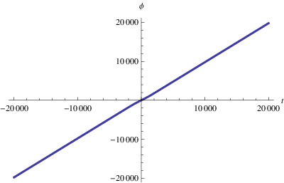
The evolution of the background has been studied numerically and the results are presented in Figures 2 - 5. In all four figures, the horizontal axis is time in Planck units. The vertical axis is $\phi$ , $\dot{\phi}$ , and $H$ respectively. There is a nonsingular bounce at time $t=0$ . The graphs are based on solving Eqs. (6) and (7) using Mathematica, beginning the evolution at the bounce point $t=0$ where “initial” conditions (again in Planck units) $\phi(0)=0$ and $\dot{\phi}(0)=\sqrt{2/3}$ are chosen. The value of $M$ was taken to be $M=2\times 10^{-3}$ , and the potential was taken to correspond to $\alpha=4$ , with a value of $V_{0}$ such that

V(\phi)\,=\,\frac{1}{\phi^{4}+10^{12}}\,.

(26)

The energy density of matter sector was taken to be $\rho_{m}(0)=10^{-12}$ . As is obvious from the graphs, a smooth nonsingular bounce results.

IV A First Look at Cosmological Perturbations in the Ghost Condensate Model

IV.1 Generating a Scale-Invariant Spectrum

In this section, we will show that the perturbations induced by the ghost condensate do not change the primordial spectrum of curvature fluctuations induced by regular matter in the contracting phase. Thus, in the matter bounce background the scale-invariant spectrum of fluctuations on scales which exit the Hubble radius during the mater-dominated phase of contraction will not be distorted by the ghost condensate, neither in the contracting nor in the bounce phase. First, in this subsection, we review how a scale-invariant spectrum of curvature fluctuations arises in the matter bounce scenario.

To set the framework, we present in Figure 6 a space-time sketch of a matter bounce. The horizontal axis is space, the vertical axis is time, and the bounce time is $t=0$ . We are interested in fluctuations on scales which are currently observable, and assume that these scales exit the Hubble radius in a matter-dominated phase of contraction. This assumption is not very restrictive. If the bounce cosmology background is time-symmetric and the expanding phase corresponds to our currently observed universe, then the assumption is satisfied for all scales on which the primordial matter power spectrum is currently well measured ²² 2 This background predicts a kink in the matter power spectrum on scales which can be probed by Lyman $\alpha$ observations - see [34] for a discussion of this point.. If the bounce is not time-symmetric, then according to the Second Law of Thermodynamics the expanding phase will have more entropy than the initial collapsing one and the radiation phase is shorter than in the case of the symmetric bounce, which means that a wider range of scales exits the Hubble radius in the matter-dominated phase.

As shown in the Figure, scales of cosmological interest today exit the Hubble radius during the matter-dominated phase of contraction. If the bounce takes place at an energy scale comparable to that of Grand Unification, then the current Hubble radius corresponds to a physical length of about $1{\rm{mm}}$ at the bounce. This scale is in the far infrared compared to the scale which sets the physics of the bounce.

The theory of cosmological perturbations in the model with both regular matter and a ghost condensate in general FRW background was worked out in [35]. Our goal here is to show that the presence of the ghost condensate and its induced curvature fluctuations will not mess up the scale-invariant spectrum of perturbations resulting from regular matter in a matter-dominated phase of contraction. We have to show first that the ghost fluctuations in the matter-dominated phase of contraction do not grow faster than the fluctuations without the presence of the ghost field. Secondly, we need to show that the curvature fluctuations which are induced by the coupling between regular matter and the ghost field are negligible, and thirdly, we need to show that the spectrum of fluctuations on scales of relevance to current cosmological observations is not changed during the short phase where the ghost condensate dominated the dynamics.

We begin with the general framework of metric fluctuations. Working in in longitudinal gauge (see [36] for a comprehensive review of the theory of cosmological perturbations) the metric including scalar fluctuations take the form

ds^{2}\,=\,-(1+2\Phi)dt^{2}+a(t)^{2}(1-2\Psi)d{\bf x}^{2}\,,

(27)

where $\Phi$ and $\Psi$ are the two gravitational potentials which depend on space and time and encode the metric perturbations. Since there is no anisotropic stress at linear order (both in the regular matter sector and in the ghost matter Lagrangian), we have $\Psi=\Phi$ as a consequence of the perturbed off-diagonal spatial Einstein equations. The remaining potential $\Phi$ is the relativistic generalization of the Newtonian gravitational potential.

To describe fluctuations on super-Hubble scales, it is more convenient to use the fluctuation variable $v$ in terms of which the action for canonical fluctuations has canonical form [37]. If matter is a simple scalar field $\varphi$ , then $v$ can be expressed in terms of the matter and metric fluctuations $\delta\varphi$ and $\Phi$ via

v\,=\,a\bigl[\delta\varphi+\frac{z}{a}\Phi\bigr]\,

(28)

where $z$ is a function of matter and metric background whose form does not concern us here (see [36] or [38] for an introductory review). Closely associated with $v$ is the variable ${\zeta}$ , the curvature fluctuation in co-moving gauge (called unitary gauge in the ghost condensate literature):

\zeta\,=\,a^{-1}v\,.

(29)

In an expanding universe the dominant of the two modes of $\zeta$ has constant amplitude. However, in a contracting universe the dominant mode of $\zeta$ is increasing on super-Hubble scales. In fact, in a matter-dominated phase of contraction the dominant mode of $v$ scales as (see [7, 8] for the original works and [9] for recent reviews)

v(t)\,\sim\,t^{-1/3}\,,

(30)

and hence

\zeta(t)\,\sim\,t^{-1}\,.

(31)

The above is exactly the growth rate needed to convert an initial vacuum spectrum for fluctuations on sub-Hubble scales into a scale-invariant spectrum on super-Hubble scales. We briefly review the argument. The vacuum spectrum for the canonical fluctuation variable states that

v(k,t)\,\sim\,k^{-1/2}

(32)

on sub-Hubble scales in the contracting phase. The condition for the time $t_{H}(k)$ when the scale $k$ crosses the Hubble radius is

t_{H}(k)\,=\,k^{-1}a(t_{H}(k))\,.

(33)

Making use of the scaling (31), the vacuum initial conditions (32) which hold until Hubble radius crossing, and the Hubble radius crossing condition (33) we obtain

\zeta(k,t)\,=\,\frac{t_{H}(k)}{t}a(t_{H}(k))v(k,t_{H}(k))\,\sim\,t_{H}(k)^{1/3}v(t_{H}(k))\,\sim\,k^{-1}k^{-1/2}\,,

(34)

which corresponds to a scale-invariant power spectrum. Note that in the last step we have used the scaling $t_{H}(k)\sim k^{-3}$ which holds in a matter-dominated phase of contraction.

Thus, we have shown that vacuum fluctuations which exit the Hubble radius during a matter-dominated phase of contraction acquire a scale-invariant spectrum of perturbations on super-Hubble scales. This spectrum is maintained if the background equation of state changes when radiation starts to dominate. We will have to show that the presence of a ghost condensate does not change the evolution of the fluctuations in the contracting phase, and that the spectrum is not distorted in the phase dominated by a ghost condensate.

IV.2 The Evolution of Ghost Perturbations

Let us now turn to the ghost matter sector. Introducing a fluctuating field $\pi(t,{\bf x})$ which depends both on space and time, the Lagrangian to quadratic order in $\pi$ about a non-trivial background $\dot{\pi_{0}}$ (the $\dot{\pi}$ appearing in the previous section) is [31]

{\cal L}\,=\,\frac{1}{2}M^{4}\dot{\pi}^{2}+\dot{H}M_{pl}^{2}(\nabla\pi)^{2}-\frac{1}{2}{\tilde{M}}^{2}(\nabla^{2}\pi)^{2}\,,

(35)

where $\nabla$ is the spatial gradient operator. Note that to leading order in $\pi$ , no quartic order spatial gradient terms appear if we only use the Lagrangian (3), and to obtain (35) we had to introduce higher derivative terms, following [29, 31]. To derive the form of the second term in (35), we made use of the ghost background equations of the previous section.

By working in unitary gauge in which $\zeta$ appears directly as the fluctuation of the diagonal term in the spatial metric, it was shown in Section 3.3 of [31] that for long wavelength modes

{\dot{\zeta}}\,\sim\,a^{-3}\,\sim\,t^{-2}\,,

(36)

where we have used the matter-dominated scaling of $a(t)$ in the last step. By comparing (31) and (36) we see that the matter and ghost-induced fluctuations grow at the same rate on large scales.

To show that the presence of a ghost condensate sector will not change the dominant contribution to the spectrum of cosmological fluctuations in the phase before the ghost condensate begins to dominate, we need to study the spectrum of the metric fluctuations induced by the presence of coupling between the matter and ghost sector. To do this, we make use of the equations for the metric fluctuation variable $\Phi$ which were derived in [35].

As matter we consider a ghost condensate in addition to a matter fluid, and we focus on a matter-dominated contracting background. Thus, the Einstein equations are

\displaystyle M_{pl}^{2}G_{\mu\nu}\,=\,T^{(\phi)}_{\mu\nu}+T_{\mu\nu}~,

(37)

where we use a superscript $(\phi)$ to denote the ghost condensate part. We split $\Phi$ into the contribution $\Phi_{m}$ which would be obtained in the absence of matter fluid, and a term $\Phi_{g}$ which is induced by the presence of the ghost:

\Phi\,=\,\Phi_{m}+\Phi_{g}\,.

(38)

If we neglect the anisotropic stress and entropy perturbation, the general equations of motion for $\Phi$ are [35]

	$\displaystyle\partial_{t}\Phi_{g}+H\Phi_{g}$	$\displaystyle=$	$\displaystyle\frac{\alpha}{2}\frac{\mathbf{k}^{2}}{a^{2}}\chi$
	$\displaystyle\partial_{t}\chi$	$\displaystyle=$	$\displaystyle\bigl(\frac{M^{2}}{M_{pl}^{2}}-\frac{2}{M^{2}}\frac{\mathbf{k}^{2}}{a^{2}}\bigr)\Phi_{g}+S_{\chi}\,,$		(39)

where $\alpha={\tilde{M}}^{2}/M^{2}$ and the source term is given by

	$\displaystyle M_{pl}^{2}\frac{\mathbf{k}^{2}}{a^{2}}S_{\chi}$	$\displaystyle=$	$\displaystyle\frac{M^{2}}{2M_{pl}^{2}}\delta\rho~,$
	$\displaystyle\frac{\mathbf{k}^{2}}{a^{2}}\Phi_{m}$	$\displaystyle=$	$\displaystyle\frac{\delta\rho}{2M_{pl}^{2}}~.$		(40)

Note that the two equations in (39) come from combining all of the perturbed Einstein equations, i.e. the $0-0$ , $0-i$ , and $i-i$ components. Thus, the set of these equations is complete. Combining these two equations we obtain the following equation of motion for the Newtonian potential:

\displaystyle\partial_{t}^{2}\Phi_{g}+3H\partial_{t}\Phi_{g}+(2H^{2}+\dot{H})\Phi_{g}+\frac{\alpha}{M^{2}}\left(\frac{\mathbf{k}^{2}}{a^{2}}\right)^{2}\Phi_{g}-\frac{\alpha M^{2}}{2M_{pl}^{2}}\frac{\mathbf{k}^{2}}{a^{2}}\Phi_{g}\,

\displaystyle=

\displaystyle\,\frac{\alpha}{2}\frac{M^{2}}{M_{pl}^{2}}\frac{\mathbf{k}^{2}}{a^{2}}\Phi_{m}\,.

(41)

This equation can be simplified by factoring out the expansion/contraction of space via defining the new variable $\tilde{\Phi}=a(t)\Phi$ , and by working with conformal time $\tau$ defined via $dt=a(t)d\tau$ . Then, the equation of motion for the Newtonian potential can be rewritten as

\displaystyle\tilde{\Phi}_{g}^{\prime\prime}+\frac{81\alpha}{M^{2}}\frac{\mathbf{k}^{4}t_{0}^{4}}{\tau^{4}}\tilde{\Phi}_{g}-\frac{\alpha M^{2}}{2M_{pl}^{2}}\mathbf{k}^{2}\tilde{\Phi}_{g}

\displaystyle=

\displaystyle\frac{\alpha}{2}\frac{M^{2}}{M_{pl}^{2}}\mathbf{k}^{2}\tilde{\Phi}_{m}~,

(42)

where a prime indicates the derivative with respect to $\tau$ . We have already used the matter contracting background $a=\frac{t}{t_{0}}^{2/3}$ (where $t_{0}$ is some reference time) to get the above equation.

We will solve (42) in the large wavelength approximation in which we neglect the $k^{4}$ term. Then, the general solution is a combination of the general solution $\Phi_{g}^{h}$ of the homogeneous equation and a particular solution $\Phi_{g}^{p}$ of the inhomogeneous equation which can be determined by the Green function method. To simplify the notation we introduce the constants where

	$\displaystyle\beta\,$	$\displaystyle\equiv$	$\displaystyle\,\frac{81\alpha}{M^{2}}~,$
	$\displaystyle\gamma\,$	$\displaystyle\equiv$	$\displaystyle\,\frac{\alpha M^{2}}{2M_{pl}^{2}}$		(43)

The general solution of the homogeneous equation is

\tilde{\Phi}_{g}^{h}\,=\,c_{1}e^{k\sqrt{\gamma}\tau}+c_{2}e^{-k\sqrt{\gamma}\tau}\,,

(44)

where $c_{1}$ and $c_{2}$ are constants which multiply the two basis solutions of the equation $C_{1}(\tau)$ and $C_{2}(\tau)$ , respectively. The Wronskian $\epsilon(\tau)$ obtained from the two basis solutions is

\epsilon(\tau)\,=\,(2k\sqrt{\gamma})^{-1}

(45)

in terms of which the particular solution $\Phi_{g}^{p}$ becomes

\tilde{\Phi}_{g}^{p}(\tau)\,=\,C_{1}(\tau)\int d\tau^{{}^{\prime}}\epsilon(\tau^{{}^{\prime}})C_{2}(\tau^{{}^{\prime}}){\cal{S}}(\tau^{{}^{\prime}})-C_{2}(\tau)\int d\tau^{{}^{\prime}}\epsilon(\tau^{{}^{\prime}})C_{1}(\tau^{{}^{\prime}}){\cal{S}}(\tau^{{}^{\prime}})\,,

(46)

where ${\cal{S}}(\tau)$ is the source term in (42). Recall that the general solution for $\Phi_{m}$ on super Hubble scales [8] is

\displaystyle\tilde{\Phi}_{m}\,=\,a(t)\Phi_{m}\,=\,D\tau^{2}+\frac{S}{\tau^{3}}~,

(47)

where $D$ and $S$ are constants. Inserting this equation into the source term in (42), and approximating the mode functions $C_{1}(\tau)$ and $C_{2}(\tau)$ of the homogeneous equations as constant (which is justified over short time intervals for long wavelength modes), we obtain the following approximate form for the particular solution

\tilde{\Phi}_{g}^{p}(\tau)\,\simeq\,k^{2}\gamma\tau\bigl(\frac{D}{3}\tau^{3}-\frac{S}{2}\tau^{-2}\bigr)\,.

(48)

Note that the effects of the $k^{4}$ term in the equation of motion (42) can be included to leading order using the Born approximation. In this approximation, the contribution to $\tilde{\Phi}_{g}$ induced by the $k^{4}$ term is obtained by taking the $k^{4}$ term to the right-hand side of (42), evaluating it for the homogeneous solution $\tilde{\Phi}_{g}^{h}$ , and using it as a second source term in (46) to obtain a second contribution to the particular solution. This source term scales as $\tau^{-4}$ , and hence its contribution to $\tilde{\Phi}_{g}^{p}$ will scale as $\tau^{-2}$ , it also grows slower than $\tilde{\Phi}_{m}$ . On the other hand, the spectrum is suppressed by a factor of $k^{3}$ and is thus highly blue and completely negligible on scales relevant to current cosmological observations.

Returning to the contribution to $\tilde{\Phi}_{g}^{p}$ which dominates on large scales, we conclude that on super-Hubble scales the leading term comes from $\tilde{\Phi}_{g}^{p}$ and is

\displaystyle\Phi_{g}\,\sim\,a(t)^{-1}\tilde{\Phi}_{g}\,\sim\,\frac{k^{2}\gamma S}{\tau^{3}}.

(49)

Comparing with the matter perturbation

\Phi_{m}\sim\frac{S}{\tau^{5}}\,,

(50)

we see that the perturbation spectrum of the terms generated by the ghost condensate is blue, and that it grows more slowly than the contribution from the matter sector. This is a self consistent result. As analyzed at the beginning of this section, the spectrum of the perturbations induced by matter is scale-invariant because the amplitude of the perturbations which cross the Hubble radius at an earlier time grows and catches up to the amplitude of the perturbations which cross the Hubble radius at a later time in the contracting phase. Since the perturbation induced by the ghost condensate grows slower than that induced by matter, the perturbations which cross the Hubble radius at an earlier time cannot catch up to the amplitude of the perturbations which cross the Hubble radius at a later time, and thus the spectrum is blue. The scale-invariant spectrum of the perturbations induced by matter will be preserved in the contracting phase.

The third step is to show that the spectrum remains unchanged around the bounce phase. We only need to show that the amplitude of the curvature fluctuation induced by the ghost condensate will not grow too much during the bounce phae. This can be seen easily from Eq.(41). Since the duration of bounce phase is very short and scale factor $a(t)$ is almost a constant we can parameterize the background as follows:

\displaystyle H\,=\,\theta\cdot(t-t_{B})~,

(51)

where $t_{B}$ is the time at the bounce point, and $\theta$ is a constant with $\theta\gg H_{c}^{2}$ , where $H_{c}$ is the value of $H$ at the matching surface between the contracting phase and the bounce phase ³³ 3 Note that this implies that the duration $\delta t$ of the bounce phase satisfies $\sqrt{\theta}\delta t\ll 1$ . . On scales of interest to current observations we have $\frac{k^{2}}{a^{2}}\ll H_{c}^{2}\ll\theta$ , and thus Eq.(41) can be rewritten as

\displaystyle\partial_{t}^{2}\Phi_{g}+\theta\Phi_{g}\,=\,0~,

(52)

the solution of which is

\Phi_{g}\,=\,d_{1}e^{i\sqrt{\theta}t}+d_{2}e^{-i\sqrt{\theta}t}\,.

(53)

Since the bounce phase is so short we thus have

\Phi_{g}(t)\,\simeq\,\Phi_{g}^{c}

(54)

also at the end of the bounce phase (where $\Phi_{g}^{c}$ is the Newtonian potential induced by the ghost condensate at the beginning of the bounce phase). The perturbation induced by the ghost is almost the same as at the end of the contracting phase.

Note that near the bounce point the perturbation re-enters the Hubble radius for a very brief time interval, but $k^{2}\ll\theta$ is still true since scale factor is almost a constant during the bounce phase, and thus Eq. (52) is still valid for describing the perturbations near bounce point. We thus see that, as long as the perturbations induced by the ghost are unimportant during the contracting phase, they will also be unimportant during the bounce phase.

Previous work in the context of a wide range of non-singular bouncing models (see e.g. [14, 19, 21, 23, 24]) has shown that the matter-induced fluctuations do not change during the bounce phase. Thus, we conclude that the full spectrum of cosmological perturbations in our model does not change during the bounce phase.

IV.3 Stability of Ghost Perturbation

As derived in Section 3.3 of [31], the action for the curvature fluctuation variable $\zeta$ is

S\,=\,\int d^{3}xdta^{3}(t)\bigl[A(t){\dot{\zeta}}^{2}+B(t)(\frac{\nabla\zeta}{a})^{2}+C(t)(\frac{\nabla^{2}\zeta}{a^{2}})^{2}\bigr]\,,

(55)

where the coefficient functions $A(t),B(t)$ and $C(t)$ are given in the Appendix. Near the bounce point we can take the scale factor to be a constant and neglect the terms proportional to $H$ which appear in the coefficient functions. Then, for each Fourier mode we obtain a harmonic oscillator equation, and the dispersion relation is

\omega^{2}\,=\,\frac{-(\tilde{M}^{2}M^{4}+4M_{pl}^{4}{\dot{H}})k^{2}+2M_{pl}^{2}{\tilde{M}}^{2}k^{4}}{2M_{pl}^{2}M^{4}}\,.

(56)

As is obvious from (56), there is an instability for all long wavelength modes. In fact, the instability is a combination of two instabilities which can be seen [29, 31] at a heuristic level, the first being a gradient instability which appears if $\dot{H}>0$ as it is near the bounce, and the second a Jeans type instability. These are due to the second and first terms, respectively, in the coefficient of the $k^{2}$ term in (56). It is easy to determine the value of $k$ for which the instability is the strongest. The exponent $\omega_{c}$ of the instability is

\omega_{c}\,=\,\frac{1}{4}\frac{\tilde{M}M^{2}}{M_{pl}^{2}}+\dot{H}\frac{M_{pl}^{2}}{M^{2}\tilde{M}}\,.

(57)

We will now argue that the bounce period is too short for this instability to change the spectrum of cosmological perturbations. To estimate the time period $\Delta t$ of the bounce, we use

\Delta t\dot{\phi}\,=\,\Delta\phi\,,

(58)

where $\Delta\phi$ is the interval of $\phi$ corresponding to the bounce. We will estimate this distance by the field value for which the potential (20) approaches its maximal value which we take to be $V(\phi)=M^{4}$ . This gives

\Delta\phi\,\sim\,M^{-1}\bigl(\frac{V_{0}}{M^{4}}\bigr)^{1/\alpha}\,.

(59)

Inserting $\dot{\phi}\simeq c$ and setting the constant $c=1$ we obtain

\Delta t\omega_{c}\,\sim\,\bigl(\frac{V_{0}}{M^{4}}\bigr)^{1/\alpha}\bigl[\frac{1}{4}\frac{\tilde{M}M}{M_{pl}^{2}}+\dot{H}\frac{M_{pl}^{2}}{M^{3}\tilde{M}}\bigr]\,.

(60)

The first term in the square bracket is clearly much smaller than one. To estimate the value of the second term, we make use of (8) and (11) to estimate the value of $\dot{H}$ :

\dot{H}\,\sim\,\frac{M^{4}\dot{\pi}}{M_{pl}^{2}}\,

(61)

with which the second term in the square bracket of (60) is of the order of $\dot{\pi}$ which cannot be larger than order unity. Thus, if $V_{0}\ll M^{4}$ then

\Delta t\omega_{c}\,\ll\,1\,,

(62)

and the instability in the ghost condensate phase does not have time to develop.

V Discussion and Conclusions

In this paper we have presented a realization of the “matter bounce” by means of a ghost condensate. Compared to other realizations of the matter bounce using a modification of the matter sector, our model has several advantages: first of all, there is no ghost in the perturbative spectrum of states. Secondly, the background cosmology is stable against the addition of both regular radiation and of anisotropic stress, the latter implying that our model will likely be free of the chaotic mixmaster behavior which plagues many models.

We have also studied the evolution of cosmological perturbations through the bounce. We considered metric fluctuations on super-Hubble scales in a model with both background matter (a perfect fluid with equation of state $p=0$ ) and a ghost condensate. We have shown that the ghost-induced fluctuations grow less fast during the contracting phase than the curvature perturbations in a pure matter model, and that in addition they have a blue spectrum. Hence the scale-invariance of curvature fluctuations on super-Hubble scales in the contracting phase (assuming that the inhomogeneities originate as quantum vacuum fluctuations) is maintained. Since the curvature perturbations which are induced by the gravitational coupling between ghost condensate and regular matter have a blue spectrum they are irrelevant on scales of interest to current cosmological observations. Finally, we have studied the evolution of the fluctuations through the bounce phase, a phase dominated by the ghost condensate. There is a gradient instability, but the bounce phase is sufficiently short such that this instability has no time to develop.

In conclusion, we have shown that our ghost condensate background cosmology provides a realization of the matter bounce alternative to inflation for generating a scale-invariant spectrum of adiabatic fluctuations.

Acknowledgements.

This work is supported in part by a NSERC Discovery Grant, by a grant from the FQXi, and by a Killam Research Fellowship awarded to R.B. We would like to thank Shinji Mukohyama, Yi Wang, and Wei Xue for useful discussions.

Appendix A Jeans instability during late time evolution

In this subsection we discuss the Jeans instability during late time evolution. The scalar excitation of the ghost condensate gives rise to an instability of the vacuum analogous to the Jeans instability of pressureless matter coupled to gravity. The length and time scales associated with the Jeans instability are

\displaystyle L_{J}\,\sim\,\frac{M_{p}}{M^{2}},~~~T_{J}\,\sim\,\frac{M_{p}^{2}}{M^{3}}.

(63)

Any fluctuation with length scale larger than the Jeans length will be unstable. Jeans collapse produces lots of lumps of scalar excitation, and the universe will be filled with lumps. These lumps may produce phenomenona which are inconsistent with current cosmological observations, like excess lensing of light, supernova time delays and so on. These effects increase in magnitude as $M$ increases. If matter is dominated by the ghost condensate field as will be the case if the ghost condensate is used to model dark energy, an upper bound on the energy scale $M$ of ghost condensation has been derived in Ref. [39]:

\displaystyle M\,<\,100{\rm GeV}\,.

(64)

However, in our model in which the ghost field potential term plays an important role, the ghost condensate only dominates matter around the bounce point. Thus, our model is free from the above constraint. For example, if we set $\alpha=4$ which corresponds to the ghost condensate being marginally stable against anisotropic stress, then the energy density of the ghost condensate scales as $a^{-6}$ , and will be diluted away rapidly at late times in the post-bounce phase. It is a standard result in the theory of cosmological perturbations (see e.g. [40, 41] for textbook discussions) that fluctuations in a subdominant component are held back and cannot grow more than logarithmically on scales where the fluctuations in the dominant component are stable. For example, matter fluctuations in the radiation epoch of Standard Cosmology only grow logarithmically on sub-horizon scales. This implies that the ghost condensate does not clump in the radiation phase of Standard Cosmology, and that the ghost fluctuations track the usual matter fluctuations in the matter epoch. Hence, in our model there are no constraints from late time cosmology on the scale $M$ .

Appendix B Various Coefficients

In this subsection we give the expressions for the coefficient functions $A(t),B(t)$ and $C(t)$ which appear in (55). They are taken from Section 3.3 of [31]:

A(t)=\frac{2\,M_{\rm Pl}^{4}\,\left(M^{4}-9{\,\overline{\vphantom{M}\,\,\,\,\,}\!\!\!\!\!\!M}^{2}\,H^{2}-2\,M_{\rm Pl}^{2}\,\dot{H}\right)}{4\,M_{\rm Pl}^{4}\,H^{2}+{\,\overline{\vphantom{M}\,\,\,\,\,}\!\!\!\!\!\!M}^{2}M^{4}}

(65)

	$\displaystyle B(t)=\frac{M_{\rm Pl}^{2}}{(4M_{\rm Pl}^{4}H^{2}+{\,\overline{\vphantom{M}\,\,\,\,\,}\!\!\!\!\!\!M}^{2}M^{4})^{2}}\left[-24M_{\rm Pl}^{6}{\,\overline{\vphantom{M}\,\,\,\,\,}\!\!\!\!\!\!M}^{2}H^{4}\right.\!\!\!$	$\displaystyle+$	$\displaystyle\!\!\!{\,\overline{\vphantom{M}\,\,\,\,\,}\!\!\!\!\!\!M}^{2}(M^{4}-2M_{\rm Pl}^{2}\dot{H})(M^{4}{\,\overline{\vphantom{M}\,\,\,\,\,}\!\!\!\!\!\!M}^{2}-4M_{\rm Pl}^{4}\dot{H})$
	$\displaystyle+\;4H^{2}(M^{4}M_{\rm Pl}^{4}{\,\overline{\vphantom{M}\,\,\,\,\,}\!\!\!\!\!\!M}^{2}+4M_{\rm Pl}^{8}\dot{H})\!\!\!$	$\displaystyle-$	$\displaystyle\!\!\!\left.8M_{\rm Pl}^{6}{\,\overline{\vphantom{M}\,\,\,\,\,}\!\!\!\!\!\!M}^{2}H\ddot{H}\right]$		(66)

C(t)=-\frac{2M_{\rm Pl}^{4}{\,\overline{\vphantom{M}\,\,\,\,\,}\!\!\!\!\!\!M}^{2}}{4M_{\rm Pl}^{4}H^{2}+{\,\overline{\vphantom{M}\,\,\,\,\,}\!\!\!\!\!\!M}^{2}M^{4}}\;.

(67)

References

[1] Guth AH, “The Inflationary Universe: A Possible Solution To The Horizon And Flatness Problems,” Phys. Rev. D 23, 347 (1981).
[2] R. Brout, F. Englert and E. Gunzig, “The Creation Of The Universe As A Quantum Phenomenon,” Annals Phys. 115, 78 (1978);
A. A. Starobinsky, “A New Type Of Isotropic Cosmological Models Without Singularity,” Phys. Lett. B 91, 99 (1980);
K. Sato, “First Order Phase Transition Of A Vacuum And Expansion Of The Universe,” Mon. Not. Roy. Astron. Soc. 195, 467 (1981).
[3] R. H. Brandenberger, “Inflationary cosmology: Progress and problems,” arXiv:hep-ph/9910410.
[4] A. Borde and A. Vilenkin, “Eternal inflation and the initial singularity,” Phys. Rev. Lett. 72, 3305 (1994) [arXiv:gr-qc/9312022].
[5] M. Novello and S. E. P. Bergliaffa, “Bouncing Cosmologies,” Phys. Rept. 463, 127 (2008) [arXiv:0802.1634 [astro-ph]].
[6] Y. F. Cai, T. t. Qiu, J. Q. Xia and X. Zhang, “A Model Of Inflationary Cosmology Without Singularity,” Phys. Rev. D 79, 021303 (2009) [arXiv:0808.0819 [astro-ph]];
M. G. Brown, K. Freese and W. H. Kinney, “The phantom bounce: A new oscillating cosmology,” JCAP 0803, 002 (2008) [arXiv:astro-ph/0405353].
[7] D. Wands, “Duality invariance of cosmological perturbation spectra,” Phys. Rev. D 60, 023507 (1999) [arXiv:gr-qc/9809062].
[8] F. Finelli and R. Brandenberger, “On the generation of a scale-invariant spectrum of adiabatic fluctuations in cosmological models with a contracting phase,” Phys. Rev. D 65, 103522 (2002) [arXiv:hep-th/0112249].
[9] R. H. Brandenberger, “Alternatives to Cosmological Inflation,” arXiv:0902.4731 [hep-th];
R. H. Brandenberger, “Cosmology of the Very Early Universe,” arXiv:1003.1745 [hep-th].
[10] Y. F. Cai, W. Xue, R. Brandenberger and X. Zhang, “Non-Gaussianity in a Matter Bounce,” JCAP 0905, 011 (2009) [arXiv:0903.0631 [astro-ph.CO]].
[11] S. W. Hawking and R. Penrose, “The Singularities of gravitational collapse and cosmology,” Proc. Roy. Soc. Lond. A 314, 529 (1970).
[12] R. H. Brandenberger, V. F. Mukhanov and A. Sornborger, “A Cosmological theory without singularities,” Phys. Rev. D 48, 1629 (1993) [arXiv:gr-qc/9303001].
[13] T. Biswas, A. Mazumdar and W. Siegel, “Bouncing universes in string-inspired gravity,” JCAP 0603, 009 (2006) [arXiv:hep-th/0508194].
[14] R. Brandenberger, H. Firouzjahi and O. Saremi, “Cosmological Perturbations on a Bouncing Brane,” JCAP 0711, 028 (2007) [arXiv:0707.4181 [hep-th]].
[15] R. Brandenberger, “Matter Bounce in Horava-Lifshitz Cosmology,” Phys. Rev. D 80, 043516 (2009) [arXiv:0904.2835 [hep-th]].
[16] P. Hořava, “Quantum Gravity at a Lifshitz Point,” Phys. Rev. D 79, 084008 (2009) [arXiv:0901.3775 [hep-th]].
[17] B. Feng, X. L. Wang and X. M. Zhang, “Dark Energy Constraints from the Cosmic Age and Supernova,” Phys. Lett. B 607, 35 (2005) [arXiv:astro-ph/0404224];
B. Feng, M. Li, Y. S. Piao and X. Zhang, “Oscillating quintom and the recurrent universe,” Phys. Lett. B 634, 101 (2006) [arXiv:astro-ph/0407432].
[18] Y. F. Cai, T. Qiu, Y. S. Piao, M. Li and X. Zhang, “Bouncing Universe with Quintom Matter,” JHEP 0710, 071 (2007) [arXiv:0704.1090 [gr-qc]].
[19] Y. F. Cai, T. Qiu, R. Brandenberger, Y. S. Piao and X. Zhang, “On Perturbations of Quintom Bounce,” JCAP 0803, 013 (2008) [arXiv:0711.2187 [hep-th]].
[20] B. Grinstein, D. O’Connell and M. B. Wise, “The Lee-Wick standard model,” Phys. Rev. D 77, 025012 (2008) [arXiv:0704.1845 [hep-ph]].
[21] Y. F. Cai, T. t. Qiu, R. Brandenberger and X. m. Zhang, “A Nonsingular Cosmology with a Scale-Invariant Spectrum of Cosmological Perturbations from Lee-Wick Theory,” Phys. Rev. D 80, 023511 (2009) [arXiv:0810.4677 [hep-th]].
[22] J. M. Cline, S. Jeon and G. D. Moore, “The phantom menaced: Constraints on low-energy effective ghosts,” Phys. Rev. D 70, 043543 (2004) [arXiv:hep-ph/0311312].
[23] S. Alexander, T. Biswas and R. H. Brandenberger, “On the Transfer of Adiabatic Fluctuations through a Nonsingular Cosmological Bounce,” arXiv:0707.4679 [hep-th].
[24] X. Gao, Y. Wang, W. Xue and R. Brandenberger, “Fluctuations in a Hořava-Lifshitz Bouncing Cosmology,” arXiv:0911.3196 [hep-th];
X. Gao, Y. Wang, R. Brandenberger and A. Riotto, “Cosmological Perturbations in Hořava-Lifshitz Gravity,” arXiv:0905.3821 [hep-th].
[25] J. Karouby and R. Brandenberger, “A Radiation Bounce from the Lee-Wick Construction?,” arXiv:1004.4947 [hep-th].
[26] V. A. Belinsky, I. M. Khalatnikov and E. M. Lifshitz, “Oscillatory approach to a singular point in the relativistic cosmology,” Adv. Phys. 19, 525 (1970).
[27] J. K. Erickson, D. H. Wesley, P. J. Steinhardt and N. Turok, “Kasner and mixmaster behavior in universes with equation of state $w\geq 1$ ,” Phys. Rev. D 69, 063514 (2004) [arXiv:hep-th/0312009].
[28] J. Khoury, B. A. Ovrut, P. J. Steinhardt and N. Turok, “The ekpyrotic universe: Colliding branes and the origin of the hot big bang,” Phys. Rev. D 64, 123522 (2001) [arXiv:hep-th/0103239].
[29] N. Arkani-Hamed, H. C. Cheng, M. A. Luty and S. Mukohyama, “Ghost condensation and a consistent infrared modification of gravity,” JHEP 0405, 074 (2004) [arXiv:hep-th/0312099].
[30] N. Arkani-Hamed, P. Creminelli, S. Mukohyama and M. Zaldarriaga, “Ghost Inflation,” JCAP 0404, 001 (2004) [arXiv:hep-th/0312100].
[31] P. Creminelli, M. A. Luty, A. Nicolis and L. Senatore, “Starting the universe: Stable violation of the null energy condition and non-standard cosmologies,” JHEP 0612, 080 (2006) [arXiv:hep-th/0606090].
[32] P. Creminelli and L. Senatore, “A smooth bouncing cosmology with scale invariant spectrum,” JCAP 0711, 010 (2007) [arXiv:hep-th/0702165].
[33] E. I. Buchbinder, J. Khoury and B. A. Ovrut, “New Ekpyrotic Cosmology,” Phys. Rev. D 76, 123503 (2007) [arXiv:hep-th/0702154].
[34] H. Li, J. Q. Xia, R. Brandenberger and X. Zhang, “Constraints on Models with a Break in the Primordial Power Spectrum,” arXiv:0903.3725 [astro-ph.CO].
[35] S. Mukohyama, “Accelerating universe and cosmological perturbation in the ghost condensate,” JCAP 0610, 011 (2006) [arXiv:hep-th/0607181].
[36] V. F. Mukhanov, H. A. Feldman and R. H. Brandenberger, “Theory of cosmological perturbations. Part 1. Classical perturbations. Part 2. Quantum theory of perturbations. Part 3. Extensions,” Phys. Rept. 215, 203 (1992).
[37] M. Sasaki, “Large Scale Quantum Fluctuations in the Inflationary Universe,” Prog. Theor. Phys. 76, 1036 (1986);
V. F. Mukhanov, “Quantum Theory of Gauge Invariant Cosmological Perturbations,” Sov. Phys. JETP 67, 1297 (1988) [Zh. Eksp. Teor. Fiz. 94N7, 1 (1988)].
[38] R. H. Brandenberger, “Lectures on the theory of cosmological perturbations,” Lect. Notes Phys. 646, 127 (2004) [arXiv:hep-th/0306071].
[39] N. Arkani-Hamed, H. C. Cheng, M. A. Luty, S. Mukohyama and T. Wiseman, “Dynamics of Gravity in a Higgs Phase,” JHEP 0701, 036 (2007) [arXiv:hep-ph/0507120].
[40] P.J. E. Peebles, “The Large-Scale Structure of the Universe”, (Princeton Univ. Press, Princeton, 1980).
[41] T. Padmanabhan, “Structure Formation in the Universe”, (Cambridge Univ. Press, Cambridge, 1993).