The electronic instabilities of the Iron-based superconductors: a variational Monte-Carlo study

The variational approach has a glorious history in condensed matter physics. Examples of successful wavefunctions include the BCS wave function, Laughlin wave function, Jastrow wave function, etc.. In the study of the cuprate superconductivity, Anderson’s projected BCS wave function has been shown to capture many important aspects of the cuprates[1]. Despite the successes, all variation approach have the draw back of being biased: i.e., it bases on the assumption that the few variational parameters built into the variational ansatz enable it to capture the essence of the true ground state wavefunction.

Understanding the pairing mechanism and possible electronic instabilities in iron-based superconductors have been a focus of interests in the past few years. This is not only for their high $T_{c}$, but also for many similarities they share with the cuprates. Presently most of the works attribute the electron pairing to the antiferromagnetic fluctuations, and it is widely believed that the superconducting (SC) gap function takes opposite signs on the electron and hole Fermi surfaces. This is partly because important consequences of the opposite pairing sign predicted for the neutron[2, 3] and STM exeriments[4, 5] have now received experimental supports[6, 7].

On the theory side, except Ref.[8] which assumes the iron-based compounds are doped Mott insulator, most of the studies are based on weak coupling approximations[9, 15, 10, 11, 12, 13, 14, 16, 17, 18, 19, 20]. Experimentally there are reports favoring weak[21] and intermediate[22] electronic correlation in this class of compounds. Among Ref.[9, 15, 10, 11, 12, 13, 14, 16, 17, 18, 19, 20] the functional renormalization group (FRG)[11] approach has the virtue of being unbiased. It sums all one-loop particle-particle, particle-hole diagrams as well as the vertex corrections. The results predict that in addition to the AFM and SC instabilities, the iron-based compounds have propensity toward Fermi surface distortion, magnetically coupled orbital order, and charge density wave orderings[18]. However given the fact that there is an evidence that the pnictides are intermediate coupling materials[22], we must ask which, if any, of the weak coupling results in Ref.[9, 15, 10, 11, 12, 13, 14, 16, 17, 18, 19, 20] are valid. One of the main purpose of this letter is to address the above question by performing a variational Monte-Carlo (VMC) calculation. In addition, while FRG only allows us to access the ordering tendencies, VMC allow us to quantitatively study the ordered state. We use the realistic bandstructures, and the variational ansatzs are guided by the predictions of Ref.[18]. We use partially projected wave functions where both the degree of projection and the order parameters are variational degrees of freedom. We shall focus on normal state Fermi surface distortion, AFM coupled orbital order, and superconducting pairing. (In FRG the tendency toward charge density wave order is the weakest.)

The band structure we use is that of Kuroki et al.[15]. We model the electronic correlations by the Hubbard and Hunds types of local interactions. The Hamiltonian is given as follows:

where $H_{\rm band}$ and its parameters can be found in Ref. [15] and its Table I. In most of the paper we shall use $\left(U_{1},U_{2},J_{H}\right)=\left(4,2,0.7\right)eV$. While these parameters are compatible with Ref.[22] it is larger than what’s reported in Ref.[21].The additional reasons for doing so are (1) similar large correlation parameters are concluded from LDA+DMFT calculations[23] although with controversery[24], (2) smaller interaction parameters will make the energy gain associated with the superconducting and orbital order too small for our VMC accuracy. As the energy reduction due to normal state FS distortion is relatively larger, smaller interaction parameters, e.g. $\left(U_{1},U_{2},J_{H}\right)\sim\left(2,1,0.35\right)eV$, were also used.

We use the following partially-projected variational wave-functions,

where

$\hat{P}_{N_{e}}$ fixes the total number of electron to $N_{e}$, and $0\leq g_{1},g_{2}\leq 1$ suppress configurations according to the number of electrons residing in the same and different on-site orbitals. The mean-field wavefunction $|\psi_{MF}\rangle$ depends on the type of electronic order we are studying, and it will be discussed in details later.

The VMC was carried out on $L^{2}=10\times 10$ and $18\times 18$ lattices with periodic boundary condition. In choosing the doping level, we were careful to avoid degeneracy in the band energy between different Slater determinants. Standard Markovian chain Monte Carlo approach was used with Metropolis update algorithm. After an initial “equillibration” using $10^{5}$ Monte-Carlo steps, about $10^{5},10^{6}$ and $10^{7}$ samples were used in the study of Fermi surface distortion, orbital order and SC pairing respectively. The adjacent samples are separated by $5L^{2}$ Monte-Carlo steps with each showing an acceptance ratio of about 0.23, which is enough to eliminate autocorrelation and thus guaranty an efficient sampling. Due to the higher demand of accuracy when studying SC pairing, we have applied the “re-weighting” scheme[25]. The error-bars are estimated by calculating the variance of the energy expectation.

Normal state FS distortion FRG predicts two leading FS distortion: one preserves the $90^{o}$ rotation symmetry and the other breaks it[18]. The former shrinks both the electron and hole pockets and produces a relative energy shift of the electron and the hole bands[26]. The later is the band version of orbital ordering, and is suggested to be stabilized by the AFM[18]. The mean-field state $\left|\psi_{MF}\right>$ for the two types of FS distortion are the ground state of the following quadratic Hamiltonian

where $\varepsilon^{\alpha}_{\mathbf{k}}$ is the bare band dispersion, $n_{\mathbf{k}\alpha\sigma}=c^{\dagger}_{\mathbf{k}\alpha\sigma}c_{\mathbf{k}\alpha\sigma}$ and $\chi\left(\mathbf{k}\right)$ can be $\chi_{0}\cos k_{x}\cos k_{y}$ ($90^{o}$ preserving) or $\chi_{0}\left(\cos k_{x}-\cos k_{y}\right)$ ($90^{o}$ breaking).

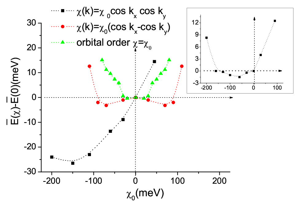
In the absence of AFM order, the results for $0.6\%$ hole-doping on a $18\times 18$ lattice using $(U_{1},U_{2},J_{H})=(4,2,0.7)$eV are shown in the main panel of Fig.1. The black and red symbols represent $\bar{E}(\chi_{0})-\bar{E}(0)$ as a function of $\chi_{0}$ with $g_{1,2}$ fixed at their optimized values. (The optimized $\left(g_{1},g_{2}\right)\approx\left(0.31(4),0.76(4)\right)$ are nearly independent of $\chi$, as the energy gain associated with their optimization is much larger than that associated with optimization of $\chi$.) From Fig. 1, it is clear that while both $\cos k_{x}\cos k_{y}$ and $\cos k_{x}-\cos k_{y}$ FS distortions gain energy, the former is the most energetically favorable one. This is consistent with the FRG prediction. The green symbols in Fig.1 represent the energy reduction due to a real space version of orbital order (see later). We note that it is not energetically favorable in the non-magnetic state. At the optimal $\chi_{0}$ the total energy gain is about $27$meV per site. The negative $\chi_{0}$ moves the bands near $\Gamma$ downward and the bands near $M$ upward. As a result it shrinks both the electron and hole pockets (it actually splits each electron pocket into two smaller ones). The distorted Fermi surface is compared with the undistorted one in Fig. 2(a,b). The above results are completely consistent with the FRG prediction[18]. In the inset of Fig. 1, we show the $\bar{E}(\chi_{0})-\bar{E}(0)$ versus $\chi_{0}$ plot for $U_{1}=2,U_{2}=1,J_{H}=0.35$ eV with $\cos k_{x}\cdot\cos k_{y}$ form-factor at 13% hole doping. The resulting relative energy shift of the bands near $\Gamma$ and $M$ is $90-126$ meV which is in good quantitative agreement with the experimentally observed $\sim 100$ meV relative shift[26, 29].

Orbital order in the AFM state The $|\psi_{MF}\rangle$ for the AFM ordered state is the ground state of the following mean-field Hamiltonian,

where $H_{0}$ is given by either Eq. 4 or Eq. 6. Here $\mathbf{Q}=\left(\pi,0\right)$ is the AFM ordering wave vector. As for $M_{\mu\nu}$ we used the mean-field result of Ref.[30] where the non-zero $M_{\mu\nu}$ are $M_{\mu\mu},\mu=1,..,5$, and $M_{15},M_{51}\left(=M_{15}\right)$. The variational study is performed by keeping the ratio between the optimal mean-field parameters ,$(M_{22},M_{33},M_{44},M_{55},M_{15})/M_{11}=(0.95,1.03,1.1,0.76,-0.096)$, while allowing $M_{11}$ to vary. For $(U_{1},U_{2},J_{H})=(4,2,0.7)$eV at 0.6% electron-doping (on $18\times 18$ lattice) we found $\left(g_{1},g_{2}\right)=\left(0.49(0),0.76(6)\right),M_{11}=1.4eV$, with a total energy reduction of about $3.0$eV per site, with nearly $2\mu_{B}$ ordering moment. This value is significantly larger than the measured ones for the stoichiometric compounds. The discrepancy can be due to the omission of the fluctuations in the orientation of magnetic moments and the ordering wavevectors , and/or the large values of the interaction parameters.

In view of the strong atomic-like ordering moments in the AFM state obtained above, when studying the orbital ordering in the magnetic state we also adopt a real space version of orbital ordering[28], where $|\psi_{MF}\rangle$ is the ground state of

Here $n_{i\alpha\sigma}=c^{\dagger}_{i\alpha\sigma}c_{i\alpha\sigma}$. We note that the orbital $d_{xz},d_{yz}$ we use are $45^{o}$ rotated from the $d_{XZ},d_{YZ}$ orbitals in Ref[15]. From Fig.3, we conclude that in the presence of AFM, the real-space $d_{xz}/d_{yz}$ orbital order is the most energetically favorable (we suspect this is due to the fact that the large, localized, ordering moment in the AFM state). It produces a total energy gain of about $4.6$meV per site. At the optimal $\chi_{0}$ the occupation-number difference between the $xz$ and $yz$ orbitals is $\bar{n}_{d_{xz}}-\bar{n}_{d_{yz}}=0.20(1).$ This value is enhanced above the $\sim 0.15$ occupation difference already present in the pure AFM state. Our result agrees qualitatively with a recent photoemission result[27] and a first principle Wannier function calculation.[28]. Comparing this result with the green symbols of Fig.1(a), we conclude that this orbital order is stabilized by the AFM.

Superconducting pairing The $\left|\psi_{MF}\right>$ we use for studying pairing is the ground state of the following mean-field Hamiltonian

We have studied four different types of gap functions:

In addition we only allow pairing in bands that cross the Fermi energy. This is an excellent approximation because, as shown below, the gaps are quite small.

Our calculations for the SC state were carried out on a $10\times 10$ lattice at $10\%$ hole doping. The optimized $\left(g_{1},g_{2}\right)\approx\left(0.31(1),0.76(2)\right)$. Again, to an excellent approximation, the optimal value of $g_{1,2}$ and $\mu_{c}$ do not depends on $\Delta_{0}$. The results for $\bar{E}(\Delta_{0})-\bar{E}(0)$ with $\left(g_{1},g_{2},\mu_{c}\right)$ fixed at their optimal values are shown in Fig. 4. The results suggest that while both conventional-$s$ and $d_{x^{2}-y^{2}}$ pairing raise the energy, $s_{\pm}$ and extended-$s$ lower it.

Interestingly, our result suggests the extended-$s$ ($\Delta_{0}\left(\cos k_{x}+\cos k_{y}\right)$) form factor is slightly favored (by $0.1\pm 0.08$ meV) over the $s_{\pm}$ ($\Delta_{0}\cos k_{x}\cdot\cos k_{y}$) one. On the surface this contradicts the predictions of $s_{\pm}$ pairing form factor! However it is important to realize that the $s_{\pm}$ gap function is not synonymous to $\cos k_{x}\cos k_{y}$. Indeed, the $s_{\pm}$ form factor obtained from several weak coupling approaches[11, 15, 14] has strong variation around the electron Fermi surfaces. We believe the near degeneracy of the extended-$s$ and the $\cos k_{x}\cos k_{y}$ form factors suggests the optimal pairing form factor is a linear combination of the two (hence is anisotropic on the electron pockets). However it is extremely computing time consuming to verify this, and we have not been able to do it. In addition, we caution that the degree of the gap function variation on the electron pockets will depends on the values of the parameters. We cannot rule out that for other parameter sets the $\cos k_{x}\cos k_{y}$ can be the leading pairing form factor. Finally, the optimal gap amplitudes for the two symmetries are about $18$meV and $20-22$meV respectively. Order of magnitude wise these values are not far from the experimentally measured gap scales.

In conclusion, we have performed variational Monte-Carlo calculation to check the validity of our previous results based on weak-coupling approximation. The results are qualitatively consistent. We caution that because of the time consuming nature of the calculation we are only able to study two sets of interaction parameters. Clearly we can not rule of the possibility that quantitative aspects of the above results will be sensitive to the precise values of the interaction parameters.

Acknowledgement: We thank Zheng-Yu Weng for sharing computer resources and Hong Yao, Ying Ran and Tao Li for helpful discussions. We acknowledge the support by the NSFC Grant No.10704008 (FY); BRYS Program of Tsinghua University and NSFC Grant No. 10944002 (HZ); and the DOE grant number DE-AC02-05CH11231 (DHL). This research also use the resources of NERSC supported by the Office of Science of the U.S. Department of Energy under Contract No. DE-AC02-05CH11231.

References

- [1] For a review and further references see P. W. Anderson, P. A. Lee, M. Randeria, T. M. Rice, N. Trivedi, and F. C. Zhang, J. Phys.: Condens. Matter 16 R755 (2004).
- [2] T.A.Maier, and D.J.Scalapino, Phys. Rev. B 78, 020514(R) (2008).
- [3] M.M. Korshunov, and I. Eremin, Phys. Rev. B 78, 140509(R) (2008).
- [4] F. Wang, H. Zhai, and D.-H. Lee, Europhys. Lett. 85, 37005 (2009).
- [5] Y.Y.Zhang, C.Fang, X. Zhou, K. Seo, W.F.Tsai, B.A. Bernevig, and J. Hu, Phys. Rev. B 80, 094528 (2009).
- [6] M. D. Lumsden et al, Phys. Rev. Lett. 102, 107005 (2009); S.Chi et al, Phys. Rev. Lett 102, 107006 (2009); S. Li et al, Phys. Rev. B 79, 174527 (2009); D. S. Inosov et al, Nature Physics 6, 178-181 (2010); J. Zhao et al, arXiv:0908.0954 (2009).
- [7] T. Hanaguri, S. Niitaka, K. Kuroki, and H. Takagi, Science 328, 474 (2010).
- [8] K.Seo, B. A. Bernevig, Jiangping Hu, Phys. Rev. Lett. 101, 206404 (2008).
- [9] I.I. Mazin, D.J. Singh, M.D. Johannes, and M.H. Du, Phys. Rev. Lett. 101, 057003 (2008).
- [10] Z.J. Yao, J.X. Li, and Z. D. Wang, New J. Phys. 11, 025009 (2009).
- [11] F. Wang, H. Zhai, Y. Ran, A. Vishwanath, and D.-H. Lee, arXiv:0805.3343 (2008);Phys. Rev. Lett. 102, 047005 (2009).
- [12] A. V. Chubukov, D. V. Efremov, and I. Eremin, Phys. Rev. B 78, 134512 (2008).
- [13] H. Ikeda, J. Phys. Soc. Jpn. 77, 123707 (2008).
- [14] S. Graser, T. A. Maier, P. J. Hirschfeld, and D. J. Scalapino, New J. Phys. 11, 025016 (2009).
- [15] K. Kuroki, S. Onari, R. Arita, H. Usui, Y. Tanaka, H. Kontani, and H. Aoki, Phys. Rev. Lett. 101, 087004 (2008).
- [16] K. Kuroki, H. Usui, S. Onari, R. Arita, and H. Aoki, Phys. Rev. B 79, 224511 (2009).
- [17] T.A. Maier, S. Graser, D.J. Scalapino, and P.J. Hirschfeld, Phys. Rev. B 79, 224510 (2009).
- [18] H. Zhai, F. Wang, and D.-H. Lee, Physical Review B, 80, 064517 (2009).
- [19] F. Wang, H. Zhai, and D.-H. Lee, Phys. Rev. B 81, 184512 (2010).
- [20] A.V. Chubukov, M.G. Vavilov, and A.B. Vorontsov, Phys. Rev. B 80, 140515(R) (2009); R. Thomale, C. Platt, J. Hu, C. Honerkamp, and B. A. Bernevig, Phys. Rev. B 80, 180505(R) (2009).
- [21] W.L. Yang et al, Phys. Rev. B 80, 014508 (2009)
- [22] See, e.g., M. M. Qazilbash, J. J. Hamlin, R. E. Baumbach, Lijun Zhang, D. J. Singh, M. B. Maple, D. N. Basov Nature Physics 5, 647 (2009).
- [23] L. Craco et al, Phys. Rev. B 78, 134511 (2008); K. Haule et al, Phys. Rev. Lett. 100, 226402 (2008).
- [24] Some other LDA+DMFT studies listed below provide a different picture for the model parameter. Namely, that U 4 is relevant for a model including the As p-orbitals, but that a reduced U should be used in the 5-band model. V. I. Anisimov, Dm. M. Korotin, M. A. Korotin, A. V. Kozhevnikov, J. Kunes, A. O. Shorikov, S. L. Skornyakov, S. V. Streltsov, J. Phys.: Condens. Matter 21 No 7, 075602(2009); M. Aichhorn, L. Pourovskii, V. Vildosola, M. Ferrero, O. Parcollet, T. Miyake, A. Georges, and S. Biermann, Phys. Rev. B 80, 085101(2009).
- [25] D. Ceperley, G. V. Chester, and K. H. Kalos, Phys. Rev. B 16, 3081 (1977); C. J. Umrigar, K. G. Wilson, and J. W. Wilkins, Phys. Rev. Lett. 60, 1719 (1988).
- [26] Donghui Lu, private communication.
- [27] M. Yi, et al, arXiv 1011,0050.
- [28] Chi-Cheng Lee, Wei-Guo Yin, and Wei Ku, Phys. Rev. Lett. 103, 267001 (2009)
- [29] A.I. Coldea, J.D. Fletcher, A. Carrington, J.G. Analytis, A.F. Bangura, J.-H. Chu, A.S. Erickson, I.R. Fisher, N.E. Hussey, R.D. McDonald, Phys. Rev. Lett. 101, 216402 (2008).
- [30] Ying Ran, Fa Wang, Hui Zhai, Ashvin Vishwanath, Dung-Hai Lee, Phys. Rev. B 79, 014505 (2009)
- [31] J.D. Fletcher, A. Serafin, L. Malone, J. Analytis, J-H Chu, A.S. Erickson, I.R. Fisher, and A. Carrington, Phys. Rev. Lett. 102, 147001 (2009).
- [32] C. W. Hicks, T. M. Lippman, M. E. Huber, J. G. Analytis, J. H. Chu, A. S. Erickson, I. R. Fisher, and K. A. Moler, Phys. Rev. Lett. 103, 127003 (2009).