IPMU10-0113
ICRR-Report-570-2010-3
Gluon contribution to the dark matter direct detection
Junji Hisanoa,b, Koji Ishiwatac, and Natsumi Nagataa,d,
aDepartment of Physics, Nagoya University, Nagoya 464-8602, Japan
bInstitute for the Physics and Mathematics of the Universe,
University of Tokyo, Kashiwa 277-8568, Japan
cInstitute for Cosmic Ray Research, University of Tokyo,
Kashiwa 277-8582, Japan
dDepartment of Physics, University of Tokyo, Tokyo 113-0033, Japan
In this article we have calculated the spin-independent cross section of nucleon-dark matter scattering process at loop level, which is relevant to dark matter direct detection. Paying particular attention to the scattering of gluon with dark matter, which contributes as leading order in the perturbation, we have systematically evaluated loop diagrams with tracking the characteristic loop momentum which dominates in the loops. Here loop diagrams whose typical loop momentum scales are the masses of quarks and other heavier particles are separately presented. Then, we have properly taken into account each contribution to give the cross section. We assume that the dark matter is pure bino or wino in the supersymmetric models. The application to other models is straightforward.
1 Introduction
The existence of nonbaryonic dark matter has been established by cosmological observations [1]. Weakly-interacting massive particles (WIMPs) are attractive candidates for dark matter, and many models are proposed to predict WIMPs. The lightest neutralino in the minimal supersymmetric standard model (MSSM) has been extensively studied among them.
The direct detection experiments of WIMP dark matter are one of the methods for probing the nature of the dark matter. In the experiments, one searches for the signatures of WIMP-nucleon scattering. Many experiments have searched for the dark matter signals, and their sensitivities have been improved. The CDMS II experiment reported the final result for the five-tower WIMP search last year [2]. They observed two events in the dark matter signal region for the detector; their data set the upper limit on the spin-independent WIMP-nucleon elastic scattering cross section (donated as ) of cm2 for a WIMP of mass 70 GeV. This year the XENON100 experiment also started, and has already reported the first result [3]; they have given the upper limit as cm2 for WIMPs of mass 55 GeV. In addition, the XMASS experiment will start soon [4]. Prospects for sensitivities of these new experiments are around cm2, and they cover broad parameter space of the neutralino dark matter scenario in the MSSM.
In order to study the nature of dark matter based on those latest experiments, we need to evaluate the WIMP-nucleon elastic scattering cross section precisely. The WIMP-nucleon elastic scattering is induced by effective interactions of the WIMP with quarks or gluon at parton level. The effective interaction with the gluon is typically of higher order of the QCD coupling constant than those with quarks in many models, since the WIMP interacts with the gluon via loop diagrams including quarks and/or other colored particles. However, the effective scalar interaction with the gluon may make the leading contribution in the spin-independent (SI) cross section. This comes from the fact that the nucleon mass is dominated by gluon contribution.
The effective interaction of the WIMP with the gluon is generated by loop diagrams. The loop momentum which dominates the integration is characterized by the mass scale of either heavy particles (such as WIMP mass) or quarks. We call the former (the latter) the “short-distance” (“long-distance”) contribution. The long-distance contribution to the effective scalar operator of the WIMP with gluon is approximately evaluated from the effective scalar operators with quarks by using the trace anomaly of QCD. On the other hand, the short-distance contribution needs to be explicitly calculated. Drees and Nojiri calculated the one-loop box diagrams for gluon-neutralino scattering in the MSSM, and included the short-distance contribution to the SI cross section [5]. Although the SI cross section is evaluated in various models, the short-distance contribution is not included in many papers.
In this paper we show a method to include the short- and long-distance contributions to the SI cross section systematically. We use the Fock-Schwinger gauge for the gluon field. This is frequently used in the QCD sum rules in order to evaluate the operator product expansions [6]. It is found that this gauge makes the calculation for the gluon contribution to the SI cross section much more transparent. In addition, we separately calculate short- and long-distance contributions, which makes it possible to add each contribution properly to the cross section.
So as to study the details of gluon-neutralino scattering, we consider two cases where the lightest neutralino is pure bino and wino in the framework of the MSSM. For the bino-like neutralino case, the neutralino-quark scattering is induced by squark exchange at tree-level, and the neutralino-gluon scattering is generated at one-loop level. Calculating all the relevant diagrams at leading order, consequently we have found that the long-distance contribution of light quarks is partially regarded as the short-distance one in the calculation as Ref. [5]. This correction changes the SI cross section slightly in the MSSM. On the other hand, for the wino-like neutralino case, when superparticles except for the gauginos and the heavier Higgs bosons are decoupled in the MSSM, the neutralino-nucleon scattering process is dominated by weak gauge boson loop diagrams [7]. We evaluated the effective interactions of the neutralino with quarks at one-loop level and those with gluon at two-loop level. Here we use the Fock-Schwinger gauge for the gluon field, again; the result has been published in Ref. [8]. In this paper, we show detail of the evaluation.
Our method to evaluate the effective interaction of the WIMP with the gluon is applicable to other models of dark matter, such as universal extra-dimension scenario. Such analysis will be given elsewhere [9].
This article is organized as follows. In Sec. 2 we summarize the effective couplings of the WIMP with quarks and the gluon. We assume that the WIMP is Majorana fermion. Here we explain how to evaluate the effective interaction of the WIMP with the gluon. In Sec. 3, assuming that the neutralino is bino-like, we evaluate the effective couplings of the neutralino with quarks and the gluon by using the Fock-Schwinger gauge for the gluon field. Then we consider the case that the neutralino is wino-like where the neutralino-nucleon scattering is generated at loop-diagrams due to the weak interaction in Sec. 4. Finally Sec. 5 is devoted to the conclusion. In the Appendix, we show the propagators of scalar and fermion in a gluon background (Fock-Schwinger gauge) and other useful formulas for evaluation of effective interaction of the WIMP with the gluon.
2 Effective interaction for WIMP-nucleon scattering
First, we summarize the effective interactions of the WIMP with light quarks () and gluon, which are relevant to the WIMP-nucleon spin-independent scattering. They are given as follows,
| (1) |
where
| (2) | |||||
| (3) |
is the WIMP which we assume to be Majorana fermion as it is mentioned in the Introduction. and are masses for the WIMP and quarks, respectively. The second and third terms in and depend on the twist-2 operators (traceless parts of the energy-momentum tensor) for quarks and gluon, respectively,
| (4) |
Here the covariant derivative is defined as (, and are the coupling constant and generator, and the gluon field, respectively), and is the field strength tensor of gluon.
The SI cross section of the WIMP with target nuclei is expressed compactly in terms of the SI coupling of the neutralino with nucleon [10];
| (5) |
where is the mass of target nucleus, and and are proton and neutron numbers in the target nucleus, respectively. The SI coupling of the neutralino with nucleon is given by the coefficients and matrix elements of the effective operators in and as11 1 We have included contributions from effective interactions with twist-2 operators for charm and bottom quarks, and , in Eq. (6). See later discussion.
| (6) | |||||
The matrix elements of the effective operators are expressed by using nucleon mass as
| (7) |
In the matrix elements of twist-2 operators, , and are the second moments of the parton distribution functions (PDFs) of quark, antiquark and gluon, respectively,
| (8) | |||||
| (9) |
For the numerical calculation, we describe the input parameters for the hadronic matrix elements that we use in this article. The mass fractions of light quarks, , are expressed as [11]
| (10) |
for proton/neutron. Here,
| (11) |
The recent lattice simulation predicts that and [12]. Combined with [11, 13], we get = 0.023, = 0.032, and =0.020 for the proton, and =0.017, = 0.041, and = 0.020 for the neutron. In our numerical evaluation, we use the center value for each parameters.
The second moments of the PDFs of quark, antiquark and gluon are scale-dependent, and are mixed with each other once the QCD radiative corrections are included. Thus, the coefficients of the terms with twist-2 operators become scale-independent after they are multiplied by the second moments of the PDFs [5]. We use the second moments for the PDFs at the scale of boson mass, and include bottom and charm quark contributions, as given in Eq. (6). The second moments are evaluated from the CTEQ parton distribution [14] as
| (12) |
for the proton. Those for the neutron are given by an exchange of up and down quarks.
For the calculation of at leading order, we give some remarks. The effective interactions of the WIMP with the gluon are of higher order of than those of the light quarks in many models including the MSSM. However, it is found in Eq. (6) that the effective scalar coupling of the WIMP with the gluon gives the leading contribution to the cross section even if it is suppressed by one-loop factor compared with those of light quarks. On the other hand, the contributions with the twist-2 operators of the gluon are of the next-leading as and are suppressed by . Then, we ignore them in this paper.
Finally we explain the evaluation of . In general, the effective coupling of - scattering is induced by loop diagrams in which virtual quarks and other heavy particles run (like squarks in the MSSM). Consequently, the integral momentum around not only the quark mass scale but also the heavy particle one contributes. (As we described in the Introduction, we call them as “long-” and “short-distance” contributions, respectively.) Thus, in order to take into account both contributions accurately for general cases, we must calculate loop diagrams explicitly. So as to calculate diagrams including the quark systematically, we separate the two contributions as
| (13) |
In the long-distance contribution, there is another approximated way to evaluate the heavy quark contribution, which is valid in the limit of large mass of heavy particles. After integrating out heavier particles than heavy quarks, we write down the effective Lagrangian for heavy quarks: 22 2 We used the equation of motion for the quark to reduce the effective Lagrangian. Though the heavy quarks are in loops in the evaluation of the effective interaction of the WIMP with the gluon, it is justified to use it. See Ref. [15] and references in it. We also explicitly checked that the effective interaction leads to the same result for as . . We calculate one-loop triangle diagrams in which heavy quarks rotate to emit two gluons, and get33 3 This result is also obtained in another way. It is pointed out in Ref. [5] that the effective interactions which come from heavy quark loops are approximately calculated in the effective interaction of the WIMP with heavy quarks, using the trace anomaly of energy-momentum tensor in QCD [16]. When the virtual heavy quark is the only particle in the loop diagram, the integrated-out heavy quark converts to the gluon operator as , which gives the same result as Eq. (14).
| (14) |
(See Appendix for detail.) Thus, we expect that
| (15) |
in the limit of the large mass of heavy particles. (This can be utilized to check explicit loop calculation. See the following sections.) In the explicit loop calculation, we observe that the momentum with the scale of quark mass dominates the integral to give a factor (which is canceled in ).
For light quark contributions in long-distance loops, on the contrary, we must not include them in the same manner as heavy quark ones when we evaluate . As we saw in the above calculation, the loop momentum is dominated by quark mass; thus, the propagators for the soft quark whose momentum and mass are smaller than the QCD scale are determined entirely by confinement dynamics. The corresponding effect should be included in the matrix element [6]. That is why the light quark loops must not be counted in the evaluation of .
Being aware of this fact, we sum up for quarks properly and get
| (16) |
In addition, it is pointed out [17] that the long-distance contributions to suffer from large QCD correction. The corrections to Eq. (14) are given as
| (17) |
where . We take and for ( is boson mass), and in our numerical calculation. Then, rewriting Eq. (16) with the QCD correction, we finally get
| (18) |
In the case where the WIMP interacts with the Higgs boson, the short-distance contribution to the effective interaction of the WIMP with the gluon is not generated at the leading order. Then, we can easily evaluate the SI cross section without explicit calculation of loop diagrams by using Eq. (17). However, it is not the case for the bino-like neutralino dark matter. In the next section, we consider the case where the lightest neutralino is almost pure bino in the MSSM. The bino interacts with quarks and squarks. We will see that the squark-quark loop diagrams give both short- and long-distance contributions.
3 Bino-like neutralino dark matter
The lightest neutralino interacts with quarks and gluon in diagrams with Higgs boson exchange or squark exchange. When the Higgsino-gaugino mixing is not negligible, the Higgs boson exchange tends to dominate in the SI - scattering. On the other hand, when the mixing is negligible and squark masses are comparable to the neutralino mass, the squark exchange dominates over the Higgs boson exchange. In this section, we take a limit ( is the Higgsino mass parameter in superpotential) and consider the case where the lightest neutralino is almost pure bino. The extension to the general cases is straightforward.
Before going to the numerical calculation, we show the couplings of the effective Lagrangian which are given by the explicit calculation of tree- and loop-level scattering amplitudes. The following calculation is applicable to the models in which the WIMP interacts with quarks and new colored scalars. (For the time being, we do not distinguish a light or heavy quark for “” unless it is expressly described, and provide the analytic results of the effective couplings.)
First, we simply parametrize the neutralino interaction with quark and squark as
| (19) |
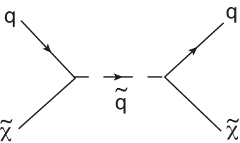
Integrating out squarks at tree level (the corresponding diagram is shown in Fig. 1), the effective interaction with light quarks in Eq. (2) is generated as
| (20) |
Here we take the zero quark mass limit.
At loop level, the interactions of the WIMP with gluon are generated. The leading contribution is from one-loop diagrams including each heavy or light quark in Fig. 2. For the calculation of these diagrams, we adopt the Fock-Schwinger gauge for the gluon field:
| (21) |
By using this gauge, we can express the gauge field by the field strength tensor as
| (22) |
so that we can extract out relevant effective interaction of the gluon easily. On the other hand, since the translation invariance is lost in this gauge, we have to distinguish two propagators for quarks in a gluon background,
| (23) |
and those for squarks,
| (24) |
In the Appendix, propagators of the colored fermion and boson in the Fock-Schwinger gauge are collected for convenience.
The two-point function of the neutralino in the gluon background (donated as ) is calculated by using the above propagators; then the effective scalar coupling of neutralino and gluon is derived from the two-point function as
| (25) |
where
| (26) | |||||
Here, the factor comes from the neutralino being Majorana and “” means to extract the coefficient for terms proportional to . For simplicity, we write to which the single flavor of quark (and squark) contributes. As we described in the previous section, we decompose it into short- and long-distance contributions and write as
| (27) |

The short-distance contribution comes from diagram (b) in Fig. 2, while the long-distance one is from diagram (d). The diagrams (a) and (c) vanish in our gauge. (See Appendix.) The mass functions are given as
| (28) |
where
| (29) |
In the above expression, it is apparent that the typical momentum scale of integral is dominated by the squark mass in the short-distance contribution while it is dominated by quark mass in the long-distance one. With straightforward calculation of the integral, we have finally obtained
Here,
When we take zero quark mass limit, the mass functions are approximated as
| (34) |
For the heavy quark loop in the long-distance contribution, it is checked that Eq. (15) is satisfied from Eqs. (14) and (20), just replacing as , when , as expected. The mass function in the long-distance contribution is not singular in a limit of zero quark mass, while is. This is because is proportional to before the loop momentum integral and the loop momentum integral leads to .
With all results, we obtain the effective coupling of the neutralino with gluon. As we described in the previous section, the contribution of light quarks should not be included in since the loop momentum has infrared cutoff, GeV, implicitly. In Ref. [5], however, the long-distance contribution of light quarks, i.e. , is added in . This point can be seen by comparing our result with theirs in a simple expression under a certain limit. In the case of , for instance, our result gives
| (35) |
Focusing on the term which is proportional to for the comparison, the result given in Ref. [5] has the form in which the term, , is added to the above expression. We found that the long-distance contribution of light quarks, proportional to , is regarded as the short-distance one in Ref. [5] and added in .

Now we numerically show the cross section for the SI scattering of the bino-like neutralino with nucleon. The interaction of the bino-like neutralino with quark and squark is given as
| (36) |
where and is the gauge coupling constant of . and are the lighter and heavier squark, respectively, and the coefficients, and , are
| (37) |
where , and . The mixing angle of squark mass matrix is
| (38) |
where we parametrize mass terms of left-handed and right-handed squark ( and ) as
| (39) |
From the interaction Lagrangian, and can be written as
| (40) |
Then, we numerically calculate the SI cross section, using Eqs. (18) and (20). (Here we include the QCD correction to the long-distance contribution to .)
The cross section for SI scattering with proton, , is plotted in Fig. 3 as a function of the neutralino mass. Here we give several results in the figure by taking , , = (1.5, 1.2, 0.1), (2.0, 1.5, 1.0), and (3.0, 2.0, 1.0) from top to bottom in solid lines. It is found that the cross section is suppressed as the neutralino mass become larger, and so it is unless masses of the neutralino and squarks are degenerate. In Fig. 4, we present tree- and loop-level contributions to SI coupling in solid and dashed lines, respectively. The tree-level contribution, which mainly comes from in Eq. (20), is dominant, and the quark-squark loop contribution is subdominant; it accounts for % in the SI cross section. Just for reference, we also give the contribution from loop diagram in the case where the light quark contribution of long-distance is added in (dashed-dot lines in Figs. 3 and 4). We have seen that the difference between our evaluation and the reference one is %. As shown in Fig. 3, the result is almost independent of the choice of the squark masses if they are in the same order of bino mass. This is because both and give the same order of contribution to in such a case.44 4 We note that there exist benchmark points to explain the observed dark matter abundance in which squark masses are much larger than the bino one. In such a case, the lightest neutralino should be a mixed state of bino and Higgsinos so that the SI cross section is determined by the Higgs boson exchange. We have checked that the long-distance contribution induced by the Higgs exchange is correctly evaluated in the previous works (e.g. Ref. [5]) and the numerical result of the cross section in such a case is unchanged. The result, which has improved theoretical calculation of the SI cross section of dark matter with nucleon, will be important when we determine the local density and/or cross section of dark matter in the future experiments. Finally we also note that, in the public codes for studies of the neutralino dark matter, DarkSUSY [18] and MicroOMEGA [19], the gluon contribution to the spin-independent cross section is included by following Ref. [5]. Those programs should be corrected when one needs to calculate the cross section at less than % error.

4 Wino-like neutralino dark matter
In the anomaly mediation [20] the wino-like neutralino is a candidate for dark matter in the universe. The thermal relic abundance of the wino-like neutralino in the Universe is consistent with the WMAP observation when the wino mass is from 2.7 TeV to 3.0 TeV [21]. The lighter wino-like neutralino may be consistent with the observation of the dark matter abundance in the Universe if decay of gravitino or other quasistable particles may produce the dark matter nonthermally [22, 23].
The tree-level contribution to the cross section for elastic scattering of the wino-like neutralino with nucleon is evaluated in Ref. [24]. However, in the case that the superparticles except for gauginos and the heavier Higgs bosons are much heavier than the weak scale in the MSSM, the tree-level interactions of the neutralino to quarks are quite suppressed. The scattering process is dominated by the boson loop diagrams. Recently, we reevaluated the cross section for SI scattering of the wino-like neutralino with nucleon [8]. In the work, the two-loop contribution to the effective interaction of the neutralino with gluon is included, in addition to one-loop ones to the interaction with quarks. Then it is confirmed that both one- and two-loop contributions act as the leading contribution in the SI scattering process. Although calculation of two-loop diagrams is much involved, it can be dealt with systematically in the Fock-Schwinger gauge. In the following, we show the technical detail of the calculation.
Winos are gauginos which are partners of the gauge bosons in the MSSM, and they have the weak interaction. The relevant operators in our discussion is
| (41) |
where is the gauge coupling constant of . The wino-like neutralino accompanies the wino-like chargino (). The mass difference is dominated by one-loop contribution unless the Higgsino and wino masses are almost degenerate.
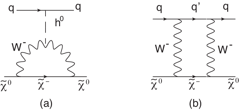
Before getting down to the two-loop calculation, we quickly review one-loop contribution to the SI interaction of -. The effective interactions of with light quarks in the effective Lagrangian are generated by diagrams in Fig. 5. The diagram (a), which is induced by the standard-model Higgs boson () exchange, contributes to , while the diagram (b) generates the other terms in the effective Lagrangian. The results are given in Ref. [8]. The obtained effective couplings are finite in the limit . Thus, the SI interaction of - is not suppressed even if the wino-like neutralino is much larger than the boson mass, as pointed out in Ref. [7].
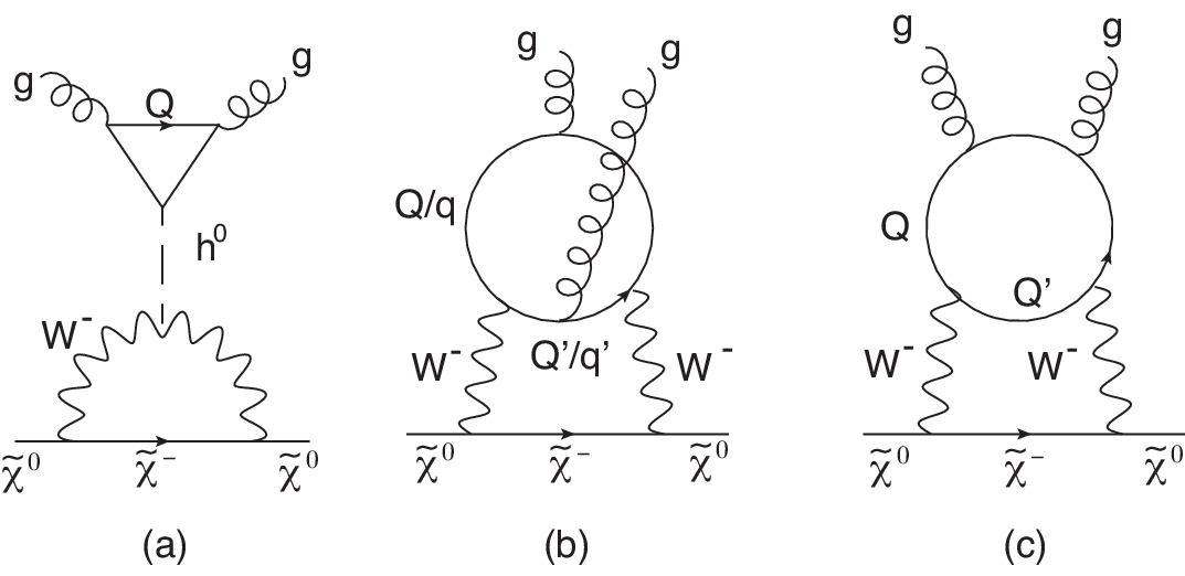
Next, let us derive the effective interaction of the neutralino with gluon, which is generated at two-loop level. Three types of diagrams in Fig. 6 contribute to . Diagram (a) includes heavy quark loops, and it is evaluated from as given in Eq. (17). On the other hand, we need to calculate irreducible two-loop diagrams (b) and (c) explicitly. In order to handle this calculation, it is convenient to evaluate the vacuum polarization tensor of boson in the gluon background,
| (42) |
Here, and are propagators of up-type and down-type quarks, respectively, in the Fock-Schwinger gauge for gluon field. The vacuum polarization tensor is decomposed to the transverse and longitudinal parts as
| (43) |
We found from an explicit calculation that the longitudinal part of the self energy does not contribute to . Thus, what we have to calculate is coefficients for terms with gluon scalar operator in , i.e. .
For the calculation , we furthermore decompose the contributions from diagram (b) and (c) in Fig. 6 as follows;
| (44) |
where is the flavor index and . is obtained from diagram (b) and () is from diagram (c) in which gluon lines are attached with the propagator of up- (down-) type quark. In the above expressions, loop integrals are defined as
| (45) |
where and are masses of up-type and down-type quarks, respectively.
Notice that, in the loop integrals for the self-energy part of diagram (c), the typical momentum is the mass of quark which emit two gluons, i.e. the up- and down-type quark mass in and , respectively. This fact means that diagram (c) gives the long-distance contribution in the part of one-loop self-energy of the boson. Therefore, we add the contribution of for and 3 (up-type quark is heavy one) and for (down-type quark is heavy one). On the other hand, the loop momentum of quark loop in diagram (b) is dominated by the external momentum of the quark loop diagram; therefore, all quarks contribute in the loop. Then is properly obtained as
| (46) |
Executing the integral and neglecting quark masses except for the top one, we finally get
| (47) |
The first term in the right-handed side comes from loops of the third generation, while the second term is induced by the first- and second-generation quarks. We observed that the singular terms in are cancelled in the loop integrals of so that vanishes in the limit. Actually, this is expected from the indication of Eq. (15) and the fact that diagram (b) in Fig. 5 does not contribute to the neutralino-quark scalar coupling in a limit of zero quark mass [8].
Combining the above results, we get as
| (48) |
where and are the Higgs and -boson masses, respectively, and . In addition, we include the QCD correction to the long-distance contribution of heavy quarks to . The mass functions , and are given in Ref. [7].

In Fig. 7, we show the numerical result for the SI cross section. Here the evaluation with (without) the QCD correction is given by taking , , and . While the latter two values may not be realistic in the MSSM, the next-minimal supersymmetric standard model, for example, may predict a larger Higgs boson mass. It is found from the figure that the cross section is more suppressed unless the Higgs boson mass is larger than a few hundred GeV. This fact is the consequence of an accidental cancellation in SI coupling as it is shown in Ref. [8]; the QCD correction makes the contribution from the Higgs boson exchange larger so that the cancellation works hard.55 5 In Ref. [8], the QCD correction for long-distance contribution and the contribution from the twist-2 operators of bottom and charm quarks are not included. On the other hand, the effect of the cancellation becomes weaker as the Higgs boson mass is larger.
5 Conclusion
In this article, we have systematically calculated the spin-independent cross section of the nucleon-lightest neutralino scattering process at loop level. Although the one-loop (higher-loop) diagrams are usually the higher-order of quantum correction to tree-level (one-loop) ones, such higher order diagrams of neutralino-gluon scattering work as the leading contribution. We have evaluated the effective coupling of neutralino-gluon scattering by explicit calculation of loop diagrams in the Fock-Schwinger gauge. In this gauge, we can calculate systematically the loop diagrams, tracking the loop momentum scales which dominate in the integrals. Making the most of it, we have separately evaluated short- and long-distance contributions in the loop diagrams, i.e. the contributions in which the loop momentum is characterized by masses of new particles heavier than quarks (like mass scale of neutralino or squark) and those of quarks. Being aware that the contribution of light quarks must not be included in the long-distance diagrams, we have numerically calculated the spin-independent effective coupling to give the cross section of nucleon-neutralino scattering. In order to focus on the contribution of neutralino-gluon scattering, we considered the bino- and wino-like neutralino cases. In the former case, we have found that the effective coupling of neutralino-gluon scattering differs by 20-30 % from the one evaluated in the case where light quarks are included in the long-distance contribution incorrectly; it gives alteration in the SI cross section. This improvement in the theoretical calculation of the cross section will be essential when we explore the nature (i.e. interaction and/or local density) of dark matter in the future experiments. On the other hand, in the latter case, the quark- and gluon-neutralino scattering contributes in almost the same magnitude and opposite sign. Then, they cancel each other to suppress the SI cross section. Here we have also taken into account QCD correction for long-distance contribution; consequently, we have found that the cancellation works hard.
Acknowledgment
The work was supported in part by the Grant-in-Aid for the Ministry of Education, Culture, Sports, Science, and Technology, Government of Japan, No. 20244037, No. 2054252 and No. 2244021 (J.H.) and Research Fellowships of the Japan Society for the Promotion of Science for Young Scientists (K.I.). The work of J.H. is also supported by the World Premier International Research Center Initiative (WPI Initiative), MEXT, Japan.
Appendix A Propagators in Fock-Schwinger gauge
Here we present colored fermion and scalar boson propagators in the Fock-Schwinger gauge for gluon, and useful formulas to evaluate effective coupling of WIMP and gluon. We also show derivation of the coupling in a model in which the WIMP has an interaction with the Higgs boson, as a simple exercise.
Defining gluon field in covariant derivative, , the gauge-fixing condition in the Fock-Schwinger gauge is written as
| (49) |
In this gauge, the vector field can be directly expressed in the terms of the gluon field strength tensor as
While the gauge-fixing condition breaks the translation invariance, it is recovered in the gauge-invariant objects. The propagators of colored fermion in the gluon background are given as

| (51) | |||||
| (52) | |||||
where and . In the actual calculation, terms including covariant derivatives, such as and , are ignored, since they are irrelevant to evaluation of the SI cross section. In text we evaluate the scalar coupling of WIMP with gluon, , by extracting out the bilinear term of the gluon field strength from the WIMP ( boson) two-point function in the bino- (wino-)like neutralino dark matter case. The scalar operator of gluon is projected out from the bilinear term of the gluon field strength as
| (53) | |||||
where is the twist-2 operator of gluon (Eq. (4)) and is a higher-twist operator,
| (54) | |||||
We also give colored scalar propagators:
| (55) | |||||
| (56) | |||||

where . The scalar propagators are reduced in a more convenient form for practical usage as
| (57) | |||||
| (58) | |||||
In the calculation of the SI cross section of the bino-like neutralino in Sec. 3, the diagrams (a) and (c) in Fig. 2 are found to be zero in the Fock-Schwinger gauge, since terms except the first and fifth terms in and vanish in the calculation.
Last, we show the loop diagram calculation in the Fock-Schwinger gauge for a simple scenario as an exercise. We consider a model in which the WIMP interacts with the standard-model Higgs boson;
| (59) |
Effective interactions of with light (and heavy) quarks generated by diagram (a) in Fig. 10;
| (60) |
at leading order. Other coefficients in Eqs. (2) and (3) are zero at the leading order. The effective coupling of WIMP with gluon is induced by diagram (b) in Fig. 10;
| (61) | |||||
Here we neglected the QCD correction just for simplicity.

References
- [1] J. Dunkley et al. [WMAP Collaboration], Astrophys. J. Suppl. 180 (2009) 306.
- [2] Z. Ahmed et al. [The CDMS-II Collaboration], arXiv:0912.3592 [astro-ph.CO].
- [3] E. Aprile et al. [XENON100 Collaboration], arXiv:1005.0380 [astro-ph.CO].
- [4] H. Sekiya, for the XMASS Collaboration, arXiv:1006.1473 [astro-ph.IM].
- [5] M. Drees and M. Nojiri, Phys. Rev. D 48 (1993) 3483.
- [6] V. A. Novikov, M. A. Shifman, A. I. Vainshtein and V. I. Zakharov, Fortsch. Phys. 32 (1984) 585.
- [7] J. Hisano, S. Matsumoto, M. M. Nojiri and O. Saito, Phys. Rev. D 71 (2005) 015007.
- [8] J. Hisano, K. Ishiwata and N. Nagata, Phys. Lett. B 690 (2010) 311.
- [9] J. Hisano, K. Ishiwata, N. Nagata, and M. Yamanaka, in preparation.
- [10] G. Jungman, M. Kamionkowski and K. Griest, Phys. Rept. 267 (1996) 195.
- [11] A. Corsetti and P. Nath, Phys. Rev. D 64 (2001) 125010.
- [12] H. Ohki et al., Phys. Rev. D 78 (2008) 054502.
- [13] H. Y. Cheng, Phys. Lett. B 219 (1989) 347.
- [14] J. Pumplin, D. R. Stump, J. Huston, H. L. Lai, P. Nadolsky and W. K. Tung, JHEP 0207 (2002) 012.
- [15] W. Skiba, arXiv:1006.2142 [hep-ph].
- [16] M. A. Shifman, A. I. Vainshtein and V. I. Zakharov, Phys. Lett. B 78 (1978) 443.
- [17] A. Djouadi and M. Drees, Phys. Lett. B 484 (2000) 183.
- [18] P. Gondolo, J. Edsj, P. Ullio, L. Bergstrom, M. Schelke and E.A. Baltz, JCAP 0407 (2004) 008 [astro-ph/0406204]; See the manual ( http://www.physto.se/%7Eedsjo/darksusy/docs/Manual.pdf).
- [19] G. Belanger, F. Boudjema, A. Pukhov and A. Semenov, Comput. Phys. Commun. 180 (2009) 747 [arXiv:0803.2360 [hep-ph]].
- [20] L. Randall and R. Sundrum, Nucl. Phys. B 557 (1999) 79; G. F. Giudice, M. A. Luty, H. Murayama and R. Rattazzi, JHEP 9812 (1998) 027.
- [21] J. Hisano, S. Matsumoto, M. Nagai, O. Saito and M. Senami, Phys. Lett. B 646 (2007) 34.
- [22] T. Gherghetta, G. F. Giudice and J. D. Wells, Nucl. Phys. B 559 (1999) 27.
- [23] T. Moroi and L. Randall, Nucl. Phys. B 570 (2000) 455.
- [24] B. Murakami and J. D. Wells, Phys. Rev. D 64 (2001) 015001.