Amplification of Curvature Perturbations in Cyclic Cosmology
Abstract
We analytically and numerically show that through the cycles with nonsingular bounce the amplitude of curvature perturbation on large scale will be amplified and the power spectrum will be redden. In some sense, this amplification will eventually destroy the homogeneity of background, which will lead to the ultimate end of cycles of global universe. We argue that for the model with increasing cycles, it might be possible that a fissiparous multiverse will emerge after one or several cycles, in which the cycles will continue only at corresponding local regions.
Recently, a cosmological cyclic scenario, in which the universe experiences the periodic sequence of contractions and expansions [1], has been rewaked [2], and brought the distinct insights into the origin of observable universe. There have been lots of studies on cyclic or oscillating universe models [3],[4],[5],[6],[7],[8],[9],[10], [11],[12],[13], also [14] for a review. In general, it is thought that the background of cyclic universe is homogeneous cycle by cycle all along. However, it has been noticed that in the contracting phase the amplitude of curvature perturbation on super Hubble scale is increased, while is nearly constant in the expanding phase. Thus the net result is that the amplitude of perturbation is amplified, which seems to go along cycle by cycle [15].
Whether this amplification of perturbation actually occurs is interesting, since it will lead the global configuration of cyclic universe unexpected colorful [16]. In this paper, we will analytically and numerically show the change of power spectrum of curvature perturbation through one or several cycles. We will simulate the effect of the increasing of its amplitude on the global configuration of cyclic universe, which might dramatically alter our conventional perspective for cyclic universe.
We begin with the cyclic universe models in Fig.1, in which the nonsingular bounce is implemented by introducing a field with negative energy, which is minimally coupled to gravity. During the expansion and contraction, the universe is dominated by a normal scalar field, which oscillates in a quadratic potential and offers matter-dominated background. With the shrinking of the scale factor, the ghost field becomes dominated and finally leads the bounce take place. In the inset of Fig.1, the corresponding state parameters of models are plotted. It can be found that, due to the oscillation of the dominated scalar field, is oscillating with [17], which is matter-liked, during the contraction and expansion. While near the bounce, crosses in a very short time.

In general, the introduction of field with negative energy is only the approximative simulation of a fundamental theory below certain physical cutoff. Pointed by [18], for a ghost with a minimal coupling to gravity, as same case in our paper, the cutoff is constrained by observations of the diffuse gamma ray background with . Therefore, we can estimate the validity of our model by consider the valid physical momentum space of perturbation. Given by the cutoff , the upper limit of the comoving wave numbers is where is in units of , an adjustable parameter that can be determined by fit the time of expansion, which is , see Fig.1, to the age of observable universe, . When we use the present Hubble rate, , we can find that, during the bouncing, the upper limit of the perturbations’ comoving wave numbers is which is much larger than the largest wave number, , which is chose in following figures’, discussed in this paper. In this sense, the validity of the background model used in this paper is well guaranteed. However, one should remember that the appearance of phantom field is only an artificial approximation. Recently, the nonsingular bounce has been obtained in nonlocal higher derivative theories of gravity [19],[20], which can be ghostfree.
The primordial perturbation generated during the contraction with is scale invariant [21],[22],[23]. There also are some studies how the perturbations go through such a nonsingular bounce [24],[25],[26],[27]. The cycle plotted as the blue line is increased, because there is an inflationary epoch after the bounce in each cycle, the corresponding observable signals have been studied in e.g. [28],[29],[30]. The models with increasing cycle can be also obtained in e.g. [3],[4],[11],[12], in which the entropy is increased. However, the results of change of power spectrum of curvature perturbation through cycles are not altered qualitatively by how the increasing cycle is implemented. The examples in Fig.1 will only serve the purpose of numerical simulations in the following.
We will regard the turnaround time as the beginning of a cycle, which can be denotes as of the cycle. In each cycle the universe will orderly experience the contraction, bounce, and expansion, and then arrive at the turnaround, which signals the end of a cycle. The beginning and the end of each phase of the cycle can be denoted as , , , , and the bounce is .
The evolution of curvature perturbation under this cyclic background can be simply showed as follows. The motive equation of the curvature perturbation in the momentum space is
| (1) |
where [31],[32], and [33] for details, the prime denotes the derivative for the conformal time and . When , i.e. the perturbations are deep inside the Hubble radius, it is obviously that will oscillate with a constant amplitude. When , i.e. the perturbations are on super Hubble scale, Eq.(1) has general solution , which gives , e.g.[33], where and are constant for fixed . In general, for the contraction phase , can be obtained. Thus during the contraction with , as , the amplitude of will be dominated by term,
| (2) |
since , which is increased on large scale.
While for the expanding phase , can be obtained, where the plus is for and the minus for . In these both cases the term is decreasing. Thus the term dominates , which is constant for fixed . This means that for a cycle of cyclic universe during the contraction is increased on super horizon scale, up to the end of contracting phase in corresponding cycle, while during the expansion it becomes constant. Thus the net result is that on large scale is amplified, which is inevitable.

The spectrum index of obtained by Eq.(1) is , e.g.[34], which is scale invariant for , i.e. inflation, and for , i.e. the contraction with [21],[22],[23]. During the contraction, when , the term dominates, while when , is not dominated by the term, i.e. its increasing mode, see Eq.(2). Thus in this case, it seems that the curvature perturbation is not amplified. corresponds to that in [2], however, see [35] for the case with changed .
The net amplification for the perturbation modes, which are on super horizon scale in the and cycles all along, can be estimated as follows. In the cycle, after the bounce, is given by Eq.(2), which will be unchanged up to the end of the cycle. Then the universe enters into the cycle, during the contraction of the cycle, will continue to increase. Thus at certain time during the contraction, we have
| (3) | |||||
since , which means that for these modes still staying on super horizon scale the amplitude of the spectrum will be amplified with same rate after each cycle. In the third line
| (4) |
is the e-folding number for the primordial perturbation generated during the contraction of the cycle. When , i.e. , Eq.(2) becomes , which is consistent with that in [15, 16].
We numerically show the evolutions of the perturbation modes in details under the backgrounds in Fig.1, which are plotted in proper time. This actually can be manipulated by numerically solving the equation of the metric perturbation with . Then the evolution of is obtained by using . We can clearly see that is increasing during the contraction and is constant during the expansion, which thus is amplified cycle by cycle. The results are consistent with above discussions, and also the numerical results in [24],[27] for one cycle.
We neglected the effect of entropy perturbation in this simulation. However, the inclusion of the entropy perturbation will not change the result essentially, since it is generally not important. Though in the background evolution of Fig.1, the nonsingular bounce is implemented by introducing the field with negative energy, the numerical results obtained might be applicable for other cyclic models with nonsingular bounce. The differences are that in these models around the bounce might change with time and the higher order terms of appear. However, if the correction for the equation of is important only around the bounce, the results are not expected to be altered by these difference.

The power spectrum of is . We assume that the power spectrum of after the bounce of the cycle is . Thus in term of Eq.(2), at certain time during the contraction of the cycle, the power spectrum of the perturbation modes, which are all along on super horizon scale, is given by
| (5) |
which means that the amplitudes of these modes are amplified, but the spectrum shape is unchanged. There are also the perturbation modes, which will enter into the horizon during the cycle and then leave it during the contraction of the cycle, see the red lines in right panels of Fig.2. Inside the Hubble radius, is constant. Thus we have . This means that the amplitude of is decreasing during the expansion and increasing during the contraction on subhorizon scale. The power spectrum of these modes can be estimated as
| (6) | |||||
for , where , are the modes crossing the horizon at the bounce time . In general, the change of spectrum is not exactly power law. The second line is obtained only when . We can see that for these perturbations modes, not only the amplitude of the spectrum is increasing after each cycle, but also the shape of the spectrum is changed with
| (7) |
where and denote that in the expanding phase of the cycle and that in the contracting phase of the cycle, respectively, which are generally not equal. In general, for the interesting value of and , is negative, thus the spectrum will redshift. However, it is possible that by choosing special and , which might has interesting application, e.g.[36]. In this calculation, we neglected the effect of the transfer function, which is dependent on the matter content in corresponding cycle. However, the evolutive behaviors of spectrum obtained here are not altered qualitatively. When , the shape of spectrum is changed as , which is consistent with the result in [37].
We numerically show the change of the power spectrum through one cycle in Fig.3 under the backgrounds in Fig.1. The power spectrum of after the bounce in the cycle is scale invariant, since . During the contraction of the cycle, for the model with equal cycle the spectrum will redshift. While for that with increased cycle, the shape of spectrum on large scale is unchanged, i.e. still scale invariant, only its amplitude is amplified, since these modes are on super horizon scale during the contraction of the cycle and cycle all along, however, the spectrum of the modes on middle scale will redshift, and the rate of tilt can be estimated as . The spectrum on small scale is scale invariant, because these modes are newly generated in the cycle. These results are consistent with Eqs.(5) and (6), which obviously reflect the changes of power spectrum through cycles.
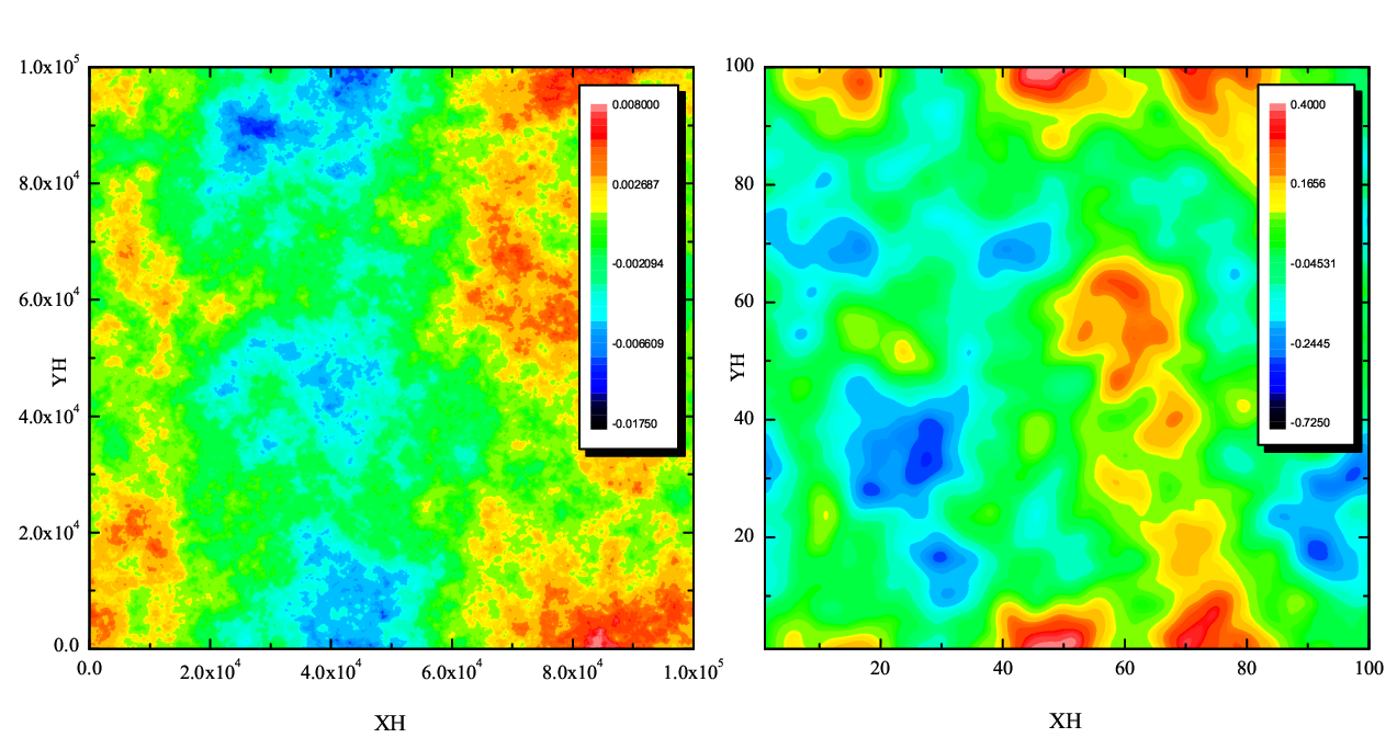
Therefore, for the amplitude of perturbation on large scale will inevitably arrive at at certain time of cycles. We only show it in Fig.3, since the linear perturbation approximation is not reliable when , and in this case, the nonlinear effect will become important and the coupling between modes has to be considered. However, it can be expected that the enhancement of nonlinear effect will bring to 1 faster. This means that on the corresponding scale the perturbation will be large enough so that will destroy the homogeneity of background. We illustrate this effect of the perturbation on background by transforming in Fig.3 into in position space plotted in Fig.4.
We can see that when the universe is fragmentized into large number of small regions. In this case, the initially global homogeneous universe will become highly inhomogeneous. Thus it can be hardly imagined that the different regions of global universe will evolve synchronously, even if it is homogenous in the previous cycle. Thus the cycle of global universe will ultimately end. The similar phenomenon was also discussed in [41], however, in which since the bounce is singular the special mode mixing has to be applied for the amplification of , e.g.[38],[39],[40]. Here, the bounce builded is nonsingular, thus the evolution of perturbations through cycles can be exactly studied by numerical method.
In general, as long as the curvature perturbation on large scale is amplified cycle by cycle actually occurs, it is hardly possible that the global universe is eternal cyclic. We only consider the evolution of curvature perturbation, the effect of the increasing of other perturbations on cyclic universe has been also studied, e.g.[42]. These results mean that the reliability of some models of cyclic universe might need to be reevaluated.
However, it can be noticed that for the universe with increasing cycle, the regions split can be larger. When the length of local regions split is larger than the Hubble scale at the corresponding time, these regions will possibly evolve independently, as long as inside the corresponding regions the background is homogeneous. In principle, such different local regions correspond to different universes [43],[44], each of which is controlled by local physical equations and might be fragmentized again after itself cycles. In this case, the number of local universes will increase cycle by cycle. Thus we can have a cyclic multiverse scenario, as argued in [15],[16]. This argument in some sense indicates that in cyclic cosmology a gradually increasing cycle is significant for the continuance of cycle, however, in this case, the cycle will continue only at local regions, which is homogeneous. This scenario can be distinguished from that in chaotic eternal inflation [45, 46], in which the inflationary multiverse is induced by the large quantum fluctuation of inflaton field, which occurs efold by efold. However, the cyclic multiverse is induced by the cyclic amplification of perturbation on large scale, which is in classical sense, and occurs cycle by cycle.
In conclusion, we have analytically and numerically showed that through the cycles with nonsingular bounce the amplitude of curvature perturbations on large scale will be amplified and the power spectrum will be redden. In some sense, this amplification will eventually destroy the homogeneity of background, which might lead to the ultimate end of cycles of global universe. However, it can be argued that for the model with increasing cycle, the global universe will possibly evolve into a fissiparous multiverses after one or several cycles, in which the cycles will continue only at corresponding local regions, inside which the background is homogeneous.
Acknowledgments We thank for Y.F. Cai and A. Mazumdar helpful discussions and comments. This work is supported in part by NSFC under Grant No:10775180, 11075205, in part by the Scientific Research Fund of GUCAS(NO:055101BM03), in part by National Basic Research Program of China, No:2010CB832804
References
- [1] R.C. Tolman, Relativity, Thermodynamics and Cosmology, (Oxford U. Press, Clarendon Press, 1934).
- [2] P.J. Steinhardt, N. Turok, Science 296, (2002) 1436; Phys. Rev. D65 126003 (2002).
- [3] J. Barrow, M. P. Dabrowski, Mon. Not. R. Astr. Soc. 275, 850 (1995).
- [4] N. Kanekar, V. Sahni, Y. Shtanov, Phys. Rev. D63, 083520 (2001).
- [5] Y.S. Piao, Phys. Rev. D70, 101302 (2004); Y.S. Piao, Y.Z. Zhang, Nucl. Phys. B725, 265 (2005).
- [6] J.E. Lidsey, D.J. Mulryne, N.J. Nunes, R. Tavakol, Phys. Rev. D70, 063521 (2004).
- [7] T. Clifton, J.D. Barrow, Phys. Rev. D75, 043515 (2007).
- [8] H.H. Xiong, Y.F. Cai, T. Qiu, Y.S. Piao, X.M. Zhang, Phys. Lett. B666, 212 (2008).
- [9] X. Zhang, Eur. Phys. J. C60, 661 (2009).
- [10] J.L. Lehners, P.J. Steinhardt, Phys. Rev. D79, 063503 (2009).
- [11] T. Biswas, S. Alexander, Phys. Rev. D80, 043511 (2009).
- [12] T. Biswas, A. Mazumdar, Phys. Rev. D80, 023519 (2009).
- [13] Y.F. Cai, E.N. Saridakis JCAP 0910, 020 (2009).
- [14] M. Novello, S.E.P. Bergliaffa, Phys. Rept. 463, 127 (2008).
- [15] Y.S. Piao, Phys. Lett. B677, 1 (2009).
- [16] Y.S. Piao, arXiv:1001.0631.
- [17] M.S. Turner, Phys. Rev. D28, 1243 (1983).
- [18] J.M. Cline, S. Jeon, G. D. Moore Phys. Rev. D70, 043543 (2004).
- [19] T. Biswas, A. Mazumdar, W. Siegel, JCAP 0603, 009 (2006).
- [20] T. Biswas, T. Koivisto, A. Mazumdar, arXiv:1005.0590.
- [21] D. Wands, Phys. Rev. D60, 023507 (1999).
- [22] F. Finelli, R. Brandenberger, Phys. Rev. D65, 103522 (2002).
- [23] A.A. Starobinsky, JETP Lett. 30, 682 (1979).
- [24] L.E. Allen, D. Wands, Phys. Rev. D70, 063515 (2004).
- [25] V. Bozza, G. Veneziano, Phys. Lett. B625, 177 (2005).
- [26] F. Finelli, P. Peter, N. Pinto-Neto, Phys. Rev. D77, 103508 (2008).
- [27] Y.F.Cai, T. Qiu, R. Brandenberger, X.M. Zhang, Phys. Rev. D80, 023511 (2009).
- [28] Y.S. Piao, B. Feng, X.M. Zhang, Phys. Rev. D69, 103520 (2004).
- [29] Y.S. Piao, S. Tsujikawa, X.M. Zhang, Class. Quant. Grav. 21, 4455 (2004).
- [30] Y.S. Piao, Phys. Rev. D71, 087301 (2005).
- [31] V.F. Mukhanov, JETP lett. 41, 493 (1985); Sov. Phys. JETP. 68, 1297 (1988).
- [32] H. Kodama, M. Sasaki, Prog. Theor. Phys. Suppl. 78 1 (1984).
- [33] V. Mukhanov, “Physical Foundations of Cosmology”, (Cambridge University Press, 2005).
- [34] Y.S. Piao, Phys. Lett. B606, 245 (2005); Y.S. Piao, Y.Z. Zhang, Phys. Rev. D70, 043516 (2004).
- [35] J. Khoury, P.J. Steinhardt, Phys. Rev. Lett. 104, 091301 (2010).
- [36] T. Biswas, A. Mazumdar, A. Shafieloo, arXiv:1003.3206.
- [37] R. Brandenberger, Phys. Rev. D80, 023535 (2009).
- [38] D.H. Lyth, Phys. Lett. B524, 1 (2002); Phys. Lett. B 526, 173 (2002).
- [39] R. Durrer and F. Vernizzi, Phys. Rev. D66, 083503 (2002).
- [40] S. Tsujikawa, R. Brandenberger, F. Finelli, Phys. Rev. D66, 083513 (2002).
- [41] J.K. Erickson, S. Gratton, P.J. Steinhardt, N. Turok, Phys. Rev. D75, 123507 (2007).
- [42] J.D. Barrow, K. Yamamoto, arXiv:1004.4767.
- [43] B. Carr, S.W. Hawking, Mon. Not. R. Astro. Soc. 168, 399 (1974).
- [44] D. Wands, K.A. Malik, D.H. Lyth, A.R. Liddle, Phys. Rev. D62, 043527 (2000).
- [45] A. Vilenkin, Phys. Rev. D27, 2848 (1983).
- [46] A. Linde, Phys. Lett. B175, 395 (1986).