Topological Black Holes in Gauss-Bonnet Gravity with conformally invariant Maxwell source
Abstract
In this paper, we present a class of rotating solutions in Gauss–Bonnet gravity in the presence of cosmological constant and conformally invariant Maxwell field and study the effects of the nonlinearity of the Maxwell source on the properties of the spacetimes. These solutions may be interpret as black brane solutions with inner and outer event horizons provide that the mass parameter is greater than an extremal value , an extreme black brane if and a naked singularity otherwise. We investigate the conserved and thermodynamics quantities for asymptotically flat and asymptotically with flat horizon. We also show that the conserved and thermodynamic quantities of these solutions satisfy the first law of thermodynamics.
pacs
04.40.Nr, 04.20.Jb, 04.70.Bw, 04.70.DyI Introduction
The presence of higher curvature terms can be seen in many theories such as renormalization of quantum field theory in curved spacetime [1], or in construction of low energy effective action of string theory [2] and so on. These examples motivate one to consider the more general class of gravitational action
where , and are Ricci scalar, Ricci and Riemann tensor respectively. Among the higher curvature gravity theories, the so called Lovelock gravity is quite special, whose Lagrangian consist of the dimensionally extended Euler densities. This Lagrangian is obtained by Lovelock as he tried to calculate the most general tensor that satisfies properties of Einstein’s tensor in higher dimensions [3]. Since the Lovelock tensor does not contain derivatives of metrics of order higher than second, the quantization of linearized Lovelock theory is free of ghosts [4]. The gravitational action of Lovelock theory can be written as [3]
| (1) |
where denotes integer part of , is an arbitrary constant and is the Euler density of a -dimensional manifold,
| (2) |
In Eq. (2) is the generalized totally anti-symmetric Kronecker delta. It is worthwhile to mention that in dimensions, all terms for which are identically equal to zero, and the term is a topological term. So, only terms for which are contributing to the field equations. In this paper we want to restrict ourself to the first three terms of Lovelock gravity. The first term is the cosmological term and the second and third terms are the Einstein and second order Lovelock (Gauss-Bonnet) terms respectively.
In the last decades a renewed interest appears in Lovelock gravity. In particular, exact static spherically symmetric black hole solutions of the Gauss-Bonnet gravity have been found in Ref. [4, 5]. Exact solutions of static and rotating of the Maxwell-Gauss-Bonnet and Born-Infeld-Gauss-Bonnet models have been investigated in Ref. [6, 7, 8, 9, 10, 11]. The thermodynamics of the uncharged static spherically black hole solutions has been considered in [12]. Properties of solutions with nontrivial topology have been studied in [13, 14] and charged black hole solutions have been found in [6, 15].
In the conventional, straightforward generalization of the Maxwell field to higher dimensions one essential property of the electromagnetic field is lost, namely, conformal invariance. The first black hole solution derived for which the matter source is conformally invariant is the Reissner-Nordström solution in four dimensions. Indeed, in this case the source is given by the Maxwell action which enjoys the conformal invariance in four dimensions. Massless spin- fields have vanishing classical stress tensor trace in any dimension, while scalars can be “improved” to achieve , thereby guaranteeing invariance under the special conformal (or full Weyl) group, in accord with their scale-independence [16, 17, 18]. Maxwell theory can be studied in a gauge which is invariant under conformal rescalings of the metric, and firstly, has been proposed by Eastwood and Singer [19]. Also, Poplawski [20] have been showed the equivalence between the Ferraris–Kijowski and Maxwell Lagrangian results from the invariance of the latter under conformal transformations of the metric tensor. Quantized Maxwell theory in a conformally invariant gauge have been investigated by Esposito [21]. Also, there exists a conformally invariant extension of the Maxwell action in higher dimensions (Generalized Maxwell Field, GMF), if one uses the lagrangian of the gauge field in the form [22]
| (3) |
where is the Maxwell tensor and is an arbitrary constant. It is straightforward to show that the action (3) is invariant under conformal transformation ( and ) and for , the action (3) reduces to the Maxwell action as it should be. The energy-momentum tensor associated to is given by
| (4) |
where and it is easy to show that . In what follows, we consider the action (3) as the matter source coupled to the Gauss-Bonnet gravity. The idea is to take advantage of the conformal symmetry to construct the analogues of the four-dimensional Reissner-Nordström black hole solutions in higher dimensions. The form of the energy-momentum tensor (4), automatically restricts the dimensions to be only multiples of four.
The main aim of this work is to present analytical solutions for typical class of rotating spacetime in Gauss-Bonnet theory coupled to conformally invariant Maxwell source with negative cosmological constant. As we show later, these solutions have some interesting properties, specially in the electromagnetic fields, which do not occur in Gauss-Bonnet gravity in the present of ordinary Maxwell field. In this paper we discuss black hole solutions of Gauss-Bonnet-conformally invariant Maxwell source and investigate their properties and calculate the conserved and thermodynamics quantities.
The outline of our paper is as follows. In next Section, we present the basic field equations and general formalism of calculating the conserved quantities. In section III, we present the topological black hole of Gauss-Bonnet gravity in the presence of conformally invariant Maxwell source. Then, we calculate the thermodynamic quantities of asymptotically flat solutions and investigate the first law of thermodynamics. In next subsection III.3 we introduce the rotating solutions with flat horizon and compute the thermodynamic and conserved quantities of them. We also perform a stability analysis of this solutions both in canonical and grand canonical ensemble. Finally, we finish our paper with some concluding remarks.
II Field Equations in Gauss-Bonnet Gravity with Conformally Invariant Maxwell Source
The action of Gauss-Bonnet gravity in the presence of conformally invariant electromagnetic field is
| (5) | |||||
where is the negative cosmological constant for asymptotically AdS solutions and is the Gauss-Bonnet coefficient with dimension . The second integral in Eq. (5) is the Gobbons-Hawking surface term and its counterpart for the Gauss-Bonnet gravity which is chosen such that the variational principle is well defined [23]. In this term, is induced metric on the boundary , is trace of extrinsic curvature of the boundary, is Einstein tensor of the metric , and is trace of the tensor
| (6) |
Varying the action with respect to the metric tensor and electromagnetic field the equations of gravitation and electromagnetic fields are obtained as
| (7) |
| (8) |
where is the Einstein tensor and is the divergence-free symmetric tensor
| (9) |
Hereafter we set without loss of generality and consequently the energy density (the component of the energy-momentum tensor in the orthonormal frame) is positive.
Equation (7) does not contain the derivative of the curvatures, and therefore the derivatives of the metric higher than two do not appear. In general the action is diverged when evaluated on solutions, as is the Hamiltonian and other associated conserved charges. For asymptotically solutions, one can instead deal with these divergences via the counterterm method inspired by correspondence [24]. In the present context this correspondence furnishes a means for calculating the action and conserved quantities intrinsically by adding additional terms on the boundary that are curvature invariants of the induced metric. Although there may exist a very large number of possible invariants one could add in a given dimension, only a finite number of them are non vanishing as the boundary is taken to infinity. Its many applications include computations of conserved quantities for black holes with rotation, various topologies, rotating black strings with zero curvature horizons and rotating higher genus black branes [25]. Usually, the counterterm method applies for the case of a specially infinite boundary, but it was also employed for the computation of the conserved and thermodynamic quantities in the case of a finite boundary [26]. Thus, in order to extract the physically relevant information, the on-shell action has to be renormalized by adding counterterms, which cancel the infinities of in the absence of matter. This counterterms is [27]
| (10) | |||||
where is the step function which is equal to one for and zero otherwise. Thus, the total finite action can be written as a linear combination of the gravity term and the counterterm . Having the total finite action, one can use the Brown and York definition of energy-momentum tensor [28] to construct a divergence free stress-energy tensor. This tensor is
| (11) | |||||
When there is a Killing vector field on the boundary, the quasilocal conserved quantities associated with the stress tensors of Eq. (11) can be written as
| (12) |
where is the determinant of the metric , and is the timelike unit normal vector to the boundary . In the context of counterterm method, the limit in which the boundary becomes infinite () is taken, and the counterterm prescription ensures that the action and conserved charges are finite.
III Black Hole Solutions:
III.1 Topological Black Holes
Here we want to obtain the -dimensional static solutions of Eqs. (7) and (8). We assume that the metric has the following form:
| (13) |
where
| (14) |
which represents the line element of an -dimensional hypersurface with constant curvature and volume .
Using Eq. (8), one can show that the vector potential, in -dimensions, can be written as
| (15) |
where is an integration constant which is related to the charge parameter. The conformally invariant Maxwell equation implies that the electric field in -dimensions is proportional to and given by
| (16) |
One may show that the metric function
| (17) |
where
satisfies the field equations (7), where is the mass parameter. The metric function is real in the whole range for uncharged solution (), provided that . For charged real solution one needs a transformation to make them real [7, 29]. In the other word, is real only in the range , where is the largest real root of the following equation
| (18) |
In order to restrict spacetime to the region , we introduce a new radial coordinate such as [7]
| (19) |
With this new coordinate, the above metric becomes
| (20) |
where is the same as Eq. (14) and the functions and change to
| (21) |
| (22) |
| (23) |
In order to consider the asymptotic behavior of the solution, we put where the metric function reduces to
| (24) |
Equation (24) shows that the asymptotic behavior of the solution is AdS or dS provided or . The case of asymptotic flat solutions () is permitted only for . It easy to show that in the vicinity of
and thus, the metric given by Eqs. (20), (22) and (23) has an essential timelike singularity at . Seeking possible black hole solutions, we turn to looking for the existence of horizons. The event horizon(s), if there exists any, is (are) located at the root(s) of . Denoting the largest real root of by , we consider first the case that has only one real root (see Fig. 1, continuous line). In this case is minimum at and therefore . That is,
| (25) |

One can find the extremal value of mass, , in terms of parameters of metric function by finding from Eq. (25) and inserting it into equation . Then, the metric of Eqs. (20), (22) and (23) presents a black hole solution with inner and outer event horizons provided , an extreme black hole for [temperature is zero since it is proportional to ] and a naked singularity otherwise. It is a matter of calculation to show that for becomes
| (26) |
The Hawking temperature of the black holes can be easily obtained by requiring the absence of conical singularity at the horizon in the Euclidean sector of the black hole solutions. One obtains
| (27) | |||||
It is worth to note that is zero for .
III.2 Thermodynamics of Asymptotically Flat Black Holes for
In this section, we consider the thermodynamics of spherically symmetric black holes which are asymptotically flat. First of all we focus on entropy. Usually entropy of black holes satisfies the so-called area law of entropy which states that the black hole entropy equals to one-quarter of horizon area. It applies to all kind of black holes and black strings of Einstein gravity [30]. However, in higher derivative gravity the area law of entropy is not satisfied in general [31]. It is known that the entropy in of asymptotically flat solutions of Lovelock gravity is [32]
| (28) |
where the integration is done on the -dimensional spacelike hypersurface of Killing horizon, is the induced metric on it, is the determinant of and is the th order Lovelock Lagrangian of . Denoting the volume of the boundary at constant and by , the entropy in Gauss-Bonnet gravity per unit volume is
| (29) |
where is the Ricci scalar for the induced metric on the -dimensional horizon. It is a matter of calculation to show that the entropy of black holes is
| (30) |
The charge per unit volume of the black hole can be found by calculating the flux of the electric field at infinity, yielding
| (31) |
The electric potential , measured at infinity with respect to the horizon, is defined by
| (32) |
where is the null generator of the horizon. One finds
| (33) |
The ADM (Arnowitt–Deser–Misner) mass of black hole can be obtained by using the behavior of the metric at large . According to the definition of mass due to Abbott and Deser [33], the mass per unit volume of the solutions () is
| (34) |
We now investigate the first law of thermodynamics. Using the expression for the entropy, the charge, and the mass given in Eqs. (30), (31) and (34), and the fact that , one obtains
| (35) | |||||
where is the real root of Eq. (30) which is a function of . One may then regard the parameters and as a complete set of extensive parameters for the mass and define the intensive parameters conjugate to them. These quantities are the temperature and the electric potential
| (36) |
Computing and and using chain rule, it is easy to show that the intensive quantities calculated by Eq. (36) coincide with Eqs. (27) and (33) respectively. Thus, the thermodynamic quantities calculated in Eqs. (27) and (33) satisfy the first law of thermodynamics,
| (37) |
III.3 Thermodynamics of Asymptotically AdS Rotating Black Branes with Flat Horizon
Now, we want to endow our spacetime solution (13) for with a global rotation. In order to add angular momentum to the spacetime, we perform the following rotation boost in the planes
| (38) |
for , where is the integer part of . The maximum number of rotation parameters is due to the fact that the rotation group in dimensions is and therefore the number of independent rotation parameters is . Thus the metric of asymptotically AdS rotating solution with rotation parameters for flat horizon can be written as
| (39) | |||||
where . Because of the periodic nature of , the transformation 38 is not a proper coordinate transformation on the entire manifold. Therefore, the static and rotating metrics can be locally mapped into each other but not globally, and so they are distinct [34]. We show that the intensive and extensive quantities depend on the rotation parameters. Using Eq. (8), one can show that the vector potential can be written as
| (40) |
One can obtain the temperature and angular momentum of the event horizon by analytic continuation of the metric. One obtains
| (41) |
| (42) |
Next, we calculate the electric charge and potential of the solutions. The electric charge per unit volume can be found by calculating the flux of the electric field at infinity, yielding
| (43) |
Using Eq. (32) and the fact that is the null generator of the horizon, the electric potential is obtained as
| (44) |
III.3.1 Finite Action and Conserved quantities of the solutions
Here, we calculate the action and conserved quantities of the black brane solutions. For asymptotically AdS of our solutions with flat boundary, , the finite action, , reduce to [29, 26]
| (45) |
where is
| (46) |
One may note that reduces to as goes to zero. Using Eqs. (5) and (45), the finite action per unit volume can be calculated as
| (47) |
Using the Brown-York method [28], the finite energy-momentum tensor is
| (48) |
and by using Eq. (12), the conserved quantities associated with the Killing vectors and are
| (49) | |||||
| (50) |
which are the mass and angular momentum per unit volume of the solutions.
III.3.2 First law of thermodynamics and Stability of the solutions
Calculating all the thermodynamic and conserved quantities of the black brane solutions, we now check the first law of thermodynamics for our solutions with flat horizon. We obtain the mass as a function of the extensive quantities , , and . Using the expression for charge mass, angular momenta and entropy given in Eqs. (43), (49), (50), (52) and the fact that , one can obtain a Smarr-type formula as
| (53) |
where and is the positive real root of the following equation
| (54) |
One may then regard the parameters , ’s, and as a complete set of extensive parameters for the mass and define the intensive parameters conjugate to them. These quantities are the temperature, the angular velocities, and the electric potential
| (55) |
Straightforward calculations show that the intensive quantities calculated by Eq. (55) coincide with Eqs. (41), (42) and (44). Thus, these quantities satisfy the first law of thermodynamics

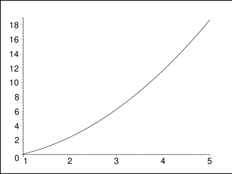
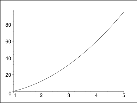
Finally, we investigate the local stability of charged rotating black brane solutions of Gauss-Bonnet gravity in the presence of conformally invariant Maxwell source in the canonical and grand canonical ensembles. In the canonical ensemble, the positivity of the heat capacity and therefore the positivity of is sufficient to ensure the local stability. It is easy show that
| (56) |
where
| (57) | |||||
The heat capacity is positive for , where the temperature is positive. This fact can be seen easily for , where the is positive and then is positive too. Also, one may see from Figs. (2, 3 and 4) that the increases as increases, and therefore it is always positive. Thus the condition for thermal equilibrium in the canonical ensemble is satisfied.
In grand canonical ensemble, the positivity of the determinant of Hessian matrix of with respect to its extensive variables , , is sufficient to ensure the local stability. It is a matter of calculation to show that the determinant of is
| (58) |
Equation (58) shows that the determinant of Hessian matrix is positive, and therefore the solutions are stable in grand canonical ensemble too. This phase behavior is commensurate with the fact that there is no Hawking-Page transition for a black object whose horizon is diffeomorphic to and therefore the system is always in the high temperature phase [35].
IV Closing Remarks
In this paper, we presented a class of rotating solutions in Gauss–Bonnet gravity in the presence of conformally invariant Maxwell field and investigated the effects of the nonlinearity of the electromagnetic fields on the properties of the solutions. These solutions may be interpreted as black brane solutions with inner and outer event horizons provided that the mass parameter is greater than an extremal value , an extreme black brane if and a naked singularity otherwise. We considered thermodynamics of asymptotically flat solutions and found that the first law of thermodynamics is satisfied by the conserved and thermodynamic quantities of the black hole. We also considered the rotating solution with flat horizon and computed the action and conserved quantities of it through the use of counterterm method. We found that the entropy obeys the area law for black branes with flat horizon. We obtained a Smarr-type formula for the mass of the black brane as a function of the entropy, the charge, and the angular momenta, and found that the conserved and thermodynamics quantities satisfy the first law of thermodynamics. We also studied the phase behavior of the ()-dimensional rotating black branes and showed that there is no Hawking-Page phase transition in spite of the angular momenta of the branes and the presence of the conformally invariant Maxwell field. Indeed, we calculated the heat capacity and the determinant of the Hessian matrix of the mass with respect to , J, and of the black branes and found that they are positive for all the phase space, which means that the brane is locally stable for all the allowed values of the metric parameters.
Acknowledgements.
This work has been supported financially by Research Institute for Astronomy and Astrophysics of Maragha.References
- [1] N. D. Birrell and P. C. W. Davies, Quantum Fields in Curved Space, (Cambridge University Press, Cambridge, England, 1982).
- [2] M. B. Greens, J. H. Schwarz and E. Witten, Superstring Theory, (Cambridge University Press, Cambridge, England, 1987); D. Lust and S. Theusen, Lectures on String Theory, (Springer, Berlin, 1989); J. Polchinski, String Theory, (Cambridge University Press, Cambridge, England, (1998).
- [3] D. Lovelock, J. Math. Phys. 12, 498 (1971); N. Deruelle and L. Farina-Busto, Phys. Rev. D 41, 3696 (1990); G. A. MenaMarugan, Phys. Rev. D 46, 4320 (1992); 4340 (1992).
- [4] D. G. Boulware and S. Deser, Phys. Rev. Lett. 55, 2656 (1985); J. T. Wheeler, Nucl. Phys. B 268, 737 (1986).
- [5] D. Astefanesei, N. Banerjee and S. Dutta JHEP 0811, 070 (2008).
- [6] D. L. Wiltshire, Phys. Lett. B 169, 36 (1986); D. L. Wiltshire, Phys. Rev. D 38, 2445 (1988).
- [7] M. H. Dehghani and S. H. Hendi, Int. J. Mod. Phys. D 16, 1829 (2007).
- [8] M. H. Dehghani, Phys. Rev. D 67, 064017 (2003).
- [9] M. H. Dehghani, Phys. Rev. D 70, 064019 (2004).
- [10] M. H. Dehghani, Phys. Rev. D 69 064024 (2004).
- [11] M. H. Dehghani and M. Shamirzaie, Phys. Rev. D 72, 124015 (2005).
- [12] R. C. Myers and J. Z. Simon, Phys. Rev. D 38, 2434 (1988); R. C. Myers, Nucl. Phys. B 289, 701 (1987).
- [13] R. G. Cai, Phys. Rev. D 65, 084014 (2002).
- [14] M. H. Dehghani and R. B. Mann, Phys. Rev. D 72, 124006 (2005); M. H. Dehghani and S. H. Hendi, Phys. Rev. D 73, 084021 (2006).
- [15] M. Cvetic, S. Nojiri and S. D. Odintsov, Nucl. Phys. B 628, 295 (2002); S. Nojiri and S. D. Odintsov, Phys. Lett. 521B, 87 (2001).
- [16] S. Deser and A. Schwimmer, Int. J. Mod. Phys. B 8, 3741 (1994).
- [17] G. Esposito and C. Stornaiolo, Class. Quant. Grav. 17, 1989 (2000); G. Esposito and C. Stornaiolo, Nucl. Phys. Proc. Suppl. 88, 365 (2000)
- [18] C. Codirla and H. Osborn, Annals Phys. 260, 91 (1997).
- [19] M. Eastwood and M. Singer, Phys. Lett. A 107, 73 (1985).
- [20] N. J. Poplawski, Int. J. Mod. Phys. A 23, 567 (2008).
- [21] G. Esposito, Phys. Rev. D56, 2442 (1997).
- [22] M. Hassaine and C. Martinez, Phys. Rev. D. 75, 027502 (2007); M. Hassaine and C. Martinez, Class. Quant. Grav. 25, 195023 (2008); H. Maeda, M. Hassaine and C. Martinez, Phys. Rev. D 79, 044012 (2009).
- [23] R. C. Myers, Phys. Rev. D 36, 392 (1987); S. C. Davis, Phys. Rev. D 67, 024030 (2003).
- [24] J. Maldacena, Adv. Theor. Math. Phys., 2, 231 (1998); E. Witten, Adv. Theor. Math. Phys., 2, 253 (1998); O. Aharony, S. S. Gubser, J. Maldacena, H. Ooguri and Y. Oz, Phys. Rept., 323, 183 (2000).
- [25] M. H. Dehghani, Phys. Rev. D 66, 044006 (2002); Phys. Rev. D 65, 124002 (2002); M. H. Dehghani and A. Khodam-Mohammadi, Phys. Rev. D 67, 084006 (2003).
- [26] M. H. Dehghani and R. B. Mann, Phys. Rev. D 64, 044003 (2001); M. H. Dehghani, Phys. Rev. D 65, 104030 (2002); M. H. Dehghani and H. KhajehAzad, Can. J. Phys. 81, 1363 (2003).
- [27] P. Kraus, F. Larsen and R. Siebelink, Nucl. Phys. B 563, 259 (1999).
- [28] J. D. Brown and J. W. York, Phys. Rev. D 47, 1407 (1993).
- [29] M. H. Dehghani, G. H. Bordbar and M. Shamirzaie, Phys. Rev. D 74, 064023 (2006).
- [30] J. D. Bekenstein, Phys. Rev. D 7, 2333 (1973); S. W. Hawking and C. J. Hunter, Phys. Rev. D 59 044025 (1999); S. W. Hawking, C. J. Hunter and D. N. Page, Phys. Rev. D 59, 044033 (1999); R. B. Mann, Phys. Rev. D 60, 104047 (1999); Phys. Rev. D 61, 084013 (2000); C. J. Hunter, Phys. Rev. D 59, 024009 (1999).
- [31] M. Lu and M. B. Wise, Phys. Rev. D 47, 3095 (1993); M. Visser, Phys. Rev. D 48, 583 (1993).
- [32] T. Jacobson and R. C. Myers, Phys. Rev. Lett. 70, 3684 (1993); R. M. Wald, Phys. Rev. D 48, R3427, (1993); M. Visser, Phys. Rev. D 48, 5697 (1993); T. Jacobson, G. Kang and R. C. Myers, Phys. Rev. D 49, 6587,(1994); V. Iyer and R. M. Wald, Phys. Rev. D 50, 846 (1994).
- [33] L. F. Abbott and S. Deser, Nucl. Phys. B 195, 76 (1982).
- [34] J. Stachel, Phys. Rev. D 26, 1281 (1982).
- [35] E. Witten, Adv. Theor. Math. Phys. 2, 505 (1998).