Di-neutron clustering and deuteron-like tensor correlation in nuclear structure focusing on ¹¹Li

There are many experimental data indicating that the ¹¹Li nucleus has a halo structure. A schematic picture of the halo structure is shown in Fig.1. The halo structure of ¹¹Li was discovered as an anomalously large reaction cross section of this nucleus with target nuclei. The matter radii extracted from the reaction cross sections and other standard methods are shown in Fig.2. We can see from this figure that the matter radius of ¹¹Li is much larger than that of the neighboring nucleus ⁹Li. The matter radius of ¹¹Li corresponds to those of medium mass nuclei. If we were to pick up nuclei, whose radii are suddenly increased from the neighboring nuclei, they are ⁶He, ¹¹Be and ¹⁴Be in addition to ¹¹Li. Detailed studies on these sudden jumps of the matter radii made these phenomena as caused by the halo formation.

There are many experiments performed on the halo structure of unstable nuclei. Out of all these experiments, those of ¹¹Li are very interesting due to important nuclear many body physics behind the experimental data. In order to find the reason of the sudden increase, experiments were performed for the neutron separation momentum distributions. The momentum distributions of neutron separation were measured experimentally by Kobayashi et al. [2] by bombarding unstable nuclei on some stable target nuclei. The momentum distribution for the case of ¹¹Li is much narrower than other cases. The narrowness of the momentum distribution is related with large extension of the neutron distributions due to the uncertainty principle. Hence, this is a data showing directly the halo structure or at least a large spatial extension of the neutron distribution in ¹¹Li. As for the structure of ¹¹Li, there was an experiment performed by Simon et al. [3], who bombarded ¹¹Li on a carbon target and measure the momentum distribution of the ¹⁰Li fragments. From the shape of the distribution, the $(1s_{1/2})^{2}$ contribution to the mixture of $(1s_{1/2})^{2}$ and $(0p_{1/2})^{2}$ components was determined to be $(45\pm 10)\%$.

If there is a halo structure, we may expect an interesting excitation mode of ¹¹Li. If the core nucleus ⁹Li is surrounded by neutrons in the nuclear halo region, there is a possibility of making oscillation of the core nucleus in the neutron sea. This is called a soft dipole resonance to be excited by photo-disintegration as shown in Fig. 3 [4, 5]. The excitation energy is expected around a few MeV as compared to the standard giant $E1$ resonance of a few tens MeV. There are several experiments of Coulomb excitation of ¹¹Li. We show the most recent experimental data on Coulomb excitation taken by Nakamura et al. in Fig.4 [6]. There is a bump structure just above the threshold energy. However, it is still debated if the bump structure is caused by the soft dipole resonance or not due to the complicated nuclear structure of ¹¹Li. There are many other experimental data on ¹¹Li as the magnetic moment and quadrupole moment. These experimental data will be presented together with theoretical results later.

We should also see experimental data for ¹⁰Li, which is the neighboring nucleus, although this nucleus is unbound. We list the neutron single and double separation energies in ^9,10,11Li in Table 1. The two neutron separation energy in ¹¹Li is very small as 0.32MeV. The separation energies in ⁹Li are large and this nucleus should be considered as a standard shell model type nucleus. In ¹⁰Li, the single neutron separation energy is $-0.3$ MeV, indicating this nucleus is not stable. This resonance structure seems to have positive parity and is assigned to have the $(p_{3/2})_{\pi}(p_{1/2})_{\nu}$ structure. At the same time, there are few informations on virtual states. There is an experimental data on neutron scattering with ⁹Li at the threshold energy [7]. The scattering length comes out to be $a\sim-20$ fm, which is comparable with the one of neutron-neutron scattering $a=-18.5\pm 0.4$ fm [8]. Hence, the large scattering length indicates the existence of strong attraction in the s-wave channel, which is closed to the condition of forming a bound state in the free space. This means that the s-state structure appears close to the threshold energy of ⁹Li + $n$.

The halo structure was completely new in nuclear physics community. Hence, there were many theoretical studies to describe this interesting phenomenon. We have recognized immediately that the standard shell model approach badly fails due to the fact that the two additional neutrons in ¹¹Li ought to enter in the $p_{1/2}$ neutron orbit but not in the $s_{1/2}$ orbit due to the N=8 magic structure. Hence, most of theoretical studies introduce some phenomenology to bring down the $s_{1/2}$ orbit. For example, in the work of Thompson and Zhukov [9], they treat ⁹Li as a core and add two neutrons by taking state dependent neutron-core interactions. The additional attraction for s-wave component makes the $(s_{1/2})^{2}$ state energetically close to the $(p_{1/2})^{2}$ state. In this case, the $(s_{1/2})^{2}$ state has a large component in the ground state, which provides the halo structure for ¹¹Li.

There is a theoretical study on the pairing property and the E1 excitation in ¹¹Li by Esbensen and Bertsch [10]. In their study, it is essential to bring down the $s_{1/2}$ orbit to reproduce the experimental E1 excitation spectrum. As for the pairing correlation, there are many studies to describe ¹¹Li as the BCS state. In the study of Meng and Ring [11], they describe ¹¹Li in terms of a relativistic Hartree-Bogoliubov model. In this study, they can include the continuum effect in their pairing correlations. In the relativistic Hartree-Bogoliubov model, the s-wave contribution comes out to be about a quarter of the p-wave contribution for the paired two neutrons. We need more participation of the s-wave component as compared to the finding of the experimental data of Simon et al. [3].

There is another interpretation on the halo structure as due to deformation. In the work of Varga, Suzuki and Lovas [12], they try to break the ⁹Li core and introduce the cluster structure. The wave function of ¹¹Li is written as ⁴He$+t+4n$ and take the interaction among them by a phenomenological central interaction. In this way, they can introduce the effect of the deformation and pairing correlations among the nucleons. The deformation effect provides a large matter radius and some s-wave component in the wave function.

The theoretical challenge on the halo structure is therefore summarized as follows. There are many indications that the s-wave component is very large in the ground state wave function. Hence, we have to find a mechanism to bring down the $s_{1/2}$ orbit with the amount to wash out the N=8 magic structure. The pairing properties are also very important to cause admixture of $(p_{1/2})^{2}$ and $(s_{1/2})^{2}$ states. In the halo nucleus, we ought to consider the di-neutron pairing correlation in a small nuclear matter density. All these new phenomena should be understood in terms of the many body framework with the nucleon-nucleon interaction.

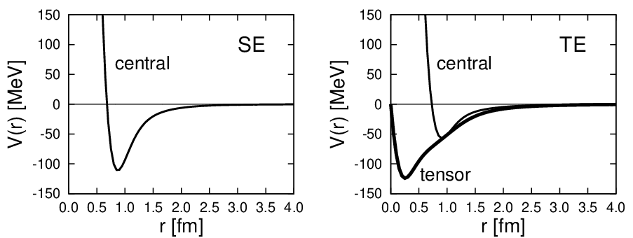
We should learn the properties of the nucleon-nucleon interaction in order to understand the halo structure in ¹¹Li. To this end, we would like to show the central and the tensor interactions in the ${}^{3}S_{1}$ channel of the AV8’ potential [13], which are shown in Fig. 5. In the central interaction, there are strong hard core (short range repulsive interaction) and intermediate range attraction of moderate strength. As for the tensor interaction, the long range part drops with the pion range, while the short range part increases until $0.2$ fm and goes to zero at the origin due to the form-factor coming from the nucleon finite size. On the other hand, we have the similar structure for the central interaction in the ${}^{1}S_{0}$ channel, where there is a strong hard core due to the short range quark dynamics. In this channel, there is no tensor contribution due to zero total spin. The deuteron-like tensor correlation is produced by the $NN$ interaction in the ${}^{3}S_{1}$ channel, while the di-neutron clustering is produced by the $NN$ interaction in the ${}^{1}S_{0}$ channel.

In order to understand the role of the hard core and the tensor interaction, let us solve the Schrödinger equation for the deuteron by using the AV8’ nucleon-nucleon interaction. The wave function of the deuteron is written as

$\displaystyle\Psi_{d}$

$\displaystyle=$

$\displaystyle u(r)[Y_{0}(\hat{r})\otimes\chi_{1}(\sigma_{1}\sigma_{2})]_{1M}+w(r)[Y_{2}(\hat{r})\otimes\chi_{1}(\sigma_{1}\sigma_{2})]_{1M}~.$

(1)

The deuteron wave function is written by the $s$-wave and $d$-wave components. The tensor interaction mixes these two components. In Fig. 6 and Table 6, we show the deuteron properties for the wave functions and the various energy contributions and radii. In the wave function, the $s$-wave component is dominant and shows the long-tail due to the weak binding of 2 MeV. In the short-range part less than the 0.5 fm region, the $s$-wave function is largely reduced due to the short-range repulsion in the central interaction. Looking at the $d$-wave component, its amplitude starts from the origin, because of the centrifugal barrier in the $L=2$ partial wave, which is absent in the $s$-wave case. These features of the $s$-wave and $d$-wave components have to be expressed using the shell model framework in finite nuclei as the deuteron-like tensor correlation. These features will be treated for finite nuclei by using the tensor optimized shell model (TOSM) and the unitary correlation operator method (UCOM) to be discussed later.

Among the expectation values of all the two-body interactions in the deuteron, the tensor interaction has the largest contribution of about $-17$ MeV. This expectation value is four times of that of the central interaction. This tensor interaction is the origin of the $d$-wave mixing in the wave function. From these results, it is found that the dominant energy contribution comes from the coupling of the $s$- and $d$-wave components by changing the relative orbital angular momentum by 2, $\Delta L=2$. As for the radius of the deuteron, we decompose the radius into the $s$-wave and $d$-wave components and normalize them by using the corresponding amplitudes. It is interesting to see the size difference between two angular components, where the $d$-wave size is much smaller than the $s$-wave size. This compact $d$-wave structure produces high momentum component caused by the tensor interaction, namely the pion exchange effect. Hence, we can learn the role and the properties of the tensor interaction in finite nuclei from the deuteron. That is, the tensor interaction creates the relative $d$-wave component in the wave function, which is spatially compact and involves high momentum components. These features should appear in finite nuclei as the deuteron-like tensor correlation. We shall treat this correlation in terms of the tensor optimized shell model (TOSM) in finite nuclei.

As for the di-neutron correlation, we have a moderate intermediate attraction with a short range repulsion as shown in Fig. 5. There is no tensor interaction and the relative motion is completely described by the central interaction. We are aware that there is no bound state in the ${}^{1}S_{0}$ channel, but that the scattering length is negatively very large $a=-18.5\pm 0.4$ fm [8]. This negatively large scattering length indicates that the di-neutron system is close to develop a bound state. Hence, for a system like ¹¹Li, we expect a strong di-neutron clustering phenomenon in the halo region. For the quantitative account we ought to use the $NN$ interaction for this phenomenon.

We write the wave functions of the Li isotopes in order to understand the standard shell model state, the di-neutron clustering and the deuteron-like tensor correlation. It is illustrative to start writing the ⁹Li wave function.

	$\displaystyle|^{9}Li\rangle$	$\displaystyle=$	$\displaystyle C_{1}|(s_{1/2})_{\pi}^{2}(s_{1/2})_{\nu}^{2}(p_{3/2})_{\pi}(p_{3/2})_{\nu}^{4}\rangle_{J=3/2}$		(2)
		$\displaystyle+$	$\displaystyle C_{2}|(s_{1/2})_{\pi}^{2}(s_{1/2})_{\nu}^{2}(p_{3/2})_{\pi}(p_{3/2})_{\nu J=0}^{2}(p_{1/2})^{2}_{\nu J=0}\rangle_{J=3/2}$
		$\displaystyle+$	$\displaystyle C_{3}|[(s_{1/2})_{\pi}(s_{1/2})_{\nu}]_{J=1}(p_{3/2})_{\pi}(p_{3/2})_{\nu}^{4}[(p_{1/2})_{\pi}(p_{1/2})_{\nu}]_{J=1}\rangle_{J=3/2}$
		$\displaystyle+$	$\displaystyle...$

We have written here only the dominant components explicitly where $\pi$ and $\nu$ for each configuration denote proton and neutron, respectively. The term with the amplitude $C_{1}$ corresponds to the standard shell model state. The term with the amplitude $C_{2}$ corresponds to the main component of the two neutron pairing states, where a two-neutron pair couples to $J^{\pi}=0^{+}$. The term with the amplitude $C_{3}$ corresponds to the main component of the deuteron-like tensor correlation states, where a proton-neutron pair couples to $J^{\pi}=1^{+}$.

The di-neutron clustering correlation, which is associated with the $C_{2}$ amplitude component, should involve further particle states in $sd$ and higher shells. As for ⁹Li, the di-neutron clustering correlation provides a similar structure as the BCS state due to the fact that the nuclear density of the surface neutrons is ordinary as expected from the standard size neutron separation energies listed in Table.1. With the increase of the neutron number, the nuclear density of the surface neutrons becomes very small and hence the di-neutron clustering correlation should show up. This change of the di-neutron clustering correlation due to the nuclear density is related with the BCS-BEC crossover. On the other hand, the deuteron-like tensor correlation, which is associated with the $C_{3}$ amplitude component, needs excitation of a proton-neutron pair with $J^{\pi}=1^{+}$ from occupied states to unoccupied states. We have to include each particle state of the proton-neutron pair up to very high angular momentum state.

We write the ¹⁰Li wave function in terms of the ⁹Li wave function.

$\displaystyle|^{10}Li\rangle$

$\displaystyle=$

$\displaystyle{\cal A}[|^{9}Li\rangle\times|\chi_{n}\rangle]$

(3)

The additional neutron may enter the $p_{1/2}$ orbit in the shell model state. The addition of one more neutron to the pair correlated state has an effect to weaken the pairing correlation due to the blocking effect of the neutron. The addition of one more neutron to the deuteron-like configuration is very interesting, since the additional neutron may go into the $p_{1/2}$ orbit or into the $s_{1/2}$ orbit in the shell model state. If the last neutron goes into the $p_{1/2}$ orbit, the deuteron-like correlation is weakened by the additional neutron. Instead, if the last neutron goes into the $s_{1/2}$ orbit, the deuteron-like correlation is not weakened, because 2p-2h states with the use of $s_{1/2}$ orbit are not important for the deuteron-like correlation. Hence, there should appear the competition of the neutron $s_{1/2}$ and $p_{1/2}$ configurations in ¹⁰Li.

We write the ¹¹Li wave function in terms of ⁹Li wave function.

$\displaystyle|^{11}Li\rangle$

$\displaystyle=$

$\displaystyle{\cal A}[|^{9}Li\rangle\times|\chi_{nn}\rangle]$

(4)

In this case, there is an important physics to be added in addition to all the interesting phenomena in ¹⁰Li. As for the pair correlated state, two neutrons block the pair correlated state by entering in the $p_{1/2}$ orbit. More interesting is the case of the two neutrons going into the higher shell orbits. In this case, the two neutrons stay in a low density region far from the ⁹Li core and hence the di-neutron clustering phenomenon is expected. How large is the attraction due to the di-neutron clustering effect for the ¹¹Li binding energy needs full account of all the effects. As for the $C_{3}$ component, two neutrons going into the $p_{1/2}$ orbit generate a strong blocking effect of the deuteron-like correlation and this configuration is disfavored by the tensor interaction. On the other hand, when the two neutrons go into the $s_{1/2}$ orbit, the deuteron-like correlation is not disturbed and therefore this configuration is favored. Hence, as the consequence of these di-neutron clustering correlation and the deuteron-like tensor correlation, these two correlations cooperate to wash out the N=8 magic structure and provide the interesting halo phenomenon in ¹¹Li.

We consider the hybrid-$VT$ model for a spatially extended core+$n$+$n$ system. Here, we derive the three-body Hamiltonian from the $A$-nucleon system. This consideration is useful when we extend this model to include the core excitation in the halo nuclear system. The $A$-body Hamiltonian is given as

$\displaystyle H$

$\displaystyle=$

$\displaystyle\sum_{i=1}^{A}t_{i}-T_{cm}+\sum_{i>j}^{A}v_{ij}=T+V,$

(5)

where $T=\sum t_{i}-T_{cm}$ is the kinetic energy operator of the system after removing the center-of-mass motion ($T_{cm}$) and $V=\sum v_{ij}$ is the two-body potential energy. We decompose the Hamiltonian of an $A$-nucleon system into a core part with $A_{c}$ nucleons and $N(=A-A_{c})$ valence neutrons. The relative coordinates between the core and the valence nucleons are given as $\vec{\eta}_{i}=\vec{r}_{i}-\frac{1}{A_{c}}\sum_{i=1}^{A_{c}}\vec{r}_{i}$, as shown in Fig. 7. The kinetic energy term $T$ is rewritten as

	$\displaystyle T$	$\displaystyle=$	$\displaystyle\sum_{i=1}^{A}t_{i}-T_{cm}$		(6)
		$\displaystyle=$	$\displaystyle T_{c}+\sum_{i=1}^{N}\frac{\vec{p}_{i}^{2}}{2\mu}+\sum_{i<j}^{N}\frac{\vec{p}_{i}\cdot\vec{p}_{j}}{(A_{c}+1)\mu},$		(7)

Here, $T_{c}=\sum_{i=1}^{A_{c}}t_{i}-T^{c}_{cm}$ is the kinetic energy with $T_{cm}^{c}$ being the center of mass motion of the core nucleus. The operator $\vec{p}$=$-i\hbar\nabla_{\vec{\eta}}$ is the momentum conjugate to $\eta$ and $\mu=A_{c}/(A_{c}+1)m$ is the reduced mass between the core and a single neutron. The term of $\vec{p}_{i}\cdot\vec{p}_{j}$ is the recoil motion from the center of mass system. The potential term is similarly decomposed as

	$\displaystyle V$	$\displaystyle=$	$\displaystyle\sum_{i<j}^{A_{c}}v_{ij}+\sum_{i=1}^{N}\sum_{j=1}^{A_{c}}v_{ij}+\sum_{i<j}^{N}v_{ij},$		(8)
		$\displaystyle=$	$\displaystyle V_{c}+\sum_{i=1}^{N}V_{i}+\sum_{i<j}^{N}v_{ij},$		(9)

where the mean field potential $V_{i}$ for each valence neutron is given as

$\displaystyle V_{i}$

$\displaystyle=$

$\displaystyle\sum_{j=1}^{A_{c}}v_{ij}.$

(10)

Here, $V_{c}$ are the potential term of the core nucleus, and the Hamiltonian is rewritten as

	$\displaystyle H$	$\displaystyle=$	$\displaystyle\Biggl[T_{c}+\sum_{i=1}^{N}\frac{\vec{p}_{i}^{2}}{2\mu}+\sum_{i<j}^{N}\frac{\vec{p}_{i}\cdot\vec{p}_{j}}{(A_{c}+1)\mu}\Biggr]+\Biggl[V_{c}+\sum_{i=1}^{N}V_{i}+\sum_{i<j}^{N}v_{ij}\Bigr],$		(11)
		$\displaystyle=$	$\displaystyle H_{c}+\sum_{i=1}^{N}\Bigl[\frac{\vec{p}_{i}^{2}}{2\mu}+V_{i}\Bigr]+\sum_{i<j}^{N}\Bigl[v_{ij}+\frac{\vec{p}_{i}\cdot\vec{p}_{j}}{(A_{c}+1)\mu}\Bigr],$		(12)

where the first term $H_{c}=T_{c}+V_{c}$ is the Hamiltonian of the core and the second and third terms are for valence neutrons. The second term is the single particle Hamiltonian for the relative motion between the single neutron and the core. This defines the orbitals for the valence nucleons. The third term is the two-body operator between the valence neutrons, which produces the coupling between valence neutrons, such as the di-neutron correlation.

We start with the core part $\Phi(A_{c})$ and write the Schrödinger equation as

	$\displaystyle\Phi(A_{c})$	$\displaystyle=$	$\displaystyle\sum_{\alpha}C_{\alpha}\phi_{\alpha}(A_{c}),$		(13)
	$\displaystyle H_{c}\Phi(A_{c})$	$\displaystyle=$	$\displaystyle E_{c}\Phi(A_{c})~,$		(14)

where the index $\alpha$ is the label to distinguish various configurations of the core nucleus and the amplitudes $C_{\alpha}$ are those used in Eq. (2). They are determined by the variational equations obtained by the energy minimization of $E_{c}$. We employ the shell model like basis wave function for $\phi_{\alpha}(A_{c})$.

The wave function of the two valence neutrons $\chi(nn)$ in the hybrid-$VT$ model of two neutron halo nuclei ($N=2$) is expressed as the superposition of the COSM ($V$-type) and $T$-type wave functions as

$\displaystyle\chi(nn)$

$\displaystyle=$

$\displaystyle\chi_{V}(\mbox{\boldmath$\xi$}_{V})+\chi_{T}(\mbox{\boldmath$\xi$}_{T}).$

(15)

Here, the coordinate sets $\mbox{\boldmath$\xi$}_{V}$ and $\mbox{\boldmath$\xi$}_{T}$ represent $V$-type and $T$-type ones, respectively, as shown in Fig. 7. We take antisymmetrization between two neutrons, explicitly. The radial components of the relative wave functions are expanded with a finite number of Gaussian functions centered at the origin with various length parameters [40].

In the hybrid-$VT$ model, the total wave function of the $A$-nucleon system and the corresponding Schrödinger equation are given as

	$\displaystyle\Psi(A)$	$\displaystyle=$	$\displaystyle{\cal A}\left\{\sum_{\alpha}\phi_{\alpha}(A_{c})\chi_{\alpha}(nn)\right\},$		(16)
	$\displaystyle H\Psi(A)$	$\displaystyle=$	$\displaystyle E\Psi(A)~,$		(17)

where the total Hamiltonian $H$ is given in Eq. (12). We omit the angular momentum coupling between the core nucleus and the valence neutrons for simplicity. The operator ${\cal A}$ is the antisymmetrizer between core nucleons and valence neutrons. The mixing amplitudes of the core configurations $\alpha$ are included in the wave functions $\chi_{\alpha}(nn)$. Eq. (16) is useful to understand the asymptotic condition of the wave function, in which some of the valence neutrons are located far away from the core, such as the tail part of halo structure and the scattering states. This will be discussed later in the numerical results of ¹¹Li.

In order to solve Eq. (17), we employ the orthogonality condition model (OCM) [41, 42, 43] instead of the resonating group method (RGM) [44]. In the OCM, the antisymmetrizer ${\cal A}$ between core nucleons and valence nucleons is replaced by introducing the projection operator to remove the Pauli forbidden states from the relative motion of the valence neutrons. The projection is expressed by introducing the following one-body term in the original Hamiltonian in Eq. (12).

$\displaystyle v^{\rm PF}_{i}$

$\displaystyle=$

$\displaystyle\lambda\sum_{k}^{N_{i}}|\phi^{{\rm PF}}_{k}\rangle\langle\phi^{{\rm PF}}_{k}|~,$

(18)

where the indices $i$ and $k$ are the labels representing each valence neutron and each Pauli-forbidden state for one valence neutron. $N_{i}$ is the number of Pauli-forbidden states for one valence neutron. We take a sufficiently large value for $\lambda$ in the numerical calculation.

In the calculation of the matrix element of the Hamiltonian in Eq. (12), we fold the Hamiltonian by using the wave function of the core nucleus. In the coupled channel OCM with the hybrid-$VT$ model, we obtain the following equation for the valence neutrons $\chi_{\alpha}(nn)$,

	$\displaystyle\sum_{\beta}\Biggl[H^{c}_{\alpha\beta}+\sum_{i=1}^{2}\Bigl\{\frac{\vec{p}_{i}^{2}}{2\mu}\delta_{\alpha\beta}+V^{F}_{i,\alpha\beta}+v^{\rm PF}_{i}\delta_{\alpha\beta}\Bigr\}$
	$\displaystyle\hskip 56.9055pt+\sum_{i<j}^{2}\Bigl\{v_{ij}+\frac{\vec{p}_{i}\cdot\vec{p}_{j}}{(A_{c}+1)\mu}\Bigr\}\delta_{\alpha\beta}\Biggr]\chi_{\beta}(nn)=E\chi_{\alpha}(nn),$		(19)

where

	$\displaystyle H^{c}_{\alpha\beta}$	$\displaystyle=$	$\displaystyle\langle\phi_{\alpha}(A_{c})|H_{c}|\phi_{\beta}(A_{c})\rangle,$		(20)
	$\displaystyle V^{F}_{i,\alpha\beta}$	$\displaystyle=$	$\displaystyle\langle\phi_{\alpha}(A_{c})|V_{i}|\phi_{\beta}(A_{c})\rangle~=~\langle\phi_{\alpha}(A_{c})|\sum_{j=1}^{A_{c}}v_{ij}|\phi_{\beta}(A_{c})\rangle.$		(21)

We explain here the Gaussian expansion method to describe the wave functions of valence neutrons $\chi_{\alpha}(nn)$ in the hybrid-$VT$ model. The spatial part of the basis functions for one relative motion $\vec{r}$ is given by the following Gaussian wave functions,

	$\displaystyle\psi^{b}_{l}(\vec{r})$	$\displaystyle=$	$\displaystyle N_{l}(b)\ r^{l}\ \exp(-\frac{r^{2}}{2b^{2}})\ Y_{l}(\hat{\vec{r}})~,$		(22)
	$\displaystyle N_{l}(b)$	$\displaystyle=$	$\displaystyle\left[\frac{2b^{-(2l+3)}}{\Gamma(l+3/2)}\right]^{\frac{1}{2}},$		(23)

where $l$ is the orbital angular momentum. The set of the length parameter $b$ is usually chosen in geometric progression [45]. In $V$- and $T$-type basis functions, we commonly use these basis states. We expand each relative motion of the hybrid-$VT$ model with a finite number of the above basis functions. The Gaussian expansion method is able to describe the halo structure very nicely.

For the coupling with intrinsic spin of neutrons, in the COSM ($V$-type), we adopt the $j$-$j$ coupling scheme in a sense of the shell model. This representation is suitable to express the motion of each valence neutron in the mean field potential provided by the core nucleus. In the $T$-type basis function, we take the $L$-$S$ coupling scheme. This is because the di-neutron pair is considered to have the dominant component of the $0^{+}$ state with spin singlet state. In the $T$-type basis, we directly take into account the ${}^{1}S_{0}$ component of the two neutrons. Actually, the analysis of ⁶He provides more than $80\%$ in the spin singlet states. In the COSM ($V$-type basis), its basis wave function corresponding the configuration of the core nucleus $\phi_{\alpha}$ is given as

	$\displaystyle\chi^{J}_{\alpha,V}(nn)$	$\displaystyle=$	$\displaystyle\sum_{p}C^{p}_{\alpha,V}\ {\cal A}_{12}\left[[\psi^{b_{1}}_{l_{1}}(\eta_{1}),\chi^{\sigma}_{1/2}]_{j_{1}},[\psi^{b_{2}}_{l_{2}}(\eta_{1}),\chi^{\sigma}_{1/2}]_{j_{2}}\right]_{J}$		(24)
	$\displaystyle p$	$\displaystyle=$	$\displaystyle\{b_{1},b_{2},l_{1},l_{2},j_{1},j_{2},J\}~,$

where ${\cal A}_{12}$ is an antisymmetrizer between two valence neutrons, and $C^{p}_{\alpha,V}$ are variational coefficients for the basis set.

The $T$-type basis function is similarly described as

	$\displaystyle\chi^{J}_{\alpha,T}(nn)$	$\displaystyle=$	$\displaystyle\sum_{q}C^{q}_{\alpha,T}\ {\cal A}_{12}\left[\left[\psi^{b_{r}}_{l}(\vec{r}),\psi^{b_{R}}_{L}(\vec{R})\right]_{I}\chi_{S}\right]_{J},$		(25)
	$\displaystyle q$	$\displaystyle=$	$\displaystyle\{b_{r},b_{R},l,L,S,J\},~\qquad\chi_{S}=[\chi^{\sigma}_{1/2},\chi^{\sigma}_{1/2}]_{S}~.$

In the calculation of the hybrid-$VT$ model, we take various sets of orbital angular momenta and spins until we reach the convergence of the solutions. The variation of the total energy $E$ with respect to the total wave function $\Psi(A)$ is given by

$\displaystyle\delta\frac{\langle\Psi|H|\Psi\rangle}{\langle\Psi|\Psi\rangle}$

$\displaystyle=$

$\displaystyle 0\ ,$

(26)

which leads to the following equations:

$\displaystyle\frac{\partial\langle\Psi|H-E|\Psi\rangle}{\partial C^{p}_{\alpha,V}}$

$\displaystyle=$

$\displaystyle 0\ ,\qquad\frac{\partial\langle\Psi|H-E|\Psi\rangle}{\partial C^{q}_{\alpha,T}}=0\ .$

(27)

We discuss the results of the hybrid-$VT$ model for the two-neutron halo nuclei ⁶He as ⁴He+$n$+$n$ and ¹¹Li as ⁹Li+$n$+$n$. An extension to a core plus many valence neutrons (e.g. ⁷He=⁴He+$n$+$n$+$n$) is straightforward [46, 47]. For ⁶He case, we take a single configuration for the ⁴He core. The Hamiltonian in Eq. (19) can be written as

$\displaystyle H$

$\displaystyle=$

$\displaystyle H_{c}+\sum_{i=1}^{2}\Bigl\{\frac{\vec{p}_{i}^{2}}{2\mu}+V^{F}_{cn}(\mbox{\boldmath$\eta$}_{i})+v^{\rm PF}_{i}\Bigr\}+v_{nn}+\frac{\vec{p}_{1}\cdot\vec{p}_{2}}{(A_{c}+1)\mu}.$

(28)

Here, $H_{c}$ can be replaced by the observed energy of ⁴He ($-28.3$ MeV) and we can discuss only the relative motion of valence two neutrons in ⁶He. For the ⁴He-$n$ potential $V^{F}_{cn}$ we adopt the microscopic KKNN potential [23, 48], which reproduces the observed phase shift between ⁴He and $n$. The Minnesota interaction [49] is used for $v_{nn}$ between two valence neutrons, where the exchange mixture $u$ is chosen to be 0.95. These choices are the same as those in Refs. [25], [31] and [50].

It is important to understand the model performance for ⁶He as a simple system for the description of more complicated systems as ¹¹Li. The binding energy of the ⁶He ground state is shown as a function of the channel number in Fig. 8. The calculated results in the COSM and the hybrid-$VT$ model are shown by the open and solid circles, respectively. In both cases, the convergence was achieved and it is found that the hybrid-$VT$ model converges much faster than the COSM. In the hybrid-$VT$ model, it is sufficient to take shell model states up to the $d_{5/2}$-shell orbit (Channel number is five) using the $V$-type coordinates and add the di-neutron channel of $l=L=0$ states in Eq. (25) using the $T$-type coordinates. Thus, the di-neutron correlation is very important for the ground state of ⁴He. The hybrid-$VT$ model is an efficient framework to treat the di-neutron correlation in the shell model basis.

The radii of ⁶He are converged as 2.46 fm and 2.06 fm for matter and charge rms radii, respectively. These values agree with the recent observations [1, 52]. The core-$n$ and $n$-$n$ mean distances are obtained as 3.42 fm and 4.90 fm, respectively. In addition to the radius, the spatial correlations of the halo neutrons in ⁶He are interesting [10, 37, 53, 54] and the calculated results are shown in Fig. 9. We show the density distribution of halo neutrons $\rho_{nn}(r,\theta)$ in ⁶He as a contour in the plane of ⁴He-$n$ distance $r$ and the opening angle between two neutrons $\theta$ with the following definition [51, 59];

	$\displaystyle\rho_{nn}(r,\theta)$	$\displaystyle=$	$\displaystyle\int_{0}^{\infty}dr^{\prime}\rho_{nn}(r,r^{\prime},\theta)$		(29)
	$\displaystyle\rho_{nn}(r,r^{\prime},\theta)$	$\displaystyle=$	$\displaystyle 8\pi^{2}r^{2}{r^{\prime}}^{2}\sin\theta\ \langle\Psi^{J}(^{6}{\rm He},r,r^{\prime},\theta)|\delta(r-r^{\prime\prime})\delta(r^{\prime}-r^{\prime\prime\prime})$		(30)
		$\displaystyle\times$	$\displaystyle\delta(\theta-\theta^{\prime})|\Psi^{J}(^{6}{\rm He},r^{\prime\prime},r^{\prime\prime\prime},\theta^{\prime})\rangle,$

where the total wave function of ⁶He has three variables, the ⁴He-$n$ distances with $r$ and $r^{\prime}$ for each neutron and their opening angle $\theta$ in Eq. (30). We integrate out only the variables of the ket part. It is confirmed that the di-neutron type configuration (a large $r$ and a small $\theta$) gives a maximum value of the density, although the density of neutrons is widely distributed. There is another component of the cigar type configuration (a small $r$ and a large $\theta$), which coexists with the di-neutron type configuration. The characteristics of these two structures in the density distribution come from the $p_{3/2}^{2}$ configuration of two neutrons in ⁶He, which is the dominant component by 90.2 % in the ground state wave function. The mixing of the higher orbital configurations makes an spatial extension of the distribution and enhances the di-neutron component, such as $p_{1/2}^{2}$ with 4.3%, $1s_{1/2}^{2}$ with 1.2%, $d_{5/2}^{2}$ with 2.6% and $d_{3/2}^{2}$ with 0.9%. The results indicate that the $j$-$j$ coupling scheme is well established in ⁶He.

We consider the three-body problem of ⁹Li+$n$+$n$ using the orthogonality condition model (OCM). The Hamiltonian consists of the similar form as given in Eq. (28) for ⁶He. The difference from the ⁶He model is the configuration mixing for the ⁹Li core nucleus, because of the small neutron separation energy of ⁹Li in comparison with ⁴He. This means that we take into account the core excitation in ¹¹Li. In this section, we first take into account the neutron $0^{+}$ pairing correlation of the ⁹Li core and examine this effect on the structures of ¹¹Li and ¹⁰Li. Later, we include the tensor correlation in ⁹Li.

Before showing the numerical results, we generally formulate the coupled ⁹Li+$n$+$n$ model of ¹¹Li, in which the configuration mixing is performed for the ⁹Li core. This framework is straightforward to apply when the tensor correlation is included in the core part, later. In the coupled hybrid-$VT$ model of ⁹Li+$n$+$n$, we consider the Pauli forbidden (PF) states in the ⁹Li-$n$ relative motion [57]. In this model, PF states removed from the the relative motion depend on the configuration of ⁹Li, namely the orbits occupied by neutrons in the ⁹Li core. The main configurations are given in Eq. (2) and the amplitudes are written as $C_{1}$, $C_{2}$ and $C_{3}$. The PF states corresponding to those wave functions are given as

$\displaystyle\phi_{PF}$

$\displaystyle=$

$\displaystyle\left\{\begin{array}[]{ll}0s_{1/2},~0p_{3/2}&~~\mbox{for}\quad C_{1}\\ 0s_{1/2},~0p_{3/2},~(0p_{1/2})_{\nu\nu}&~~\mbox{for}\quad C_{2}\\ 0s_{1/2},~0p_{3/2},~(0p_{1/2})_{\pi\nu}&~~\mbox{for}\quad C_{3}~.\end{array}\right.$

In case of $C_{2}$ the PF $p_{1/2}$ orbit is used by the pairing state and indicated as $(p_{1/2})_{\nu\nu}$, while in case of $C_{3}$ the PF $p_{1/2}$ orbit is used by the deuteron-like tensor correlation and indicated as $(p_{1/2})_{\pi\nu}$. From Eq. (16), the wave function of ¹¹Li is given as

$\displaystyle\Psi^{J}(^{11}{\rm Li})$

$\displaystyle=$

$\displaystyle\sum_{\alpha}^{N_{\alpha}}{\cal A}\left\{\,[\phi^{3/2^{-}}_{\alpha},\chi^{j}_{\alpha}(nn)]^{J}\,\right\}.$

(35)

Here, $\chi^{j}_{\alpha}(nn)$ represents the wave functions of two valence neutrons, and $j$ and $J$ are the spin of two valence neutrons and the total spin of ¹¹Li, respectively. The three-body eigenstates are obtained by solving the eigenvalue problem for the coupled-channel Hamiltonian given in Eq. (12).

$\displaystyle H(^{11}{\rm Li})\Psi(^{11}{\rm Li})$

$\displaystyle=$

$\displaystyle E(^{11}{\rm Li})\Psi(^{11}{\rm Li})$

(36)

We discuss the coupling between the ⁹Li configurations $\phi^{3/2^{-}}_{\alpha}$ and the motion of valence neutrons. In ¹¹Li, the amplitudes $C_{\alpha}$ of each configuration of ⁹Li in Eq. (13) are determined variationally. Asymptotically, when the two valence neutrons are far away from ⁹Li, the wave function of ¹¹Li becomes

	$\displaystyle\chi^{j}_{\alpha}(nn)$	$\displaystyle~~\smash{\mathop{\,\hbox to42.67912pt{\rightarrowfill}\,}\limits_{\eta_{1},\eta_{2}\to\infty}}~~$	$\displaystyle C_{\alpha}\cdot\chi^{j}(nn),$		(37)
	$\displaystyle\Phi^{J}(^{11}{\rm Li})$	$\displaystyle~~\smash{\mathop{\,\hbox to42.67912pt{\rightarrowfill}\,}\limits_{\eta_{1},\eta_{2}\to\infty}}~~$	$\displaystyle\left[\left(\sum_{\alpha}^{N_{\alpha}}C_{\alpha}\phi^{3/2^{-}}_{\alpha}\right),~\chi^{j}(nn)\right]^{J}.$		(38)

The first equation implies that the asymptotic wave function of the two valence neutrons is decomposed into the internal amplitude $C_{\alpha}$ of the ⁹Li configuration and the relative wave function $\chi^{j}(nn)$, which is independent of the ⁹Li configuration. This means that the coupling between the valence neutrons and ⁹Li disappears. As for the di-neutron wave function $\chi^{j}(nn)$, the correlation between the two neutrons disappears also at far distance, because the two neutrons do not form bound state in the free space. The mixing amplitudes $\{C_{\alpha}\}$ of ⁹Li in Eq. (38) are the same as those of the isolated ⁹Li in Eq. (13). Contrastingly, when the two valence neutrons are close to the ⁹Li core, the motions of the two valence neutrons dynamically couple to the configuration of ⁹Li in order to satisfy the Pauli principle, which changes the mixing amplitudes $\{C_{\alpha}\}$ in ⁹Li from those of the isolated ⁹Li core.

We now carry out the coupled-channel three-body calculation for ¹¹Li. In the model, the ⁹Li-n interaction $V_{cn}$ is taken as a folding-type potential with the MHN interaction [43, 55, 56], which is constructed from the $G$-matrix using the bare nucleon-nucleon interaction. The folding potential for ⁹Li-$n$ includes the coupling between intrinsic spins of the valence neutron and ⁹Li ($3/2^{-}$). This coupling produces splittings of the energy levels, for instance $1^{+}$–$2^{+}$ (for the $p_{1/2}$-neutron) and $1^{-}$–$2^{-}$ (for the $s_{1/2}$-neutron) in the ¹⁰Li spectra.

The important points we wish to study in this calculation are whether the present model can solve the under-binding problem and describe the halo structure. This is because the three-body model of ¹¹Li by using only the inert core model of ⁹Li, which corresponds to the use of the $C_{1}$ term alone in Eq. (2), does not make a bound state [25]. We also want to see how the pairing correlations act on the binding mechanism. The results are shown in Fig. 10. The binding energy of the ¹¹Li ground state measured from the three-body threshold is obtained as 0.5 MeV by considering the pairing correlation in ⁹Li. The matter radius is obtained as 2.69 fm, which is smaller than the experimental value [1, 58].

We discuss the role of the pairing correlation between valence neutrons in ¹¹Li. In Fig. 10, two kinds of the energy convergence of ¹¹Li are plotted as functions of the channel number of the $j^{\pi}=0^{+}$ pairing configuration for valence neutrons. One of them is the calculation employing only the COSM basis and the other is that with the hybrid-$VT$ basis. In the calculation, we take the first channel as $(p_{1/2})^{2}$, and the order in which channels are added to the first one is $(s_{1/2})^{2}$, $(p_{3/2})^{2}$, $(d_{5/2})^{2}$, $(d_{3/2})^{2}$, $\cdots$, $(l_{j})^{2}$. The maximum number of channel is 31, where the orbital angular momentum and the spin of one valence neutron are $l~=~15$ and $j~=~\frac{31}{2}$. We see rapid convergence of the energy in the hybrid-$VT$ model. This result indicates that the pairing correlation between valence neutrons is important to reproduce the weak binding state of ¹¹Li. This result is similar to the ⁶He case shown in Fig. (8). We comment here that the binding energy comes out to be $0.5$ MeV, which is larger than the experimental value of 0.3 MeV. At the same time, the s-wave component is less than 10 % as compared with the experimental value $\sim 50\%$. In the present analysis, we determine the ⁹Li-$n$ interaction to reproduce the $1^{+}$ state at 0.42 MeV and the virtual $s$-wave state just at the ⁹Li-n threshold energy in the ¹⁰Li spectrum. In this case, two neutrons of ¹¹Li are slightly overbound, which indicate that the pairing correlation of ⁹Li partially solves the problem of ^10,11Li. This over-binding property together with other problems will be removed consistently by considering the deuteron-like tensor correlation, which pushes up the $(p_{1/2})^{2}$ state energetically close to the $(s_{1/2})^{2}$ state, as will be shown later.

We also discuss the di-neutron correlation in ¹¹Li. The spatial correlations of the halo neutrons in ¹¹Li are interesting [10, 37, 53, 54] and they are shown in Fig. 11. We calculate the density distribution of halo neutrons $\rho_{nn}(r,\theta)$ in ¹¹Li as functions of the ⁹Li-$n$ distance $r$ and the opening angle $\theta$ between two neutrons. In order to present the realistic case, which reproduce the large $s^{2}$ component of halo neutrons [3], we show here the result of calculations with the tensor optimized shell model (TOSM), which includes both the pairing and deuteron-like tensor correlations in ⁹Li [59]. This TOSM wave function contains the $s$-wave component in ¹¹Li by a large amount 47%. We will discuss the details of the TOSM in the following section. In the TOSM case (a), it is confirmed that the di-neutron clustering configuration gives a maximum value of the density, although the density of neutrons is widely distributed. Contrastingly, the Inert Core case (b) with a small $s^{2}$ component of 4%, does not show much enhancement of the di-neutron clustering configuration and the cigar type configuration coexists with the di-neutron clustering configuration. This feature of the case (b) is similar to ⁶He [53]. These two results indicate the role of the $s^{2}$ component on the formation of the di-neutron clustering configuration as follows: The $s^{2}$ component in ¹¹Li increases the amplitude of the tail region of two neutrons far from ⁹Li, and these neutrons tend to come close to each other to gain the interaction energy between them. As a result, the di-neutron clustering configuration is enhanced, although the spatial distribution of neutrons are still wide. The spatial distribution of two neutrons also affects the opening angle $\theta$, where the TOSM case having large di-neutron component, shows a smaller $\theta$ value (65 deg.) than the Inert Core one (73 deg.).

We explain the CSM, which describes resonances and non-resonant continuum states of a many-body system. Hereafter, we refer to non-resonant continuum states as simply continuum states. In the CSM, we transform every relative coordinates $\{\vec{r}_{i}\}$ of the system such as core+$n$+$n$ model, by the operator $U_{\theta}$ as

$\displaystyle U_{\theta}~:~~\vec{r}_{i}$

$\displaystyle\to$

$\displaystyle\vec{r}_{i}\,e^{i\theta}\qquad\mbox{for}~~i=1,\cdots,N\ ,$

(39)

where $\theta$ is a scaling angle and $N$ the total number of particles in the system. The Hamiltonian $H$ is transformed into the complex-scaled Hamiltonian $H_{\theta}=U_{\theta}HU_{\theta}^{-1}$, and the corresponding complex-scaled Schrödinger equation is given as

	$\displaystyle H_{\theta}\Psi^{J}_{\theta}$	$\displaystyle=$	$\displaystyle E\Psi^{J}_{\theta},$		(40)
	$\displaystyle\Psi^{J}_{\theta}$	$\displaystyle=$	$\displaystyle e^{(3/2)i\theta X}\,\Psi^{J}(\{\mbox{\boldmath$r$}_{i}e^{i\theta}\}),$		(41)

where $X$ stands for the number of degrees of freedom. The phase factor $e^{(3/2)i\theta X}$ is attached here due to the phase freedom of wave function and originates from the Jacobian in the integral over the coordinates. In the three-body model of ¹¹Li, $X=2$. The eigenstates $\Psi^{J}_{\theta}$ are obtained by solving the eigenvalue problem of $H_{\theta}$ in Eq. (40). In the CSM, we obtain all the energy eigenvalues $E$ of bound and unbound states on a complex energy plane, governed by the ABC theorem [60]. In this theorem, it is proved that the boundary condition of Gamow resonances is transformed to the damping behavior at the asymptotic region. The Gamow resonance is a pole of $S$-matrix and has an complex energy eigenvalue of $E=E_{r}-i\Gamma/2$, where $E_{r}$ and $\Gamma$ are the resonance energies measured from the lowest threshold and the decay widths, respectively.

For simple understanding of this theorem, we consider the asymptotic wave functions for Gamow states in the two-body case. The Gamow states with complex wave number $k_{p}$ are described by the outgoing waves $\exp(ik_{p}re^{i\theta})$. It is easily understood that the bound state wave functions maintain the damping behavior for $\theta<\pi/2$. The wave functions of resonances, which had divergent behavior originally as $e^{ik_{R}\cdot r}=e^{i(\kappa_{r}-i\gamma_{r})r}=e^{\gamma_{r}r}\cdot e^{i\kappa_{r}r}$, behave as

	$\displaystyle e^{ik_{R}\cdot re^{i\theta}}$	$\displaystyle=$	$\displaystyle e^{i(\kappa_{r}-i\gamma_{r})re^{i\theta}}=e^{ir(\kappa_{r}-i\gamma_{r})(\cos{\theta}+i\sin{\theta})}$		(42)
		$\displaystyle=$	$\displaystyle e^{(-\kappa_{r}\sin{\theta}+\gamma_{r}\cos{\theta})r}\cdot e^{i(\kappa_{r}\cos{\theta}+\gamma_{r}\sin{\theta})r}~.$

This equation shows that the divergent behavior of the resonant wave functions is regularized when we take the scaling angle $\theta$ to be larger than the angle $\theta_{r}=\tan^{-1}(\frac{\gamma_{r}}{\kappa_{r}})$ of the resonance position $\kappa_{r}-i\gamma_{r}$. This damping condition enables us to use the same theoretical method to obtain many-body resonance states as those used for bound states. For a finite value of $\theta$, every Riemann branch cut is commonly rotated down by $2\theta$. We can identify the resonance poles of complex eigenvalues without any ambiguities.

In the wave function, the $\theta$ dependence is included in the variational coefficients in Eqs. (24) and (25) as $\{C^{p,\theta}_{\alpha,V}\}$ and $\{C^{p,\theta}_{\alpha,T}\}$, respectively. The wave functions are expanded with the finite number of the $L^{2}$ basis functions, so that all the obtained states are discretized on the complex energy plane. The stability of the calculated matrix elements of resonant and continuum states using the CSM has been shown in many works [27, 43, 61]. For continuum states, we adopt the discretized representation using the $L^{2}$ integrable basis functions. This discretization has been checked to reproduce the genuine continuum states by using the CSM [62, 63, 64].

In the study, we use the CSM not only to search for the resonance positions, but also to calculate the strength functions, such as $E1$ responses. This is related to the continuum level density of the scattering states. We have shown that the CSM provides us with the accurate continuum level density even if the states are discretized. This fact means that the continuous strength function into scattering states can be obtained in the CSM, which is performable in the many-body case. So far, we have succeeded to apply this characteristics of the CSM to calculate the electric responses, Gamow-Teller strengths, nucleon-removal strength and so on.

In the calculation of the strength function, we need a complete set of the core+$n$+$n$ system including bound, resonant, and continuum states. We express this complete set using the complex-scaled eigenstates $\Psi^{J}_{\theta}$ obtained in the core+$n$+$n$ model. We briefly explain the extended completeness relation (ECR) using the CSM [27, 61, 65]. When we take a large $\theta$ like in Fig. 12, three-body scattering states are decomposed into three categories of discrete three-body resonances, three-body continuum states of core+$n$+$n$, and two-body continuum states of [core+$n$]_res+$n$. Here, the [core+$n$]_res+$n$ two-body continuum states are obtained on the branch cuts, whose origins are resonance positions of the core+$n$ system, as shown in Fig. 12. Using all the unbound states, we introduce the extended three-body completeness relation (ECR) of the complex-scaled Hamiltonian $H_{\theta}$ as

	$\displaystyle{\bf 1}$	$\displaystyle=$	$\displaystyle\sum_{\nu}\hskip-11.38092pt\int|\Phi^{\theta}_{\nu}\rangle\langle\widetilde{\Phi}^{\theta}_{\nu}|$		(43)
		$\displaystyle=$	$\displaystyle\{\mbox{three-body bound state}\}$
		$\displaystyle+$	$\displaystyle\{\mbox{three-body resonance}\}$
		$\displaystyle+$	$\displaystyle\{\mbox{three-body continuum states of core+$n$+$n$}\}$
		$\displaystyle+$	$\displaystyle\{\mbox{two-body continuum states of [core+$n$]${}_{\rm res}$+$n$}\}\,,$

where $\{\Phi_{\nu}^{\theta},\widetilde{\Phi}_{\nu}^{\theta}\}$ are the complex-scaled wave functions and form a set of biorthogonal bases. This relation is an extension of the two-body ECR [43, 61]. Because the detailed definition of the biorthogonal bases is written in the previous works [27, 61], we only briefly explain it here. When the wave number $k_{\nu}$ of $\Phi_{\nu}$ is for discrete bound and resonance states, the adjoint wave number $\widetilde{k}_{\nu}$ of $\widetilde{\Phi}_{\nu}$ is defined as $\widetilde{k}_{\nu}=-k^{*}_{\nu}$, which leads to the relation $\widetilde{\Phi}_{\nu}$ = $(\Phi_{\nu})^{*}$ [61, 65, 66]. For continuum states, the same relation of the bi-orthogonal states of resonances is adopted, because we use a discretized representation. In the core+$n$+$n$ model, the core+2$n$ channel is included in the three-body continuum components of the core+$n$+$n$ system, because two neutrons do not have any bound states or physical resonances.

We explain how to calculate the strength function $S(E)$ using the ECR model. The strength $S(E)$ is a function of the real energy of the whole system $E$. We first introduce the Green’s function ${\cal G}(E,\mbox{\boldmath$\eta$},\mbox{\boldmath$\eta$}^{\prime})$, which is used in the derivation of the strength [27, 28]. The coordinates, $\eta$ and $\mbox{\boldmath$\eta$}^{\prime}$, represent the set of $\mbox{\boldmath$r$}_{i}$ ($i=1,\cdots,X$) in Fig. 7. Here, we introduce the complex-scaled Green’s function ${\cal G}^{\theta}(E,\mbox{\boldmath$\eta$},\mbox{\boldmath$\eta$}^{\prime})$ as

	$\displaystyle{\cal G}(E,\mbox{\boldmath$\eta$},\mbox{\boldmath$\eta$}^{\prime})$	$\displaystyle=$	$\displaystyle\left\langle\mbox{\boldmath$\eta$}\left|\frac{{\bf 1}}{E-H}\right|\mbox{\boldmath$\eta$}^{\prime}\right\rangle$		(44)
	$\displaystyle~\to~{\cal G}^{\theta}(E,\mbox{\boldmath$\eta$},\mbox{\boldmath$\eta$}^{\prime})$	$\displaystyle=$	$\displaystyle\left\langle\mbox{\boldmath$\eta$}\left|\frac{{\bf 1}}{E-H_{\theta}}\right|\mbox{\boldmath$\eta$}^{\prime}\right\rangle$		(45)
		$\displaystyle=$	$\displaystyle\sum_{\nu}\hskip-11.38092pt\int\ \frac{\Phi^{\theta}_{\nu}(\mbox{\boldmath$\eta$})\ [\widetilde{\Phi}^{*}_{\nu}(\mbox{\boldmath$\eta$}^{\prime})]^{\theta}}{E-E_{\nu}^{\theta}}~=~\sum_{\nu}\hskip-11.38092pt\int\ {\cal G}^{\theta}_{\nu}(E,\mbox{\boldmath$\eta$},\mbox{\boldmath$\eta$}^{\prime})\,.$

In the derivation from Eq. (44) to Eq. (45), we insert the ECR of the whole system given in Eq. (43). The total energy $E_{\nu}^{\theta}$ corresponds to the eigen wave function $\Phi^{\theta}_{\nu}$. The $\theta$ dependence of $E_{\nu}^{\theta}$ appears only in the continuum spectra.

The strength function $S(E)_{\alpha}$ for the arbitrary operator $O_{\alpha}$, in which $\alpha$ is the quantum number for the operator, is defined using the ordinary Green’s function as

	$\displaystyle S_{\alpha}(E)$	$\displaystyle=$	$\displaystyle\sum_{\nu}\hskip-11.38092pt\int\ \langle\widetilde{\Psi}_{0}|O^{\dagger}_{\alpha}|\Phi_{\nu}\rangle\langle\widetilde{\Phi}_{\nu}|O_{\alpha}|\Psi_{0}\rangle\ \delta(E-E_{\nu})$		(46)
		$\displaystyle=$	$\displaystyle-\frac{1}{\pi}\ {\rm Im}\left[\int d\mbox{\boldmath$\eta$}d\mbox{\boldmath$\eta$}^{\prime}\>\widetilde{\Psi}_{0}^{*}(\mbox{\boldmath$\eta$})\>O^{\dagger}_{\alpha}\>{\cal G}(E,\mbox{\boldmath$\eta$},\mbox{\boldmath$\eta$}^{\prime})\>O_{\alpha}\Psi_{0}(\mbox{\boldmath$\eta$}^{\prime})\right]\,.$

For simplicity, we omit the labels of the angular momenta and their $z$ components of the wave functions and of the operators. The wave function $\Psi_{0}$ is the initial state. We also consider the sum rule value of the strength $S_{\alpha}(E)$ in Eq. (46), which is defined by the integration of $S_{\alpha}(E)$ over the real energy $E$. Using the completeness relation of the final states of ⁶He, the sum rule value is given as

	$\displaystyle\int dE\ S_{\alpha}(E)$	$\displaystyle=$	$\displaystyle\sum_{\nu}\hskip-11.38092pt\int\ \langle\widetilde{\Psi}_{0}|O^{\dagger}_{\alpha}|\Phi_{\nu}\rangle\langle\widetilde{\Phi}_{\nu}|O_{\alpha}|\Psi_{0}\rangle\$		(47)
		$\displaystyle=$	$\displaystyle\langle\widetilde{\Psi}_{0}|O^{\dagger}_{\alpha}O_{\alpha}|\Psi_{0}\rangle~.$

Thus, it is also confirmed that the energy integrated value of $S_{\alpha}(E)$ satisfies the expectation value of the operator $O_{\alpha}$ for the initial state. In the case of the $E1$ transition of halo nuclei, the sum rule value corresponds to the relative distance between core and the center of mass of valence neutrons. When $O_{\alpha}$ is an annihilation operator, for example, ⁷He into ⁶He+$n$, the integrated value satisfies the associated particle number of ⁷He, namely the number of three valence neutrons.

To calculate the strength function $S_{\alpha}(E)$ in Eq. (46), we operate the complex scaling on $S_{\alpha}(E)$, and use the complex-scaled Green’s function of Eq. (45) as

	$\displaystyle S_{\alpha}(E)$	$\displaystyle=$	$\displaystyle-\frac{1}{\pi}\ {\rm Im}\left[\int d\mbox{\boldmath$\eta$}d\mbox{\boldmath$\eta$}^{\prime}\>[\widetilde{\Psi}_{0}^{*}(\mbox{\boldmath$\eta$})]^{\theta}(O^{\dagger}_{\alpha})^{\theta}\>{\cal G}^{\theta}(E,\mbox{\boldmath$\eta$},\mbox{\boldmath$\eta$}^{\prime})\>O_{\alpha}^{\theta}\Psi^{\theta}_{0}(\mbox{\boldmath$\eta$}^{\prime})\right]$		(48)
		$\displaystyle=$	$\displaystyle\sum_{\nu}\hskip-11.38092pt\int\ S_{\alpha,\nu}(E)\,,$
	$\displaystyle S_{\alpha,\nu}(E)$	$\displaystyle=$	$\displaystyle-\frac{1}{\pi}\ {\rm Im}\left[\frac{\langle\widetilde{\Psi}_{0}^{\theta}|(O^{\dagger}_{\alpha})^{\theta}|\Phi_{\nu}^{\theta}\rangle\langle\widetilde{\Phi}_{\nu}^{\theta}|O_{\alpha}^{\theta}|\Psi_{0}^{\theta}\rangle}{E-E_{\nu}^{\theta}}\right].$		(49)

In Eq. (49), the strength function is calculated using the matrix elements $\langle\widetilde{\Phi}_{\nu}^{\theta}|a_{\alpha}^{\theta}|\Psi^{\theta}_{0}\rangle$. It is noted that the function $S_{\alpha,\nu}(E)$ is independent of $\theta$ [27, 47, 61, 64]. This is because any matrix elements are obtained independently of $\theta$ in the complex scaling method, and also because the state $\nu$ is uniquely classified according to the ECR defined in Eq. (43). As a result, the decomposed strength $S_{\alpha,\nu}(E)$ is uniquely obtained. Thus, the strength $S_{\alpha}(E)$ is calculated as a function of the real energy $E$ of the nucleus of interest. When we discuss the structures appearing in $S_{\alpha}(E)$, it is useful to decompose $S_{\alpha}(E)$ into each component $S_{\alpha,\nu}(E)$ by using the complete set of the final state $\nu$ of the whole system. We can categorize $\nu$ using the ECR in Eq. (43). Because of this decomposition of unbound states, we can unambiguously investigate how much each resonant and continuum state of the whole system exhausts the strength. This can be performed in the Coulomb breakup strengths of ⁶He, ¹¹Li and ¹¹Be and many other three-body systems.