EURONU-WP6-10-23
IDS-NF-018
Sterile neutrinos beyond LSND at the Neutrino Factory
Davide Meloni11 1 Email: davide.meloni@physik.uni-wuerzburg.de, Jian Tang22 2 Email: jtang@physik.uni-wuerzburg.de, and Walter Winter33 3 Email: winter@physik.uni-wuerzburg.de
,22footnotemark: 2 ,33footnotemark: 3 Institut für Theoretische Physik und Astrophysik,
Universität Würzburg, D–97074 Würzburg, Germany
August 24, 2026
Abstract
We discuss the effects of one additional sterile neutrino at the Neutrino Factory. Compared to earlier analyses, which have been motivated by LSND results, we do not impose any constraint on the additional mass squared splitting. This means that the additional mass eigenstate could, with small mixings, be located among the known ones, as it is suggested by the recent analysis of cosmological data. We use a self-consistent framework at the Neutrino Factory without any constraints on the new parameters. We demonstrate for a combined short and long baseline setup that near detectors can provide the expected sensitivity at the LSND-motivated -range, while some sensitivity can also be obtained in the region of the atmospheric mass splitting from the long baselines. We point out that limits on such very light sterile neutrinos may also be obtained from a re-analysis of atmospheric and solar neutrino oscillation data, as well as from supernova neutrino observations. In the second part of the analysis, we compare our sensitivity with the existing literature using additional assumptions, such as leading to averaging of the fast oscillations in the far detectors. We demonstrate that while the Neutrino Factory has excellent sensitivity compared to existing studies using similar assumptions, one has to be very careful interpreting these results for a combined short and long baseline setup where oscillations could occur in the near detectors. We also test the impact of additional detectors at the short and long baselines, and we do not find a substantial improvement of the sensitivities.
1 Introduction
Neutrino oscillation experiments recently have given us compelling evidence that active neutrinos are massive particles [1], pointing towards physics beyond the Standard Model. In the standard three-generation scenario, there are two characteristic mass squared splittings () and three mixing angles () as well as a CP violation phase affecting neutrino oscillations. Disappearance of muon neutrinos, which is mainly driven by and , has been observed in the atmospheric neutrino oscillation experiments, such as Super-Kamiokande [2], and in the MINOS long baseline experiment [3]. Disappearance of electron neutrinos has been observed from solar neutrino oscillation experiments very sensitive to [4], whereas has been strongly constrained by the KamLAND long baseline reactor neutrino experiment [5]. The CHOOZ short-baseline reactor neutrino oscillation experiment [6] has provided a limit . There are still unknown questions in the standard scenario: (normal ordering) or (inverted ordering); the value of , as there has been a recent hint for [7], and whether there is CP violation (CPV) in the lepton sector. Apart from these measurements, there has been the exceptional LSND measurement with an incompatible anomaly [8]. The simplest interpretation has been an additional sterile neutrino added to the standard picture with . A global fit to all experimental data, however, is not in favor to this hypothesis [9], which means that more exotic scenarios would be required to describe this anomaly, such as a decaying sterile neutrino [10]. The recent results from MiniBooNE, however, are consistent with sterile neutrino oscillations in the antineutrino sector [11]. Note that the LSND interpretation requires significant mixings with the active neutrinos, whereas small ad-mixtures, even if , are not excluded. On the other hand, sterile neutrinos with or , as they are motivated by a recent cosmological data analysis [12], have been hardly studied in the literature. Of course, such sterile neutrinos have to have small mixings with the active ones in order not to spoil the leading three-flavor fits. Therefore, we discuss sterile neutrinos beyond LSND, i.e., without any constraints to including the full range. We consider the simplest case of only one additional sterile neutrino. Note that we do not impose cosmological constraints on the sterile neutrino masses, but we assume that the masses are to be constrained in a self-consistent way with terrestrial experiments.
Since we cannot rely on constraints from the atmospheric and solar experiments, which need to be re-analyzed in a global fit for the presence of very light sterile neutrinos, we consider the Neutrino Factory (NF). This instrument provides excellent sensitivities to the standard oscillation parameters, and it can be used for a self-consistent simulation. In the proposed experiment, neutrinos are produced from muon decays in straight sections of a storage ring. The design of the Neutrino Factory has been extensively discussed in international studies, such as in Refs. [13, 14, 15]. The International Neutrino Factory and Superbeam Scoping Study [15, 16, 17] has laid the foundations for the currently ongoing Design Study for the Neutrino Factory (IDS-NF) [18]. This initiative from about 2007 to 2013 is to present a design report, schedule, cost estimate, and risk assessment for the Neutrino Factory. IDS-NF defines a baseline setup of a high energy neutrino factory with and two baselines and (the “magic” baseline [19]) operated by two racetrack-shaped storage rings, where the muon energy is 25 GeV (for optimization questions, see, e.g., Refs. [20, 21, 22, 23, 24, 25, 26, 27]). A key component is the magnetized iron detector (MIND) as far detector, where the magnetization is necessary to distinguish the “right-sign” (e.g., from ) from the “wrong-sign” (e.g., from ) muons. The identification of the muon charge of the wrong-sign muons allows for CP violation measurements in the muon neutrino appearance channels [21, 22]. Physics with near detector configurations for cross section and flux measurements have been discussed in Refs. [16, 28]. Note that recently a smaller scale low energy version of a neutrino factory is also been proposed with GeV in Refs. [29, 30, 31, 32, 33, 34]. The Neutrino Factory is claimed to be a precision instrument not only because it can answer the unknown questions addressed above, but also because it can tell us the story beyond three flavor neutrino oscillation physics. Examples are unitarity violation of the mixing matrix coming from heavy fermion singlets [35, 36, 37, 38, 39, 40] and non-standard interactions during neutrino productions, propagation in matter, or detection [41, 27, 43, 44, 45, 46, 47, 40]. In this study, we focus on the constraint of light sterile neutrinos at the Neutrino Factory, for earlier studies, see Refs. [48, 49, 50, 51, 52, 53, 38, 54, 55]. These are either based on the short-baseline (large dominance) or long baseline (large effects average out) limit. We combine these approaches in one analysis, including possible near detectors and additional channels. Note that in certain short-baseline channels CPT invariance tests are possible [54], as they may be motivated by the recent MiniBooNE results [11].
The structure of the paper is organized as follows. In Sec. 2 we illustrate and discuss the parametrization of the neutrino mixing matrix and show approximate expressions for four generation neutrino oscillation probabilities. Matter effects are taken into account in the long baseline setup. We also discuss the experiment simulation. In Sec. 3, we show the most general limits on the new parameters without any additional assumptions. A comparison with earlier studies using specific assumptions and a discussion of related issues can be found in Sec. 4. Finally, we summarize in Sec. 5.
2 Analytical discussion and simulation techniques
In this section, we first discuss the parametrization of the mixing matrix. Then we derive analytical formulas useful for a first qualitative discussion. Finally, we describe our simulation techniques and assumptions.
2.1 Mass schemes and parametrization of the mixing matrix

We study the constraints to the general four neutrino scheme without any assumptions at the Neutrino Factory. While the global fits imply the mixings between active and sterile neutrinos must be small, the four neutrino scheme has to recover the standard picture once we switch off the small mixings between active and sterile neutrinos. The four neutrino schemes can be categorized into two different classes: the 2+2 scheme, in which the solar and atmospheric mass squared splittings are separated by a new splitting, and the 3+1 scheme, in which the new mass eigenstate is added somewhere to the existing mass pattern. The 2+2 scheme is, at least for an LSND-like new mass squared splitting, strongly disfavored by global fits [56, 57]. The 3+1 scheme, on the other hand, naturally recovers the standard picture in the case of small mixings. Therefore, naturally, we consider the 3+1 scheme only. We show the possible mass ordering of four neutrino eigenstates in Fig. 1. The arrow illustrates the new characteristic mass squared difference . The four different scenarios correspond to , (A), , (B), , (C), and , (D). Unless noted explicitly, we show the results for scenario (A).
As far as the parametrization of the four flavor mixing matrix is concerned, the straightforward choice is a parametrization-independent approach. For example, some of the oscillation probabilities in the short-baseline (one mass squared dominance) limit with read [55]
| (1) | ||||
| (2) | ||||
| (3) | ||||
| (4) |
Information on the combination , for instance, can be easily obtained from the NOMAD [58] and CHORUS [59] experiments. The mixing matrix elements and can then be interpreted in any arbitrary parametrization of . Suppose now we wanted to constrain each mixing matrix element individually. It is obvious from the above equations that could be constrained by . The same applies to by . On the other hand, let’s take a look at . It would be directly accessible by , which is, of course, basically inaccessible by any experiment. The alternatives are and , where enters as a product with and , respectively. If one simulates to obtain the expected bound for , the marginalization over these two other elements, ending up at zero, will inevitably destroy the sensitivity. Therefore, unless or in Nature, one cannot obtain a bound on the individual from these short-baseline probabilities. In summary, one cannot constrain all of the individual elements at the short baseline. We will recover this parametrization-independent statement in our parametrization below.
Another complication of the parametrization-independent approach is that it does not allow for the simultaneous treatment of short and long baselines, and for arbitrary values of . For example, the mixing matrix element combinations in the above equations obviously come from the CP conserving part of the probabilities and rely on the fact that one mass squared splitting is much larger than the other two. If arbitrary are allowed, other combinations of mixing matrix elements enter, and, in principle, the individual elements are needed separately even in the absence of CP violation. Furthermore, charged and neutral current matter effects at the long baselines complicate this picture even further, see ??[55]. Choosing a particular parametrization for the unitary mixing matrix is therefore the commonly used approach, even in the three flavor picture. Compared to using the mixing matrix elements individually, it has the advantage that unitarity is automatically conserved. Of course, the results are then parametrization-dependent, but the qualitative features are the same as in the parametrization-independent approach, as we will show below.
In principle, there are many different parametrization of the neutrino mixing matrix, since the order of the sub-rotations is arbitrary. For the sake of simplicity, we impose the following requirements:
- •
The standard PMNS matrix has to be recovered in the case of small new mixing angles; that fixes the order of the corresponding sub-sector rotations
- •
The phases are attached to the 12-, 13- and 23-rotations. Therefore, if one of the standard mixing angles can be rotated away in a particular measurement, the corresponding phase also automatically becomes unphysical.
- •
The order of the 34-24-14-rotations is arbitrary. We choose the 34-angle as the left-most one, which makes it hardest to observe (it affects the --mixing). Changing the order here does not change the fact that one of the rotations is difficult to extract.
Our parametrization explicitly reads
| (5) |
In Eq. (5), are the complex rotation matrices in the -plane, defined as:
| (6) |
This means that becomes in the three flavor limit. Note that the order between the 14-and 23-rotations is arbitrary, since these matrices commute. We do not involve any Majorana phases for their absence in the oscillation probabilities. The parametrization in Eq. (5) is the same as the one used in Refs. [60, 53], and the same as the one in ??[61], since they fix their , corresponding to our , to zero.
2.2 Analytical considerations
The general evolution equation of flavor eigenstates in matter can be expressed as
| (7) |
where is the diagonal mass matrix and is the matter potential with and (see, e.g., ??[62] for details). Here and are the electron and neutron number density in matter, respectively, with in Earth matter. Note that the neutral current matter effect may lead to additional matter-driven effects, which are not easy to capture in an analytical treatment. The perturbative solution of this equation depends on the -regime. We will discuss different regimes separately.
In the one mass squared dominance (short-baseline) limit , the matter effects can be safely ignored, and the probabilities read:
| (8) | ||||
| (9) | ||||
| (10) | ||||
| (11) | ||||
| (12) | ||||
| (13) | ||||
| (14) |
Note that the neutral current rate is proportional to for electron neutrinos at the source, and for muon neutrinos at the source. These probabilities correspond to the near detector limit at the Neutrino Factory, where the baseline depends on the sensitive . For example, at , one has optimal sensitivity for , whereas at , one has optimal sensitivity for with the 25 GeV Neutrino Factory (cf., Fig. 2 in ??[54]). Here is the distance to the end of the decay straight, which is related to an effective baseline with the length of the decay straight if the decays are averaged over the straight [28].
Let us now compare these equations with the parametrization independent approach in Sec. 2.1, Eqs. (1) to (4), assuming that the new mixing angles are small. Obviously, we recover the same qualitative features: can be measured by in the short-baseline limit, and by . On the other hand, only shows up in combination with the other small mixing angles. This means that by the same arguments as in Sec. 2.1 in the parametrization-independent approach for , no separate limit on can be obtained at the short baselines. In the long-baseline discussion, this parameter is therefore the most interesting one. Note that apart from the above one mass squared dominance () discussion, also the two mass squared dominance ( and ) at somewhat longer baselines ( at ) is interesting, because CP violation effects may be observable there [51]. However, we focus on near detectors closer to the source in this study.
For long baselines, some of the relevant features of the probability transitions can be well understood using simple perturbative expansions in appropriate small dimensionless parameters with , i.e., if the effects of the large are averaged out. In particular, up to the second order in , and considering as small as , we obtain 11 1 Notice that similar formulas, but using a different perturbative approach, have been derived in ??[53].:
| (15) | ||||
| (16) | ||||
| (17) | ||||
| (18) | ||||
| (19) | ||||
| (20) |
where we used the short-hand notation . From these formulas we learn that at the long baselines, is difficult to measure, because it shows up to leading order only in as constant term, which we do not consider at the long baseline. On the other hand, is best accessible by with the first term proportional to . From the above equations, the leading sensitivity to can be expected from at a long baseline, as claimed by ??[53]. However, the statistics in this channel is very low, which means that higher order terms in the other channels could still provide the leading sensitivity. Depending on the performance indicators, one of the problems is also the simultaneous presence of and with the same spectral dependence in the first line of . Thus, if is marginalized over, the sensitivity to disappears. We will test these effects quantitatively later.
Another interesting case, which can be treated analytically, is , i.e., such that there is no additional , but only combinations of the new mixing angles. This case has recently been discussed by the MINOS collaboration [61]. Interestingly enough, in this limit we can still obtain a rather simple expression for with exact dependence, although with all other mixing angles set to zero and vanishing [see App. A for details, Eq. ()]. From that formula, we can read off that there is, in principle, sensitivity to via in this limit, at least without correlations with the other mixing parameters. For the case , we have not found any useful analytical expression. We have to rely on numerical results.
2.3 Simulation techniques
We have performed the numerical simulation using the GLoBES software [63, 64]. In order to use more than three neutrino flavors, we have defined a user-defined probability engine with the full four flavor probability including appropriate matter effects, assuming . Instead of giving all details, let us just mention some of the complications. First of all, the GLoBES code (since version 3) is based on an efficient method to diagonalize Hermitian 33 matrices developed by J. Kopp [65]. Since we had to diagonalize a 44 matrix now, we had to return to a GSL-based method, which is less efficient but easy to implement since the interfaces to GSL still exist from prior versions. Second, in order to avoid aliasing effects in the presence of fast oscillations, we have used the filter feature of GLoBES. And third, we have used the built-in standard minimization method GLB_MIN_NESTED_POWELL for the marginalization, which separates the systematics (using the pull method) and oscillation parameter marginalizations. In the presence of so many additional parameters, the new (but more efficient) method GLB_MIN_POWELL has rendered insufficient. An alternative may be the Markov chain interface MonteCUBES [66].
For our experimental setup, we mostly follow the International Design Study (IDS-NF) [18] baseline setup 1.0, which consists of useful muon decays per polarity, baseline and year with the parent muon energy . The total running time is assumed to be 10 years. Two magnetized iron calorimeters (fiducial mass 50 kton) are assumed at and , respectively. The description of the Neutrino Factory is based on Refs. [18, 67, 25, 68]. The considered oscillation channels are electron to muon neutrino (appearance channels) and muon to muon neutrino (disappearance channels) oscillations, unless noted otherwise.
For the near detectors (we need two of them if the muons circulate in different directions in the storage ring [28]), we assume a fiducial mass of and a distance of from the end of the decay straight, which corresponds to the effective baseline of 2.28 km. This choice is motivated by a compromise between the sensitivity to as small as possible, which prefers long baselines, and the longest possible baseline which seems to be plausible. At this distance, the peak sensitivity is achieved at around (cf., Fig. 2 in ??[54]). Note that the near detectors may, depending on the geometry and depth of the storage ring, also be built close to the surface if the up-going straight is used. We include electron and muon neutrino appearance and disappearance, which means that we, in principle, require charge identification. The muon neutrino channels are assumed to have at least as good capabilities as in the far detectors. The electron neutrino channels are assumed to have an efficiency of 40% and a charge mis-identification rate at the level of 1%, following Refs. [25, 32]. Note, however, that the charge identification of electrons strongly depends on the detector technology and is, in general, difficult for high energies since the electrons produce quickly electromagnetic showers. From Eq. (11), however, we learn that has a clean signature for . This could be spoilt by in Eq. (8) at the short baseline in the absence of charge identification if was sufficiently large. However, this background is small for small mixings, and will be constrained by , for which charge identification should be easier to achieve. Therefore, charge identification in the electron neutrino channels turns actually out to be not so important, as we have explicitly checked for the sensitivity limits by adding the electron neutrino and antineutrino event rates. As far as the beam geometry is concerned, at this distance the near detectors basically see the same spectrum as the far detectors and the effects of averaging over the decay straight are small at this distance [28].
In addition, we test the impact of optional OPERA-inspired (magnetized) Emulsion Cloud Chamber (ECC) -detectors as near or far detectors in order to test the impact of the channels. The channel description is based on Refs. [69, 25]. The channel is assumed to have the same characteristics as in ??[69], governed by Refs. [53, 36]. Since we assume that the hadronic decay channels of the can be used as well, we assume a factor of five higher signal and background than in ??[69], i.e., 48% detection efficiency. In addition, we assume a detector mass of 10 kt, which is a quite aggressive choice to see where detection may be really relevant. Note that is yet unclear if an ECC can be operated as close as 2 km to the Neutrino Factory because of the high scanning load. Therefore, alternative technologies may be preferable, such as a silicon vertex detector. In this case, other challenges have to be approached, such as the background from anti-neutrino charm production. These issues are currently under discussion within the IDS-NF.
As far as systematics are concerned, any oscillation signals in the near detectors, especially in the electron and muon neutrino disappearance channels, are problematic in the presence of cross section uncertainties. Therefore, in ??[54], a set of near detectors at different baselines was proposed, similar to the Double CHOOZ or Daya Bay reactor experiments. With such a combination, cross section errors can be well controlled. Here we do not simulate such additional detectors explicitly, but only assume effective normalization errors of 2.5% (either from external measurements or from a near detector system).
3 Generalized exclusion limits
In this section, we discuss general constraints to the new mixing angles , , and , and the additional mass squared difference without any additional assumptions. In particular, we do not assume that is in a particular range, such as the LSND-motivated one which leads to averaging at the long baselines. In addition, we do not assume that some of the not shown parameters take particular fixed values.
As performance indicator, we use the sensitivity to similar to the CHOOZ limit for the - plane. We compute the simulated rates with and , corresponding to the hypothesis of no effect of an additional sterile neutrino. Then we can discuss several exclusion limits for the new mixing angles, with the unknown parameters marginalized over. The exclusion limit for each new mixing angle will, in general, depend on similar to the CHOOZ limit. Therefore, we show three different exclusion planes -. Note that the sensitivity for any combination - () will typically vanish, since is marginalized over. For a comparison to the existing literature, see the next section.


Our main result can be found in Fig. 2: The exclusion limit for – (region on r.h.s. of curves excluded). Let us first of all discuss the effect of the near detectors separately (thick dashed curves). Obviously, the main sensitivity is obtained at about , which comes from the distance chosen for the near detectors. By changing the near detector locations, the position of the main peak can be controlled. If required by the recent MiniBooNE results, a longer baseline than 2 km may have to be chosen. As discussed in Sec. 2.2, the main sensitivity to comes from electron neutrino (antineutrino) disappearance and the main sensitivity to from muon neutrino (antineutrino) disappearance. Since the efficiencies for muon neutrino detection are typically better, the sensitivity to is slightly better than that to for our assumptions. As expected, there is no sensitivity to coming from the near detectors, because the disappearance channel does not exist. Note that the appearance channels at short baselines always depend on the product of two new parameters, cf., Sec. 2.2. This means that no sensitivity can be obtained from the appearance channels without additional assumptions. Consider, for instance, in Eq. (8), which is sensitive to the product of and . In order to constrain –, is to be marginalized over, which destroys the sensitivity. The problem is that this channel only limits a combination of , , and , which is difficult to display. Therefore, by our definition, we do not find any sensitivity from this channel, as opposed to Fig. 7 in ??[51].
For the effect at the long baselines, it is first of all useful to consider the thin dashed curves with systematics only. In all three panels, the sensitivity changes as a function of in the region where . It comes from the fact that the Neutrino Factory is sensitive to the atmospheric oscillation frequency, whereas for , no particular additional effects from the solar frequency can be found. As expected [cf., Eq. (18)], the main sensitivity is found for which can be measured with the disappearance channel. However, there is also some sensitivity to , which vanishes after the marginalization, and some sensitivity to , which is even present for for systematics only (cf., the Appendix A for analytical formulas in that limit). After marginalization (thick solid curves), only the sensitivities to and remain in the regions close to the atmospheric and above, where the effects of average out. Very interestingly, note that mixing angle correlations destroy the sensitivities for , where and no additional is observable, leading to small gaps (see horizontal lines). The sensitivity to is not visible in Sec. 2.2 even for large . We have tested that it is a matter potential-driven, statistic limited higher order effect in , present in the muon neutrino disappearance channels. Note that while one may expect some effect from , we have tested the impact of detectors at all baselines, and we have not found any improvement of the sensitivities. The reason is that the effect at the long baseline comes with the same energy dependence as the effect, which means that one cannot disentangle these, as discussed in Sec. 2.2.
| [eV2] | ||||||
|---|---|---|---|---|---|---|
In view of the three panels, it is not easy to disentangle the parameters for arbitrary massive sterile neutrinos. Parameter correlations lead to a pollution of the exclusion limit of a particular mixing angle with . In addition, there is a competition between and at the long baseline. Near detectors, on the other hand, have very good sensitivities to and but cannot measure . Nevertheless, the absolute values of the sensitivities are quite impressive, see Table 1. Especially, can be very well constrained close to the atmospheric mass squared difference range. This indicates that sterile neutrino bounds in that range should be also obtainable from current atmospheric neutrino oscillation experiments. In addition, solar and supernova neutrino experiments may test even smaller , which is to be investigated.


To illustrate the effect from different mass orderings, as shown in Fig. 1, we display these figures for the standard IDS-NF ( km and km) setup in combination with near detectors in Fig. 3. Note that only the absolute value of the new mass squared difference is shown at the vertical axes. The upper peak hardly depends on the mass ordering, as it is obvious from the analytical short-baseline formulas in Sec. 2.2. The lower (long-baseline) peak, which is only present in the middle and right panels, somewhat depends on the mass ordering. We identify two qualitatively different cases: In schemes A and D, the sensitivity is destroyed just at the value of . In these cases, cf., Fig. 1, mass eigenstates 3 and 4 are on top of each other, which means that there is no additional mass squared difference. The parameter correlations (marginalization over the unknown parameters) then destroy the sensitivity because the new mixing angles cannot be disentangled, in spite of the additional neutral current matter effect. This is different for schemes B and C, for which mass eigenstate 4 is on the opposite site of mass eigenstate 3. Although the absolute values of and are similar, these mass squared differences have different signs leading to different (charged current) matter effects.
4 Exclusion limits with special assumptions
Here we compare our analysis with different approaches in the literature under special assumptions. The most common assumption for sterile neutrino bounds at the long baselines is eV2, as motivated by LSND, which leads to averaging over the fast at the long baselines. Another assumption, which we have found in ??[61], is . The third case we consider is the two-flavor short-baseline limit. These examples are particularly useful to discuss some subtleties when short- and long-baseline results are to be combined. Note that, for the comparison to the existing literature, we use studies which use the same parametrization of the four neutrino mixing matrix as ours for the sake of simplicity.
LSND-motivated
The first assumption, which we test, is an LSND-motivated . In general, we assume that , which leads to the averaging of the fast oscillations at the long baselines. This limit is frequently used for the discussion of long baselines only, i.e., without near detectors, since oscillation effects may be present in the near detectors.

We show in Fig. 4 an example for such an analysis using the far detectors only (thick solid curve), which is to be compared with Fig. 9 in ??[53] for slightly different parameter values (here the simulated ). For comparison, the current bound is shown (cf., Fig. 2 in ??[60]). One can easily see that the Neutrino Factory could improve the current bounds on and by a factor of a few if is assumed to be large. Note, however, that the marginalization over would lead to vanishing sensitivity. If the (thick dashed) curve with only systematics is considered, the cross terms in the long-baseline probabilities in Sec. 2.2, such as in in Eq. (18), are switched off, and result improves along the diagonal. Such cross terms are also present in in Eq. (19), sometimes called the “discovery channel” [53], which leads to a slight improvement if an additional detector at the intermediate baseline is used (thin dotted curve). However, as we noted above, the main effect on comes from the disappearance channels, especially of the very long ( km) baseline.

Let us now test the impact of additional near detectors on this scenario, see Fig. 5. Obviously, we have to be careful, because a might cause observable effects in the near detectors, and, in principle, we also have to marginalize over . We especially expect some impact on the measurement of by the muon neutrino disappearance channel in Eq. (14). If we fix , we find considerably better sensitivity including the near detectors, compare the dashed-dotted curve (without near detectors) with the thick dashed curves. However, note that the marginalization over will in this case destroy the sensitivity again. This problem can be circumvented by additional assumptions. Consider, for instance, a non-zero value of chosen by Nature. Then can be actually measured by in the near detectors, see Eq. (11), and the marginalization over can be performed. In this case, the impact of the marginalization is small, as it can be seen from the comparison between the thick dashed and thick solid curves. Another plausible assumption may be that is so large that the effect even averages out in the near detectors. Therefore, we show the thin solid curve for a KeV sterile neutrino with , which is sufficiently large. Here the near detectors somewhat improve the sensitivity compared to the no near detector case, but the effect is not as large as for the , case. The purpose of this example is to illustrate that any combined fit of two new parameters not including , such as the one in Fig. 4, face subtleties if near and far detectors are combined. Typically, additional assumptions are needed, and the interpretation of the results becomes assumption-dependent. This is in contrast to the figures in the previous section, which do not depend on assumptions.
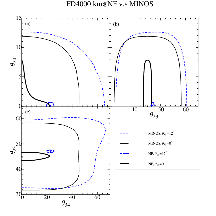

A similar analysis is performed in ??[61] by the MINOS collaboration. The mixing matrix parametrization in this reference is equivalent to ours since they fix their , corresponding to our , to zero. One of the schemes tested in ??[61] assumed that (in mass ordering A). We show their result for the combined fits in the – (a), – (b), and – (c) planes in Fig. 6. Note that the not shown parameters are fixed, such as and the phases, and that is fixed to two different values (not marginalized over). The best-fit values are also marked. We also show the results for the Neutrino Factory under the same assumptions, where we use the 4000 km baseline only. Obviously, the Neutrino Factory would reduce the allowed parameter space significantly, especially if is large. Again, note that some of the parameters are fixed here, and the full marginalization would destroy the sensitivities. The impact of additional near detectors, which are especially sensitive to , and an additional far detector at 7500 km, which is sensitive to , is shown in Fig. 7. Here the NF contours for large almost shrink to points, and are hardly visible anymore. In this figure, is assumed, and is not marginalized over. For such a value of , we would also expect a small effect in the MINOS near detector, which is, however, not considered in ??[61].
The special case
As similar kind of analysis can be performed in the special case , for which also no additional mass squared difference appears and . In this case, we have some sensitivity to in , as shown in the Appendix A. The comparison between MINOS and the Neutrino Factory is shown for this special case in Fig. 8, and again the Neutrino Factory has an excellent sensitivity. The marginalization over and the other parameters will, however, destroy the sensitivity to , since there is no sensitivity in Fig. 2 for . This is another good example that the set of assumptions determines the outcome, whereas the general analysis would simply produce no sensitivity.
Comparison to two-flavor limits
Especially for short-baseline new physics searches, in the literature often two baseline limits are discussed. That is, at a short baseline where no standard oscillations occur, sterile neutrinos are searched for using a two flavor fit. An example is the short-baseline electron neutrino disappearance considered in the two flavor limit:
| (22) |
In ??[54], even the test of CPT invariance at such a short baseline was considered. From our discussion in Sec. 2.2, it is clear that the short-baseline disappearance channels are the key measurements for the active-sterile-mixings, because they are uniquely sensitive to one parameter (or one mixing matrix element). On the other hand, the appearance channels, such as the tau neutrino appearance in NOMAD and CHORUS or the electron neutrino appearance in MiniBooNE, measure combinations of parameters. A signal in this channel would inevitably point towards new physics, but these channels are not very useful to limit individual active-sterile mixing parameters (or mixing matrix elements).
Eq. (22) can be directly related to our parametrization with the identification and . Correspondingly, the results of our analysis for are similar to ??[54] (see Fig. 3). On the other hand, it was emphasized in ??[54] that cross section measurements will spoil the disappearance measurements, and that these can be controlled with additional near detectors very close to the source. Since there is no CP violation in short-baseline disappearance measurements (neither from CP phases nor from the MSW effect), the disappearance channels can also be used for clean CPT invariance tests.
Note that a CPT invariance test of the MiniBooNE result would be, in principle, also possible at the Neutrino Factory, because both and could be tested. However, for these appearance channels electron charge identification is required to distinguish, for example, from the background. Therefore, the direct test of the recent anomaly [11] may be difficult.
5 Summary and conclusions
In this work, we have discussed sterile neutrinos beyond LSND, i.e., sterile neutrinos with small active-sterile mixings and an arbitrary . We have used the Neutrino Factory for the simulation, since this experiment can be used for a self-consistent approach including near and far detectors. We have used the simplest possible hypothesis, namely one extra sterile neutrino in a 3+1-like scheme in which the standard scenario is recovered for small active-sterile mixing angles. While we obtain the expected sensitivity to the active-sterile mixing in the large LSND-motivated region, we also find sensitivity close to the atmospheric . We have pointed out that there are no global fits for this case yet, and a re-analysis of atmospheric and solar data should demonstrate what we can learn for . Note that recent cosmological fits point towards one or two such light sterile neutrinos [12].
We have demonstrated that, especially at the short baselines, the disappearance channels are the primary channels of interest for light sterile neutrino constraints, no matter if a parametrization-independent approach or a particular parametrization for the mixing matrix is used. For the combined analysis of short and long baselines including charged and neutral current matter effects, however, we have used a particular parametrization. We have demonstrated that the most general constraint on sterile species can be shown as exclusion limits in the ––planes (, , ), similar to the CHOOZ limit for –. The Neutrino Factory turns out to have excellent sensitivity to the three mixing angles in a wide range of . However, one of the three mixing angles ( in our parametrization) can only be very well measured for large at the near detectors, and one ( in our parametrization) better for small , whereas the third () can be measured in the combined range. An electron neutrino disappearance channel at the long baselines could solve this problem for , which is, however, difficult at the Neutrino Factory, because electron charge identification might be required. An improved measurement of for large would require a hypothetical disappearance channel. We have also investigated the impact of different mass orderings (cf., Fig. 1) on the sensitivities. We have found that there is a qualitative difference between the cases and due to different matter effects. Furthermore, we have tested the impact of additional detectors with an aggressive 10 kt OPERA-like detector at the short and long baselines, and we have not found any significant effect on the sensitivities.
Apart from the general constraints, we have compared our analysis to special cases in the literature. For instance, we have tested the case leading to averaging of the fast oscillations at the long baselines. We have looked into the special case of a - fit. We have shown that this assumption involves subtleties, especially if additional near detectors are considered, because the assumption for implies that there may be effects in the near detectors. We have illustrated that in this case additional assumptions are required, and the interpretation of the sensitivities becomes strongly assumption-dependent. This does not apply to our general bounds we discussed above. We have also tested the impact of detection (“discovery channel”), and we could find a marginal improvement. The main sensitivity, however, comes from the muon neutrino disappearance channel for . We have moreover compared the Neutrino Factory to a recent MINOS analysis using the same assumptions, and we have found excellent sensitivities. However, including the full marginalization over the unknown parameters, the sensitivities were basically destroyed.
In conclusion, although the sensitivities of the Neutrino Factory to light sterile neutrinos in the atmospheric mass squared range may not be extremely compelling, these bounds are very robust and independent of any special assumptions. If special assumptions are used, such as often done in the literature, the sensitivities look extremely good. Of course our results are not the most general case, one could also study scenarios. However, even for the scenario, this analysis is extremely challenging because there can be interference between the known and the unknown mass squared differences. A re-analysis of atmospheric and solar experiments could provide clues on what one can learn already from existing experiments. Finally, even the test in supernovae may be interesting, because one may expect additional resonances or new (neutral current) matter effects.
Acknowledgments
We would like to thank Carlo Giunti and Marco Laveder for lively discussions during the first stages of this work, and Michele Maltoni for useful discussions. We would also like to thank Xiaobo Huang, Jiajie Ling, Anthony Mann, Brian Rebel, and Alexandre Sousa in the MINOS collaboration for help to make a direct comparison between their results and ours possible.
This work has been supported by the Emmy Noether program of Deutsche Forschungsgemeinschaft (DFG), contract no. WI 2639, by the DFG-funded Graduiertenkolleg 1147 “Theoretical astrophysics and particle physics” [J.T.], and by the European Union under the European Commission Framework Programme 07 Design Study EUROnu, Project 212372.
Appendix A in the limit
In this appendix we show the transition probability in the limit and . We study the explicit dependence on to all orders in perturbation theory, while keeping and all other mixing angles vanishing. We get:
where
| (24) |
We see that the dependence on (through the terms) appears in terms with different energy dependencies, which makes a spectral analysis at the Neutrino Factory useful to get a non-vanishing sensitivity even in the limit. Interestingly enough, the matter effects are driven by the neutral current potential , because of the vanishing approximation.
References
- [1] M. C. Gonzalez-Garcia and M. Maltoni, Phys. Rept. 460, 1 (2008), 0704.1800.
- [2] Y. Fukuda et al. (Super-Kamiokande), Phys. Rev. Lett. 81, 1562 (1998), hep-ex/9807003.
- [3] P. Adamson et al. (MINOS), Phys. Rev. Lett. 101, 131802 (2008), 0806.2237.
- [4] Q. R. Ahmad et al. (SNO), Phys. Rev. Lett. 89, 011301 (2002), nucl-ex/0204008.
- [5] T. Araki et al. (KamLAND), Phys. Rev. Lett. 94, 081801 (2005), hep-ex/0406035.
- [6] M. Apollonio et al. (CHOOZ), Eur. Phys. J. C27, 331 (2003), hep-ex/0301017.
- [7] G. L. Fogli, E. Lisi, A. Marrone, A. Palazzo, and A. M. Rotunno, Phys. Rev. Lett. 101, 141801 (2008), 0806.2649.
- [8] A. Aguilar et al. (LSND), Phys. Rev. D64, 112007 (2001), hep-ex/0104049.
- [9] M. Maltoni and T. Schwetz, Phys. Rev. D76, 093005 (2007), 0705.0107.
- [10] S. Palomares-Ruiz, S. Pascoli, and T. Schwetz, JHEP 09, 048 (2005), hep-ph/0505216.
- [11] A. A. Aguilar-Arevalo et al. (The MiniBooNE) (2010), 1007.1150.
- [12] J. Hamann, S. Hannestad, G. G. Raffelt, I. Tamborra, and Y. Y. Y. Wong (2010), 1006.5276.
- [13] M. Apollonio et al. (2002), hep-ph/0210192.
- [14] C. Albright et al. (Neutrino Factory/Muon Collider) (2004), physics/0411123.
- [15] A. Bandyopadhyay et al. (ISS Physics Working Group), Rept. Prog. Phys. 72, 106201 (2009), 0710.4947.
- [16] T. Abe et al. (ISS Detector Working Group), JINST 4, T05001 (2009), 0712.4129.
- [17] M. Apollonio et al. (ISS Accelerator Working Group), JINST 4, P07001 (2009), 0802.4023.
- [18] International design study of the neutrino factory, http://www.ids-nf.org.
- [19] P. Huber and W. Winter, Phys. Rev. D68, 037301 (2003), hep-ph/0301257.
- [20]
V. Barger,
S. Geer, and
K. Whisnant,
Phys. Rev. D61,
053004 (2000),
hep-ph/9906487. - [21] A. Cervera et al., Nucl. Phys. B579, 17 (2000), hep-ph/0002108.
- [22] J. Burguet-Castell, M. B. Gavela, J. J. Gomez-Cadenas, P. Hernandez, and O. Mena, Nucl. Phys. B608, 301 (2001), hep-ph/0103258.
- [23] M. Freund, P. Huber, and M. Lindner, Nucl. Phys. B615, 331 (2001), hep-ph/0105071.
- [24] A. Donini, E. Fernandez-Martinez, D. Meloni, and S. Rigolin, Nucl. Phys. B743, 41 (2006), hep-ph/0512038.
- [25] P. Huber, M. Lindner, M. Rolinec, and W. Winter, Phys. Rev. D74, 073003 (2006), hep-ph/0606119.
- [26] R. Gandhi and W. Winter, Phys. Rev. D75, 053002 (2007), hep-ph/0612158.
- [27] J. Kopp, T. Ota, and W. Winter, Phys. Rev. D78, 053007 (2008), 0804.2261.
- [28] J. Tang and W. Winter, Phys. Rev. D80, 053001 (2009), arXiv:0903.3039.
- [29] S. Geer, O. Mena, and S. Pascoli, Phys. Rev. D75, 093001 (2007), hep-ph/0701258.
- [30] A. D. Bross, M. Ellis, S. Geer, O. Mena, and S. Pascoli, Phys. Rev. D77, 093012 (2008), 0709.3889.
- [31] P. Huber and W. Winter, Phys. Lett. B655, 251 (2007), 0706.2862.
- [32] A. Bross et al., Phys. Rev. D81, 073010 (2010), 0911.3776.
- [33] E. Fernandez Martinez, T. Li, S. Pascoli, and O. Mena, Phys. Rev. D81, 073010 (2010).
- [34] J. Tang and W. Winter, Phys. Rev. D81, 033005 (2010), 0911.5052.
- [35] S. Antusch, C. Biggio, E. Fernandez-Martinez, M. B. Gavela, and J. Lopez-Pavon, JHEP 10, 084 (2006), hep-ph/0607020.
- [36] E. Fernandez-Martinez, M. B. Gavela, J. Lopez-Pavon, and O. Yasuda, Phys. Lett. B649, 427 (2007), hep-ph/0703098.
- [37] A. Abada, C. Biggio, F. Bonnet, M. B. Gavela, and T. Hambye, JHEP 12, 061 (2007), 0707.4058.
- [38] S. Goswami and T. Ota, Phys. Rev. D78, 033012 (2008), 0802.1434.
- [39] M. Malinsky, T. Ohlsson, and H. Zhang, Phys. Rev. D79, 073009 (2009), 0903.1961.
- [40] D. Meloni, T. Ohlsson, W. Winter, and H. Zhang, JHEP 04, 041 (2010), 0912.2735.
- [41] P. Huber, T. Schwetz, and J. W. F. Valle, Phys. Rev. D66, 013006 (2002), hep-ph/0202048.
- [42] N. C. Ribeiro, H. Minakata, H. Nunokawa, S. Uchinami, and R. Zukanovich-Funchal, JHEP 12, 002 (2007), 0709.1980.
- [43] S. Antusch, J. P. Baumann, and E. Fernandez-Martinez, Nucl. Phys. B810, 369 (2009), 0807.1003.
- [44] M. Blennow, D. Meloni, T. Ohlsson, F. Terranova, and M. Westerberg, Eur. Phys. J. C56, 529 (2008), 0804.2744.
- [45] T. Ohlsson and H. Zhang, Phys. Lett. B671, 99 (2009), 0809.4835.
- [46] M. Malinsky, T. Ohlsson, and H. Zhang, Phys. Rev. D79, 011301 (2009), 0811.3346.
- [47] M. B. Gavela, D. Hernandez, T. Ota, and W. Winter, Phys. Rev. D79, 013007 (2009), 0809.3451.
- [48] A. Donini, M. B. Gavela, P. Hernandez, and S. Rigolin, Nucl. Phys. B574, 23 (2000), hep-ph/9909254.
- [49] A. Kalliomaki, J. Maalampi, and M. Tanimoto, Phys. Lett. B469, 179 (1999), hep-ph/9909301.
- [50] A. Donini, M. Lusignoli, and D. Meloni, Nucl. Phys. B624, 405 (2002), hep-ph/0107231.
- [51] A. Donini and D. Meloni, Eur. Phys. J. C22, 179 (2001), hep-ph/0105089.
- [52] A. Dighe and S. Ray, Phys. Rev. D76, 113001 (2007), 0709.0383.
- [53] A. Donini, K.-i. Fuki, J. Lopez-Pavon, D. Meloni, and O. Yasuda, JHEP 08, 041 (2009), 0812.3703.
- [54] C. Giunti, M. Laveder, and W. Winter, Phys. Rev. D80, 073005 (2009), 0907.5487.
- [55] O. Yasuda (2010), 1004.2388.
- [56] M. Maltoni, T. Schwetz, M. A. Tortola, and J. W. F. Valle, Phys. Rev. D67, 013011 (2003), hep-ph/0207227.
- [57] M. Maltoni, T. Schwetz, M. A. Tortola, and J. W. F. Valle, New J. Phys. 6, 122 (2004), hep-ph/0405172.
- [58] P. Astier et al. (NOMAD), Nucl. Phys. B611, 3 (2001), hep-ex/0106102.
- [59] E. Eskut et al. (CHORUS), Nucl. Phys. B793, 326 (2008), 0710.3361.
- [60] A. Donini, M. Maltoni, D. Meloni, P. Migliozzi, and F. Terranova, JHEP 12, 013 (2007), 0704.0388.
- [61] P. Adamson et al. (The MINOS), Phys. Rev. D81, 052004 (2010), 1001.0336.
- [62] C. Giunti and C. W. Kim Oxford, UK: Univ. Pr. (2007) 710 p.
- [63] P. Huber, M. Lindner, and W. Winter, Comput. Phys. Commun. 167, 195 (2005), http://www.mpi-hd.mpg.de/lin/globes/, hep-ph/0407333.
- [64] P. Huber, J. Kopp, M. Lindner, M. Rolinec, and W. Winter, Comput. Phys. Commun. 177, 432 (2007), hep-ph/0701187.
- [65] J. Kopp, Int. J. Mod. Phys. C19, 523 (2008), physics/0610206.
- [66] M. Blennow and E. Fernandez-Martinez, Comput. Phys. Commun. 181, 227 (2010), 0903.3985.
- [67] P. Huber, M. Lindner, and W. Winter, Nucl. Phys. B645, 3 (2002), hep-ph/0204352.
- [68] E. Ables et al. (MINOS) FERMILAB-PROPOSAL-P-875.
- [69] D. Autiero et al., Eur. Phys. J. C33, 243 (2004), hep-ph/0305185.
- [70] M. C. Gonzalez-Garcia, M. Maltoni, and J. Salvado, JHEP 04, 056 (2010), 1001.4524.
- [71] R. J. Geller and T. Hara, Phys. Rev. Lett. 49, 98 (2001), hep-ph/0111342.
- [72] T. Ohlsson and W. Winter, Phys. Rev. D68, 073007 (2003), hep-ph/0307178.