Combining DFT and Many-Body Methods to Understand Correlated Materials

In the projector-operator method, each (nonorthonormalized) Wannier function is generated by projecting a trial basis function $|\tilde{\chi}_{{\bf R}}^{t}\rangle$, centered at the site ${\bf R}$, onto the $L$-bands:

where

is the projector-operator onto the $L$-bands, $\psi_{i}$ is the eigenstate of $\hat{H}$, and $i$ is a joint index combining the band index and the position of the momentum ${\bf k}$ in the first Brillouin zone. The functions $\{W_{{\bf R}}^{t}\}$ can be numerically orthonormalized,

where $\hat{\cal S}$$=$$\|{\cal S}_{{\bf R}^{\prime}{\bf R}}^{t^{\prime}t}\|$ is the overlap matrix,

Then, the one-electron part of the model Hamiltonian (3) is defined by the matrix elements of $\hat{H}$ in the basis of these orthonormalized Wannier orbitals:

The conventional downfolding method also implies that the atomic basis can be divided into two parts: $\{\tilde{\chi}_{\bf R}\}$$=$$\{\tilde{\chi}_{\bf R}^{t}\}$$\oplus$$\{\tilde{\chi}_{\bf R}^{r}\}$, so that the low-energy part of the spectrum is mainly represented by the $\{\tilde{\chi}_{\bf R}^{t}\}$-states, while $\{\tilde{\chi}_{\bf R}^{r}\}$ is the rest of the basis states, which mainly contribute to the higher-energy part. Then, each eigenstate of $\hat{H}$ can be identically presented as the sum $|\psi_{i}\rangle$$=$$|\psi_{i}^{t}\rangle$$+$$|\psi_{i}^{r}\rangle$, where $|\psi_{i}^{t}\rangle$ and $|\psi_{i}^{r}\rangle$ are expanded over the basis states of the “$t$” and “$r$” types, respectively. In this case, the Schrödinger equation for $|\psi_{i}\rangle$ takes the following form:

where $\hat{H}^{t(r)t(r)}$ are the blocks of matrix elements of $\hat{H}$ in the basis of “$t$”(“$r$”)-states. The effective $\omega$-dependent Hamiltonian $\hat{H}_{\rm eff}$ is obtained by expressing $|\psi_{i}^{r}\rangle$ from (10),

and substituting into (9). This yields

which formally acts only on $|\psi_{i}^{t}\rangle$. However, $|\psi_{i}^{t}\rangle$ is only a part of the eigenvector, which is not orthonormalized. Therefore, $\hat{H}_{\rm eff}(\omega)$ should be additionally transformed to an orthonormal representation:

which is specified by the overlap matrix,

The latter is obtained after the substitution of (11) into the normalization condition: $\langle\psi_{i}^{t}|\psi_{i}^{t}\rangle$$+$$\langle\psi_{i}^{r}|\psi_{i}^{r}\rangle$$=$$1$.

In the conventional downfolding method, $\hat{h}$ is typically evaluated in the center of gravity of the $L$-bands, $\omega_{0}$. Although the downfolding method does not explicitly require the construction of the Wannier functions, they can be formally reconstructed from $\hat{h}(\omega_{0})$ [22].

The conventional downfolding method is exact. However, this property is guaranteed by the $\omega$-dependence of $\hat{h}$, which is hardly useful from the practical point of view. Formally, for each $\psi_{i}$, $\omega$ in (13) should coincide with the eigenvalue of $\hat{H}$ corresponding to this $\psi_{i}$. Moreover, $\hat{h}(\omega)$ retains an excessive information about $\hat{H}$, so that the full spectrum of $\hat{H}$ can be formally derived from $\hat{h}(\omega)$. However, typically we do not need such a redundant information and would like to use $\hat{h}$ only for a small group of electronic states located near the Fermi level, and do it in the most exact form.

For these purposes, the downfolding method can be reformulated as a projector-operator method and reduced to it [23]. The trick is to replace the original Hamiltonian $\hat{H}$ in the downfolding method by a modified Hamiltonian $\hat{H}^{\prime}$, which has the same set of eigenvalues $\{\varepsilon_{i}\}$ and eigenfunctions $\{\psi_{i}\}$ in the region of $L$-bands.³³ 3 This procedure was already used in [5, 20, 21, 22]. However, the details have been explained only in [23]. The rest of the eigenstates is not important for the construction of the one-electron part of the model Hamiltonian and can be placed to the region of infinite energies. Hence, we define $\hat{H}^{\prime}$ in the following form:

where $\hat{P}_{\perp}$$=$$\hat{1}$$-$$\hat{P}$ is the projector operator to the subspace orthogonal to the $L$-bands and $\epsilon$$\rightarrow$$\infty$. According to the choice of the basis functions $\{\tilde{\chi}_{\bf R}^{t}\}$ and $\{\tilde{\chi}_{\bf R}^{r}\}$ in the downfolding method, the latter mainly contribute to the high-energy part of the spectrum. Therefore, the overlap between $\psi_{i}$ in the low-energy part and any of $\{\tilde{\chi}_{\bf R}^{r}\}$ should be small, so that all eigenvalues of $(\hat{H}^{\prime})^{rr}$ are of the order of $\epsilon$. Then, it is intuitively clear that in the limit $\epsilon$$\to$$\infty$, the $\omega$-dependence in (11) will disappear and the method will be exact. This statement can be proven rigorously, and such a proof can be found in [23].

Thus, by introducing the modified Hamiltonian of the form (15), the downfolding method can be naturally reformulated as the projector-operator method. The advantage of this procedure is that it allows us to go directly to the construction of the one-electron Hamiltonian $\hat{h}$, and formally skip the step of the construction of the Wannier functions.

Finally, we would like to note that (15) is nothing but a scissor-operator-like transformation of the original Hamiltonian $\hat{H}$, and this strategy is different from the order-$N$ muffin-tin orbital method, which was also used for the construction of the Wannier functions and where the basic idea was to make some approximations for the $\omega$-dependence of the downfolded Hamiltonian [24].

At the beginning of this section we have argued that the basis functions $\{\tilde{\chi}_{\bf R}^{\alpha}\}$ can be regarded as the Wannier functions of the full Hamiltonian $\hat{H}$. Now, let us assume that each basis function is localized around the central atomic site and satisfies certain criteria of the “maximal localization”, such that any linear combination of $\{\tilde{\chi}_{\bf R}^{\alpha}\}$ will be “less localized” in comparison with the basis function $\tilde{\chi}_{\bf R}^{\alpha}$ from the original basis set, or at least has the same degree of the localization, if we are dealing with the linear combination of orbitals centered at the same atomic site.⁴⁴ 4 The precise criterion of the maximal localization is not really important at this stage, because this is merely a mathematical construction and depending on the considered physical property one can introduce different criteria of the “maximal localization”. However, this is not necessarily true if one wants to construct the Wannier functions only for some part of the electronic structure, which is specified by the subspace $L$ of the full Hamiltonian $\hat{H}$. Due to the additional orthogonality condition to other bands, such a Wannier function will inevitably be a linear combination of $\{\tilde{\chi}_{\bf R}^{\alpha}\}$. Therefore, it will inevitably be less localized in comparison with the trial function $\tilde{\chi}_{\bf R}^{t}$.

Nevertheless, one can try to “minimize” the deviation from the original formulation for the full Hamiltonian $\hat{H}$ and ask which single atomic orbital centered at the site ${\bf R}$ will be the best representation for the Wannier orbital. Therefore, we search a new set of trial functions in the form:

and find the coefficients $\{c_{\bf R}^{\alpha}\}$, which maximize the projection $\langle\tilde{\phi}^{t}_{\bf R}|W^{t}_{\bf R}[\tilde{\phi}^{t}_{\bf R}]\rangle$ of $\tilde{\phi}^{t}_{\bf R}$ onto the nonorthonormalized Wannier function constructed from $\tilde{\phi}^{t}_{\bf R}$ using the projector-operator technique, $|W^{t}_{\bf R}[\tilde{\phi}^{t}_{\bf R}]\rangle$$=$$\hat{P}|\tilde{\phi}^{t}_{\bf R}\rangle$. It will automatically guarantee that $\tilde{\phi}^{t}_{\bf R}$ is the best single-orbital representation for $W^{t}_{\bf R}$ in the projector-operator method among the trial orbitals of the form (16). By substituting $W^{t}_{\bf R}[\tilde{\phi}^{t}_{\bf R}]$ into the projection $\langle\tilde{\phi}^{t}_{\bf R}|W^{t}_{\bf R}[\tilde{\phi}^{t}_{\bf R}]\rangle$, problem is reduced to the maximization of

with respect to $\{c_{\bf R}^{\alpha}\}$, where the Lagrange multipliers $\{\lambda\}$ enforce the orthonormality condition for $\{\tilde{\phi}^{t}_{\bf R}\}$. Then, the maximization of $D$ is equivalent to the diagonalization of $\hat{P}_{\bf RR}$$=$$\|\langle\tilde{\chi}_{\bf R}^{\alpha}|\hat{P}|\tilde{\chi}_{\bf R}^{\alpha^{\prime}}\rangle\|$, which is nothing but the site-diagonal part of the density matrix constructed from the $L$-bands in the basis of atomic orbitals $\{\tilde{\chi}_{\bf R}^{\alpha}\}$. After the diagonalization, we should simply pick up $n$ eigenstates $\{\tilde{\phi}^{t}_{\bf R}\}$, corresponding to maximal eigenvalues $\{\lambda\}$, where $n$ is the number of Wannier functions centered at the atomic site ${\bf R}$.⁵⁵ 5 This can be paraphrased in a different way [5]. Of course, any set of the Wannier functions should be able to reproduce the total density at the site ${\bf R}$. Each Wannier function consists of the central part (or “head”), located at the site ${\bf R}$, and the tail, spreading over the other sites. By identifying $\{\tilde{\phi}^{t}_{\bf R}\}$ with eigenstates corresponding to the maximal eigenvalues of the density matrix $\{\lambda\}$, we guarantee that the main part of the density at the site ${\bf R}$ is described by the “heads” of the Wannier functions. Then, the remaining part of the density, corresponding to other (small) $\{\lambda\}$, is described by the tails of the Wannier functions coming from other sites. This implies that the weights of these tails should be also small. These $\{\tilde{\phi}^{t}_{\bf R}\}$ will maximize $D$. This procedure has been proposed in [20] without any proof. Then, some intuitive arguments have been given in [22]. The rigorous proof has been given in [23].

Electronic structure calculations are typically supplemented with some additional approximations, like the atomic-sphere-approximation (ASA), where the LDA potential is spherically averaged inside certain atomic spheres [13]. If ASA is used in the process of construction of the model Hamiltonian, the parameters $\{h_{{\bf R}{\bf R}^{\prime}}^{\alpha\beta}\}$ will include all effects of the covalent mixing effects between atomic orbitals. However, there will be other effects, which are not accounted by $\{h_{{\bf R}{\bf R}^{\prime}}^{\alpha\beta}\}$. The most important contribution comes from the nonsphericity (n-s) of the Madelung potential for the electron-ion interactions, which contributes to the crystal-field splitting [25].⁶⁶ 6 In fact, the contribution of Coulomb interactions to the crystal-field splitting is a tricky issue. Despite an apparent simplicity of the problem, one should clearly distinguish different contributions and not to include them twice, for example, to the one-electron and Coulomb interaction parts of the model Hamiltonian (3). In this sense, the use of full-potential techniques does not automatically guarantee the right answer. Note that the nonsphericity of on-site interactions is explicitly included into the second part of the model Hamiltonian (3). Therefore, in order to not to include it twice, one should subtract the corresponding contributions to the one-electron part originating from the Coulomb and exchange-correlation potentials in LDA. The proper correction to $\|h_{{\bf R}{\bf R}^{\prime}}^{\alpha\beta}\|$ can be computed in the Wannier basis as:

where $Z^{*}_{{\bf R}^{\prime}}$ is the total charge associated with the site ${\bf R}^{\prime}$ (namely, the nuclear charge minus the screening electronic charge encircled by the atomic sphere), and ${\bf r}$ is the position of electron in the sphere ${\bf R}$.

The main idea behind this treatment is based on certain hierarchy of interactions in solids. It implies that the strongest interaction, which leads to the energetic separation of the $L$-band from other bands (Figure 1), is due to the covalent mixing. For example, in many transition-metal oxides this interaction is responsible for the famous splitting between transition-metal $t_{2g}$ and $e_{g}$ bands [26]. The nonsphericity of the Madelung potential is considerably weaker than this splitting. However, it can be comparable with the covalent mixing in the narrow $L$-band. Therefore, the basic idea is to treat this nonsphericity as a pseudo-perturbation [13], and calculate the matrix elements of the Madelung potential in the basis of Wannier functions constructed for spherically averaged ASA potential.

The same strategy can be applied to the spin-orbit (s-o) interaction, which yields the following correction to $\|h_{\bf RR}^{\alpha\beta}\|$:

Here, $V$ is the self-consistent LDA potential and $\boldsymbol{\sigma}$ is the vector of Pauli matrices.

The dependence of the total energy $E[\{n_{{\bf R}\alpha}\}]$ on the individual occupation numbers $\{n_{{\bf R}\alpha}\}$ can be obtained by applying the constrained density-functional theory [29, 30, 31, 32]:

where $\hat{\rho}({\bf r},{\bf r}^{\prime})=\sum_{i}f_{i}\psi_{i}^{\dagger}({\bf r})\psi_{i}({\bf r}^{\prime})$ is the density operator constructed from the Kohn-Sham orbitals, $\rho({\bf r})=\hat{\rho}({\bf r},{\bf r})$ is the electron density, and $\{V_{{\bf R}\alpha}\}$ are the external potentials, which play the role of Lagrange multipliers and enforce the occupations of the Wannier orbitals to be equal to $\{n_{{\bf R}\alpha}\}$. As it was already pointed out in the Introduction, in spite of many limitations for the strongly correlated systems, LDA is formulated as an approximation to the theory of the ground-state. Therefore, there is always a hope that it will provide a good estimate for $U_{\alpha\alpha\beta\beta}$ as long as the latter is expressed in terms of the total energy difference (18) or any other quantity, which is uniquely related with this total energy difference.

The total energy difference (18) is typically replaced by the difference of Kohn-Sham eigenvalues $\{\varepsilon_{{\bf R}\alpha}\}$ calculated for an intermediate configuration, by using Slater’s transition state arguments:⁸⁸ 8 Here, we also use the reciprocity condition $\varepsilon_{{\bf R}^{\prime}\beta}[n_{{\bf R}\alpha}$$+$$\frac{1}{2},n_{{\bf R}^{\prime}\beta}$$-$$\frac{1}{2}]=\varepsilon_{{\bf R}\alpha}[n_{{\bf R}\alpha}$$-$$\frac{1}{2},n_{{\bf R}^{\prime}\beta}$$+$$\frac{1}{2}]$ for two fluctuations around the uniform state with $n_{{\bf R}\alpha}=n_{{\bf R}^{\prime}\beta}$.

It implies the validity of Janak’s theorem [33]

However, in order to use this theorem, $\{\tilde{W}_{\bf R}^{\alpha}\}$ must be the eigenvectors of Kohn-Sham equations (1). Otherwise, Janak’s theorem is not applicable, and the eigenvalues $\{\varepsilon_{{\bf R}\alpha}\}$ are ill-defined.⁹⁹ 9 For example, by defining $\varepsilon_{{\bf R}\alpha}$ as the diagonal matrix element of the Kohn-Sham Hamiltonian $\hat{H}$, $\varepsilon_{{\bf R}\alpha}$$=$$\langle\tilde{W}_{\bf R}^{\alpha}|\hat{H}|\tilde{W}_{\bf R}^{\alpha}\rangle$, does not necessary guarantee that this $\varepsilon_{{\bf R}\alpha}$ is equal to $\partial E/n_{{\bf R}\alpha}$, and (20) is consistent with the more general definition (18). Of course, this assumption does not work for the regular Wannier functions $\{\tilde{W}_{\bf R}^{\alpha}\}$ constructed for the LDA Hamiltonian $\hat{H}$.¹⁰¹⁰ 10 Note that if $\{\tilde{W}_{\bf R}^{\alpha}\}$ were the eigenvectors of $\hat{H}$, all transfer integrals, which are defined as off-diagonal matrix elements of $\hat{H}$ with respect to $\tilde{W}_{\bf R}^{\alpha}$ and $\tilde{W}_{{\bf R}^{\prime}}^{\beta}$ would vanish (see Section 3.1).

Nevertheless, there is a transparent and physical solution of this problem, which rehabilitates the use of Janak’s theorem. Indeed, since the kinetic-energy term is explicitly included into the Hubbard model (3), it should not contribute to the total energy difference (18). Otherwise, it would be included twice, and we would face the problem of the double counting [30, 31]. This can be done by artificially switching off all matrix elements of $\hat{H}$ between $\tilde{W}_{\bf R}^{\alpha}$ and $\tilde{W}_{{\bf R}^{\prime}}^{\beta}$, which is equivalent to switching off the transfer integrals. Another solution is to modify the Wannier functions $\{\tilde{W}_{\bf R}^{\alpha}\}\rightarrow\{\bar{W}_{\bf R}^{\alpha}\}$ (apparently by considering another boundary conditions) in order to enforce the property $\langle\bar{W}_{\bf R}^{\alpha}|\hat{H}|\bar{W}_{{\bf R}^{\prime}}^{\beta}\rangle$$=$$0$ for the given LDA Hamiltonian $\hat{H}$ [22].¹¹¹¹ 11 This can be naturally done by reconstructing the Wannier functions from the matrix elements $h_{{\bf RR}^{\prime}}^{\alpha\beta}$ derived from the downfolded method [22]. Nevertheless, it seems that for many strongly correlated systems, $\{\bar{W}_{\bf R}^{\alpha}\}$ do not substantially differ from $\{\tilde{W}_{\bf R}^{\alpha}\}$. The intuitive reason for that is that the transfer integrals in the narrow $L$-band are typically much smaller in comparison with other effects of the covalent mixing, which lead to the separation of the $L$-band from other bands and mainly determine the shape of the Wannier functions. Another reason is that for strongly correlated systems, the transfer integrals are typically much smaller than the on-site Coulomb interactions. Therefore, to certain extent it is unimportant whether the small transfer integrals are included in the definition of the large Coulomb interactions or not as they cause only small change of these interactions. These $\{\bar{W}_{\bf R}^{\alpha}\}$ can be regarded as the eigenfunctions of $\hat{H}$, that justifies the use of Janak’s theorem.

Finally, in the first order of $\pm$$\frac{1}{2}$, (20) can be transformed to

where the derivative is calculated under the condition that the total number of electrons is conserved: $n_{{\bf R}\alpha}$$+$$n_{{\bf R}^{\prime}\beta}$$=$${\rm const}$.

It is important that in the process of solution of the Kohn-Sham equations, the Wannier orbitals (and all remaining electronic structure) are allowed to relax in order to to adjust the change of the occupation numbers $\{n_{{\bf R}\alpha}\}$. This relaxation is an important channel of screening. As we shall see below, the values of the screened Coulomb interactions in the $L$-band are defined not only by the extension of the Wannier functions in the ground state, but mainly by the change of these functions during the reaction ($n_{{\bf R}\alpha}$,$n_{{\bf R}^{\prime}\beta}$) $\rightleftharpoons$ ($n_{{\bf R}\alpha}$$+$$1$,$n_{{\bf R}^{\prime}\beta}$$-$$1$). Thus, in order to calculate $\hat{U}$, it is not sufficient to know the Wannier functions in the ground state. Even more important question is how these Wannier functions will be modified in the process of transfer of an electron from one site of the system to another.

Another way of calculating the screened Coulomb interaction is to use the random-phase approximation (RPA), which constitutes the basis of the GW method [34, 35, 37]. In this case, the effective Coulomb interaction is calculated in terms of the response onto the external perturbation of the electron density, $\delta\rho_{\rm ext}({\bf r})$, which is introduced as a probe of the electron system. RPA has many similarities with the constrained DFT. It consists of the following steps.

1. 1.

   $\delta\rho_{\rm ext}({\bf r})$ creates the Coulomb potential $\delta V_{\rm ext}({\bf r})=e^{2}\int d{\bf r}^{\prime}|{\bf r}$$-$${\bf r}^{\prime}|^{-1}\delta\rho_{\rm ext}({\bf r}^{\prime})$, which is similar to $\{V_{{\bf R}\alpha}\}$ in the constrained DFT, and $\delta\rho_{\rm ext}({\bf r})$ itself has a meaning of the electron density, which is controlled by the orbital occupations $\{n_{{\bf R}\alpha}\}$.¹²¹² 12 Yet, there is also a difference: $\delta V_{\rm ext}({\bf r})$ is the local potential, whereas $\{V_{{\bf R}\alpha}\}$ act on the individual Wannier functions $\{\tilde{W}_{\bf R}^{\alpha}\}$. This corresponds to the external potential $\delta V_{\rm ext}({\bf r},{\bf r}^{\prime})=\sum_{{\bf R}\alpha}V_{{\bf R}\alpha}|\tilde{W}_{\bf R}^{\alpha}\rangle\langle\tilde{W}_{\bf R}^{\alpha}|$ in the form of the projector operators, which are essentially nonlocal. This is the one of the basic differences between constrained DFT and RPA. The role of this nonlocality in the screening of the Coulomb interactions is not fully understood [38]. In principle, the perturbation of the electron density can also depend on time, that would correspond to the time-dependent DFT [36, 37]. Although such an extension can be certainly done, we will consider only the static (or time-independent) limit, strictly following the definition (18).

2. 2.

   $\delta V_{\rm ext}({\bf r})$ is treated as a perturbation. Then, the updates for the Kohn-Sham orbitals, $\{\delta\psi_{i}\}$, can be easily calculated in the first order of $\delta V_{\rm ext}({\bf r})$, by using the regular perturbation theory. The screening of the Coulomb interaction in RPA is entirely related with the change of $\{\psi_{i}\}$ or, in the other words, the relaxation of the Kohn-Sham orbitals.

3. 3.

   The change of the electron density is calculated from $\{\delta\psi_{i}\}$ in the first order of $\delta V_{\rm ext}({\bf r})$, namely, $\delta\rho({\bf r})=\sum_{i}[\delta\psi_{i}^{\dagger}({\bf r})\psi_{i}({\bf r})+\psi_{i}^{\dagger}({\bf r})\delta\psi_{i}({\bf r})]$.

4. 4.

   $\delta\rho({\bf r})$ results in the additional change of the Coulomb potential, also in the first order of $\delta V_{\rm ext}({\bf r})$: $\delta V_{\rm H}({\bf r})=e^{2}\int d{\bf r}^{\prime}|{\bf r}$$-$${\bf r}^{\prime}|^{-1}\delta\rho({\bf r}^{\prime})$.

5. 5.

   The steps (ii)-(iv) are repeated for the new potential, $\delta V_{\rm ext}({\bf r})$$+$$\delta V_{\rm H}({\bf r})$. Then, the potential is updated again, and so on. This is equivalent to the iterative solution of the Kohn-Sham equations within DFT. The constrained DFT also takes into account the change of the exchange-correlation potential, $V_{\rm XC}({\bf r})$. However, this change is typically treated in LDA, where the effect is small.

6. 6.

   After summing up an infinite number of updates for $\delta V_{\rm H}({\bf r})$, the screened Coulomb interaction in RPA is defined as $U({\bf r},{\bf r}^{\prime})=\delta V_{\rm ext}({\bf r})/\delta\rho_{\rm ext}({\bf r}^{\prime})+\delta V_{\rm H}({\bf r})/\delta\rho_{\rm ext}({\bf r}^{\prime})$.

Then, one can easily to show that $U({\bf r},{\bf r}^{\prime})$ satisfies the Dyson equation [34, 35]:

where ${\cal P}({\bf r},{\bf r}^{\prime})$ is the polarization function, which is obtained from the first-order perturbation theory expansion for $\{\delta\psi_{i}\}$:

The $\omega$-dependence of ${\cal P}({\bf r},{\bf r}^{\prime},\omega)$ corresponds to the time-dependent perturbation $\delta v_{\rm ext}({\bf r})\exp(-i\omega t)$. The static limit corresponds to ${\cal P}({\bf r},{\bf r}^{\prime},0)\equiv{\cal P}({\bf r},{\bf r}^{\prime})$. The prefactor “2” stands for two spin channels in the case of non-spin-polarized LDA.

The screened Coulomb interactions in RPA satisfies one very important property [39], which directly follows from the Dyson equation (23). Suppose that one can identify two different channels of screening, by dividing the full polarization function (24) into two parts: ${\cal P}={\cal P}_{1}+{\cal P}_{2}$. Then, the screened Coulomb interaction $U$ can be computed in two steps.

1. 1.

   By replacing total ${\cal P}$ by ${\cal P}_{1}$ in (23), one can compute the effective interaction $U_{1}$, which takes into account only the first channel of screening.

2. 2.

   Then, the final interaction $U$, corresponding to ${\cal P}_{1}$$+$${\cal P}_{2}$, can be obtained from $U_{1}$ again by using the Dyson equation (23), but where the full polarization function is replaced by ${\cal P}_{2}$:

   $$U({\bf r},{\bf r}^{\prime})=U_{1}({\bf r},{\bf r}^{\prime})+\int d{\bf r}^{\prime\prime}\int d{\bf r}^{\prime\prime\prime}U_{1}({\bf r},{\bf r}^{\prime\prime}){\cal P}_{2}({\bf r}^{\prime\prime},{\bf r}^{\prime\prime\prime})U({\bf r}^{\prime\prime\prime},{\bf r}^{\prime}).$$

This property has two important consequences.

1. 1.

   In order to calculate $U$, we would like to start with the LDA band structure. However, for Mott insulators, LDA yields an incorrect metallic behavior in the region of $L$-bands. Therefore, we should get rid of this unphysical metallic screening, which will always appear in RPA if one starts from LDA. More generally, RPA may not be a good approximation for treating the electron correlations in the narrow $L$-bands. Therefore, the general strategy is to get rid of the RPA self-screening associated with all kind of transitions between $L$-bands in the polarization function (24), and to replace it by a more rigorous model of screening in the process of solution of the Hubbard model (3) [21, 39]. The suppression of the transitions between $L$-bands in RPA is similar to switching off all transfer integrals between Wannier functions in the constrained DFT [22].¹³¹³ 13 Indeed, suppose that we have replaced $\{\psi_{i}\}$ for the $L$-bands in (24) by the Wannier functions $\{\tilde{W}_{\bf R}^{\alpha}\}$, and switched off all transfer integrals. In the ground state of such an auxiliary system, all occupation numbers are equal, $f_{i}$$=$$f_{j}$. Therefore, the polarization function (24) will vanish.

2. 2.

   Our goal is to evaluate the screening of the Coulomb interactions associated with the relaxation of the Wannier functions $\{\tilde{W}_{\bf R}^{\alpha}\}$ in the region of $L$-bands as well as of all other Kohn-Sham orbitals $\{\psi_{i}\}$ in the remaining part of the spectrum. Suppose that we are working in a (flexible) basis of atomic orbitals $\{\tilde{\chi}_{\bf R}^{\alpha}\}$, and both $\{\tilde{W}_{\bf R}^{\alpha}\}$ and $\{\psi_{i}\}$ are expanded over this basis:

   $$\left\{\begin{array}[]{c}\tilde{W}_{\bf R}^{\alpha}\\ \psi_{i}\\ \end{array}\right\}=\sum_{{\bf R}^{\prime}\beta}c_{{\bf R}^{\prime}}^{\beta}\tilde{\chi}_{{\bf R}^{\prime}}^{\beta}.$$

   (25)

   Then, within linear response theory, the relaxation of $\{\tilde{W}_{\bf R}^{\alpha}\}$ and $\{\psi_{i}\}$ will consist of two parts: the relaxation of the basis functions $\{\tilde{\chi}_{\bf R}^{\alpha}\}$ and the relaxation of the coefficients $\{c_{\bf R}^{\alpha}\}$ of the expansion over these basis functions, which corresponds to the change of the hybridization in the process of screening. Therefore, it has been proposed (though somewhat heuristically) that the screened Coulomb interactions in the $L$-band can be computed in two steps [22, 38]. For the sake of clarity, let us assume the main contribution to the $L$-bands comes from the $3d$ orbitals of the transition-metal sites.

   1. (a)

      The first step takes into account the screening caused by the relaxation of the basis functions $\{\tilde{\chi}_{\bf R}^{\alpha}\}$. It can be easily evaluated in the framework of constrained DFT. In this case, the Kohn-Sham equations are solved numerically on a finite grid of points in the real space, and $\{n_{{\bf R}\alpha}\}$ are the constrained $3d$ occupation numbers inside certain atomic spheres [29]. On the other hand, since RPA is based on the perturbation theory expansion, similar calculations in terms of the polarization function (24) would require an enormous number of states $\{\psi_{i}\}$, both in the occupied and unoccupied parts of the spectrum. Probably, this is one of the reasons why the conventional RPA calculations converge very slowly with the increase of the number of bands in the unoccupied part of the spectrum [40], and are extremely sensitive to the treatment of the core states [35]. The screening caused by the relaxation of the Kohn-Sham orbitals $\{\psi_{i}\}$ in the subspace orthogonal to $L$ (for example, the screening of localized $3d$ electrons by outer electrons in the transition-metal compounds) can be also easily taken into account in the conventional constrained DFT calculations [30, 31, 32].

   2. (b)

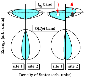
      However, what the constrained DFT cannot do is to treat the screening of Coulomb interactions amongst $3d$ electrons by the same $3d$ electrons [38, 41].¹⁴¹⁴ 14 The procedure implies that the atomic $3d$ charges can be divided into two parts, where the first part is subjected to the constraint conditions, while the second part is allowed to participate in the screening. Although, it can be formally done within constrained DFT [42], the actual computational scheme is rather laborious, and in many cases the procedure of dividing the atomic charges into the “screened” and “screening” parts is not well defined. Since the atomic $3d$ occupation numbers are rigidly fixed by the constraint conditions, the $3d$ electrons from other sites of the system cannot compensate the change of the number of the $3d$ electrons at the central site, and vise versa. However, such a channel of screening may exist. Suppose that our $L$-band is mainly constructed from the transition-metal $3d$ orbitals (the concrete example is the $t_{2g}$ band in the transition-metal oxides), and there is another, say oxygen $2p$ band, which has an appreciable weight of the atomic $3d$ orbitals (of both $t_{2g}$ and $e_{g}$ symmetry) coming from the hybridization between oxygen and transition-metal sites (Figure 2). Furthermore, the redistribution of the electron density in the $t_{2g}$ band, associated with the reaction ($n_{{\bf R}\alpha}$,$n_{{\bf R}^{\prime}\beta}$)$\rightleftharpoons$($n_{{\bf R}\alpha}$$+$$1$,$n_{{\bf R}^{\prime}\beta}$$-$$1$), will change the Coulomb potential around each transition-metal site. If the number of $t_{2g}$ electrons is increased by the constraint conditions, the Coulomb potential becomes more repulsive and vise versa. The more repulsive Coulomb potential will additionally push the $3d$ states from the oxygen $2p$ band to the higher-energy part of the spectrum. Therefore, around certain transition-metal sites, the change of the number of $3d$ electrons in the $t_{2g}$ band will be partly compensated by the change of the $3d$-electron density in the region of oxygen $2p$ band. This channel of screening can be easily evaluated in RPA, by rewriting (23) in the matrix form

      $$\hat{U}=\left[1-\hat{u}\hat{\cal P}\right]^{-1}\hat{u},$$

      (26)

      and assuming that all other channels of screening are already included in the definition the “bare Coulomb interaction” $\hat{u}$, derived from the constrained DFT [22]. Since the polarization matrix $\hat{\cal P}$ in (26) is aimed to describe the self-screening of the $3d$ electrons, it should consist of the matrix elements of (24) in the basis of atomic $3d$ orbitals, after the subtraction of the unphysical metallic screening associated with RPA transitions between $t_{2g}$ band.

The Hartree-Fock method provides the simplest approximation to the many-body problem (3). In this case, the trial many-electron wavefunction is searched in the form of a single Slater determinant $|S\{\varphi_{k}\}\rangle$, constructed from the one-electron orbitals $\{\varphi_{k}\}$. In this notation, $k$ is a collective index combining the momentum ${\bf k}$ of the first Brillouin zone, the band number, and the spin ($s$$=$ $\uparrow$ or $\downarrow$) of the particle. The one-electron orbitals are subjected to the variational principle and requested to minimize the total energy

for a given number of particles $\cal{N}$. This minimization is equivalent to the solution of Hartree-Fock equations for $\{\varphi_{k}\}$:

where $\hat{h}_{\bf k}$$\equiv$$\|h_{\bf k}^{\alpha\beta}\|$ is the one-electron part of the model Hamiltonian (3) in the reciprocal space, $h_{\bf k}^{\alpha\beta}$$=$$\sum_{{\bf R}^{\prime}}h^{\alpha\beta}_{{\bf R}{\bf R}^{\prime}}e^{-i{\bf k}\cdot({\bf R}-{\bf R}^{\prime})}$, and $\hat{\cal V}$$\equiv$$\|{\cal V}_{\alpha\beta}\|$ is the Hartree-Fock potential,¹⁵¹⁵ 15 For the sake of simplicity, we drop the atomic index ${\bf R}$ in the notations of ${\cal V}_{\alpha\beta}$, although such a dependence can take place (for example, in the case of inequivalent transition-metal sites in the distorted perovskite structure), and was actually taken into account in realistic calculations considered in Section 6.

Equation (27) is solved self-consistently together with the equation

for the density matrix $\hat{n}$$\equiv$$\|n_{\alpha\beta}\|$ in the basis of Wannier functions. After iterative solution of the Hartree-Fock equations, the total energy can be computed as

By knowing $\{\varepsilon_{k}\}$ and $\{\varphi_{k}\}$, one can construct the one-electron (retarded) Green function,

which can be used for many applications. For example, the interatomic magnetic interactions corresponding to infinitesimal rotations of spin magnetic moments near the equilibrium can be computed as [53, 54]:

where $\hat{\cal G}_{{\bf RR}^{\prime}}^{\uparrow,\downarrow}$$=$$\frac{1}{2}{\rm Tr}_{S}\{(\hat{1}$$\pm$$\hat{\sigma}_{z})\hat{\cal G}_{{\bf RR}^{\prime}}\}$ is the projection of the Green function onto the majority ($\uparrow$) and minority ($\downarrow$) spin states, $\Delta\hat{\cal V}$$=$${\rm Tr}_{S}\{\hat{\sigma}_{z}\hat{\cal V}\}$ is the magnetic (spin) part of the Hartree-Fock potential, ${\rm Tr}_{S}$ (${\rm Tr}_{L}$) denotes the trace over the spin (orbital) indices, $\hat{1}$ and $\hat{\sigma}_{z}$ is the unity and Pauli matrix, respectively, and $\varepsilon_{\rm F}$ is the Fermi energy.¹⁶¹⁶ 16 According to the definition (29), $J_{{\bf RR}^{\prime}}$$>$$0$ ($<$$0$) means that for a given magnetic state, the spin arrangement in the bond $\langle{\bf RR}^{\prime}\rangle$ corresponds to the local minimum (maximum) of the total energy. However, in the following we will use the universal notations, according to which $J_{{\bf RR}^{\prime}}$$>$$0$ and $<$$0$ will stand the ferromagnetic and antiferromagnetic coupling, respectively.

The parameters $\{J_{{\bf RR}^{\prime}}\}$ are not universal, and depend on the magnetic state in which they are calculated, for example, through the change of the orbital ordering [5] or the change of the electronic structure by the magnetic ordering [7, 55].

The simplest way of going beyond the Hartree-Fock approximation is to include the correlation interactions in the second order of perturbation theory for the total energy [56, 57, 58]. It shares common problems of the regular (nondegenerate) perturbation theory. Nevertheless, by using this technique one can calculate relatively easily the corrections to the total energy, starting from the Hartree-Fock wavefunctions. This method is expected to work well for the systems where the orbital degeneracy is lifted (for example, by the crystal-field splitting) and the ground state is described reasonably well by a single Slater determinant, so that other corrections can be treated as a perturbation.

The correlation interaction (or the interaction of fluctuations) is defined as the difference between true many-body Hamiltonian (3), and its one-electron counterpart, obtained at the level of the Hartree-Fock approximation:

It is important to note that although some of the matrix elements $U_{\alpha\beta\gamma\delta}$ can be large, they also contribute to the Hartree-Fock potentials ${\cal V}_{\alpha\beta}$. Therefore, generally, one can expect some cancelation of contributions in the first and second parts of (30), which formally extend the applicability of the perturbation theory even for relatively large $U_{\alpha\beta\gamma\delta}$. For example, in a number of cases such a strategy can be applied even for the bare Coulomb interactions in isolated atoms [59].

By treating $\hat{\cal{H}}_{C}$ as a perturbation, the correlation energy can be easily estimated as [56, 57, 58]:

where $|G\rangle$ and $|S\rangle$ are the Slater determinants corresponding to the low-energy ground state (in the Hartree-Fock approximation), and the excited state, respectively. Due to the variational properties of the Hartree-Fock method, the only processes that may contribute to $E_{C}^{(2)}$ are the two-particle excitations, for which each of $|S\rangle$ is obtained from $|G\rangle$ by replacing two one-electron orbitals, say $\varphi_{k_{1}}$ and $\varphi_{k_{2}}$, from the occupied part of the spectrum by two unoccupied orbitals, say $\varphi_{k_{3}}$ and $\varphi_{k_{4}}$ [59]. Hence, using the notations of Section 2, the matrix elements take the following form:

By employing further the approximation of noninteracting quasiparticles, the denominator in (31) can be replaced by the linear combination of Hartree-Fock eigenvalues: $E_{\rm HF}(S)$$-$$E_{\rm HF}(G)\approx\varepsilon_{k_{3}}$$+$$\varepsilon_{k_{4}}$$-$$\varepsilon_{k_{1}}$$-$$\varepsilon_{k_{2}}$ [56, 57, 58]. The matrix elements (32) satisfy the following condition: $\langle S|\hat{\cal{H}}_{C}|G\rangle$$\sim$$\frac{1}{N}\sum_{\bf R}e^{i({\bf k}_{3}+{\bf k}_{4}-{\bf k}_{1}-{\bf k}_{2})\cdot{\bf R}}$ ($N$ being the number of sites), provided that the effective Coulomb interactions are diagonal with respect to the site indices. In the second-order perturbation theory one can estimate relatively easily both on-site (${\bf R}$$=$$0$) and intersite (${\bf R}$$\neq$$0$) contributions to $E_{C}^{(2)}$. The ${\bf R}$$=$$0$ term corresponds to the commonly used single-site approximation for the correlation interactions, which becomes exact in the limit of infinite spacial dimensions [43].

References

- [1] Hohenberg P and Kohn W 1964 Phys. Rev. 136 B864
- [2] Kohn W and Sham L J 1965 Phys. Rev. 140 A1133
- [3] Parr R G and Yang W 1989 Density-functional theory of atoms and molecules (Oxford: Clarendon Press)
- [4] Imada M, Fujimori A and Tokura Y 1998 Rev. Mod. Phys. 70 1039
- [5] Solovyev I V 2006 Phys. Rev. B 74 054412
- [6] Solovyev I V and Terakura K 1999 Phys. Rev. Lett. 82 2959
- [7] Solovyev I V and Terakura K 2003 Orbital Degeneracy and Magnetism of Perovskite Manganese Oxides (Electronic Structure and Magnetism of Complex Materials), ed D J Singh and D A Papaconstantopoulos (Berlin: Springer) p 253
- [8] de Gennes P-G 1960 Phys. Rev. 118 141
- [9] Solovyev I V 2003 Phys. Rev. B 67 174406
- [10] Kugel K I and Khomskii D I 1982 Sov. Phys. Usp. 25 231
- [11] Anderson P W 1959 Phys. Rev. 115 2
- [12] Wannier G H 1937 Phys. Rev. 52 191
- [13] Andersen O K 1975 Phys. Rev. B 12 3060
- [14] Gunnarsson O, Jepsen O and Andersen O K 1983 Phys. Rev. B 27 7144
- [15] Andersen O K and Jepsen O 1984 Phys. Rev. Lett. 53 2571
- [16] Marzari N and Vanderbilt D 1997 Phys. Rev. B 56 12847
- [17] Ku Wei, Rosner H, Pickett W E and Scalettar R T 2002 Phys. Rev. Lett. 89 167204
- [18] Anisimov V I, Kondakov D E, Kozhevnikov A V, Nekrasov I A, Pchelkina Z V, Allen J W, Mo S-K, Kim H-D, Metcalf P, Suga S, Sekiyama A, Keller G, Leonov I, Ren X and Vollhardt D 2005 Phys. Rev. B 71 125119
- [19] Streltsov S V, Mylnikova A S, Shorikov A O, Pchelkina Z V, Khomskii D I and Anisimov V I 2005 Phys. Rev. B 71 245114
- [20] Solovyev I V 2004 Phys. Rev. B 69 134403
- [21] Imai Y, Solovyev I and Imada M 2005 Phys. Rev. Lett. 95 176405
- [22] Solovyev I V 2006 Phys. Rev. B 73 155117
- [23] Solovyev I V, Pchelkina Z V and Anisimov V I 2007 Phys. Rev. B 75 045110
- [24] Andersen O K and Saha-Dasgupta T 2000 Phys. Rev. B 62 R16219
- [25] Mochizuki M and Imada M 2003 Phys. Rev. Lett. 91 167203
- [26] Kanamori J 1957 Prog. Theor. Phys. 17 177
- [27] Herring C 1966 Magnetism vol 4 ed Rado G T and Suhl H (New York: Academic)
- [28] Mazurenko V V, Skornyakov S L, Kozhevnikov A V, Mila F and Anisimov V I 2007 Phys. Rev. B 75 224408
- [29] Dederichs P H, Blügel S, Zeller R and Akai H 1984 Phys. Rev. Lett. 53 2512
- [30] Gunnarsson O, Andersen O K, Jepsen O and Zaanen J 1989 Phys. Rev. B 39 1708
- [31] Anisimov V I and Gunnarsson O 1991 Phys. Rev. B 43 7570
- [32] Solovyev I V and Dederichs P H 1994 Phys. Rev. B 49 6736
- [33] Janak J F 1978 Phys. Rev. B 18 7165
- [34] Hedin L 1965 Phys. Rev. 139 A796
- [35] Aryasetiawan F and Gunnarsson O 1998 Rep. Prog. Phys. 61 237
- [36] Runge E and Gross E K U 1984 Phys. Rev. Lett. 52 997
- [37] Onida G, Reining L and Rubio A 2002 Rev. Mod. Phys. 74 601
- [38] Solovyev I V and Imada M 2005 Phys. Rev. B 71 045103
- [39] Aryasetiawan F, Imada M, Georges A, Kotliar G, Biermann S and Lichtenstein A I 2004 Phys. Rev. B 70 195104
- [40] Hybertsen M S and Louie S G 1987 Phys. Rev. B 35 5585
- [41] Solovyev I V 2005 Phys. Rev. Lett. 95 267205
- [42] Solovyev I, Hamada N and Terakura K 1996 Phys. Rev. B 53 7158
- [43] Georges A, Kotliar G, Krauth W and Rozenberg M J 1996 Rev. Mod. Phys. 68 13
- [44] Kotliar G and Vollhardt D 2004 Physics Today 57 53
- [45] Kotliar G, Savrasov S Y, Haule K, Oudovenko V S, Parcollet O and Marianetti C A 2006 Rev. Mod. Phys. 78 866
- [46] Held K 2007 Advances in Physics 56 829
- [47] Maier T, Jarrel M, Pruschke and Hettler M H 2005 Rev. Mod. Phys. 77 1027
- [48] Arita R, Held A, Lukoyanov A V and Anisimov V I 2007 Phys. Rev. Lett. 98 166402
- [49] Imada M and Kashima T 2000 J. Phys. Soc. Jpn. 69 2723
- [50] Kashima T and Imada M 2001 J. Phys. Soc. Jpn. 70 2287
- [51] Mizusaki T and Imada M 2004 Phys. Rev. B 69 125110
- [52] Otsuka Y and Imada M 2006 J. Phys. Soc. Jpn. 75 124707
- [53] Liechtenstein A I, Katsnelson M I, Antropov V P and Gubanov V A 1987 J. Magn. Magn. Matter. 67 65
- [54] Solovyev I V 2003 Magnetic Interactions in Transition-Metal Oxides Recent Research Developments in Magnetism and Magnetic Materials (India: Transworld Research Network) vol 1 p 253
- [55] Solovyev I V 2004 Phys. Rev. Lett. 91 177201
- [56] Friedel J and Sayers C M 1977 J. Physique 38 697
- [57] Kajzar F and Friedel J 1978 J. Physique 39 397
- [58] Treglia G Ducastelle F and Spanjaard D 1980 J. Physique 41 281
- [59] Veselov M G and Labzovskiy L N 1986 Theory of Atom: Structure of Electronic Shells (Moscow: Nauka)
- [60] Kanamori J 1963 Prog. Theor. Phys. 30 275
- [61] Solovyev I V 2007 J. Exp. Theor. Phys. 105 46
- [62] Oleś A M, Khaliullin G, Horsch P and Feiner L F 2005 Phys. Rev. B 72 214431
- [63] Liebsch A 2003 Phys. Rev. Lett. 90 096401
- [64] Slater J C and Koster G F 1954 Phys. Rev. 94 1498
- [65] Bradley C J and Cracknell A P 1972 The Mathematical Theory of Symmetry in Solids (Oxford: Clarendon Press)
- [66] Lechermann F, Georges A, Poteryaev A, Biermann S, Posternak M, Yamasaki A and Andersen O K 2006 Phys. Rev. B 74 125120
- [67] Anisimov V I, Zaanen J and Andersen O K 1991 Phys. Rev. B 44 943
- [68] Norman M and Freeman A 1986 Phys. Rev. B 33 8896
- [69] McMahan A K, Martin R M and Satpathy S 1988 Phys. Rev. B 38 6650
- [70] Gunnarsson O, Postnikov A V and Andersen O K 1989 Phys. Rev. B 40 10407
- [71] Solovyev I V, Dederichs P H and Anisimov V I 1994 Phys. Rev. B 50 16861
- [72] van der Marel D and Sawatzky G A 1988 Phys. Rev. B 37 10674
- [73] Norman M 1995 Phys. Rev. B 52 1421
- [74] Brooks M S S 2001 J. Phys. Condens. Matter 13 L469
- [75] Zaanen J and Sawatzky G A 1990 J. Solid State Chem. 88 8
- [76] Mizokawa T and Fujimori A 1996 Phys. Rev. B 54 5368
- [77] Sekiyama A, Fujiwara H, Imada S, Suga S, Eisaki H, Uchida S I, Takegahara K, Harima H, Saitoh Y, Nekrasov I A, Keller G, Kondakov D E, Kozhevnikov A V, Pruschke Th, Held K, Vollhardt D and Anisimov V I 2004 Phys. Rev. Lett. 93 156402
- [78] Miyake T and Aryasetiawan F 2008 Phys. Rev. B 77 085122
- [79] Kolodiazhnyi T and Wimbush S C 2006 Phys. Rev. Lett. 96 246404
- [80] Dzyaloshinsky I 1958 J. Chem. Phys. Solids 4 241
- [81] Moriya T 1960 Phys. Rev. 120 91
- [82] Tokura Y and Nagaosa N 2000 Science 288 462
- [83] Tsvetkov A A, Mena F P, van Loosdrecht P. H. M., van der Marel D, Ren Y, Nugroho A A, Menovsky A A, Elfimov I S and Sawatzky G A 2004 Phys. Rev. B 69 075110
- [84] Cwik M, Lorenz T, Baier J, Müller R, André G, Bourée F, Lichtenberg F, Freimuth A, Schmitz R, Müller-Hartmann E and Braden M 2003 Phys. Rev. B 68 060401(R)
- [85] Maclean D A, Ng H-N and Greedan J E 1979 J. Solid State Chem. 30 35
- [86] Itoh M, Tsuchiya M, Tanaka H and Motoya K 1999 J. Phys. Soc. Jpn. 68 2783
- [87] Akimitsu J, Ichikawa H, Eguchi N, Miyano T, Nishi M and Kakurai K 2001 J. Phys. Soc. Jpn. 70 3475
- [88] Ulrich C, Khaliullin G, Okamoto S, Reehuis M, Ivanov A, He H, Taguchi Y, Tokura Y and Keimer B 2002 Phys. Rev. Lett. 89 167202
- [89] Keimer B, Casa D, Ivanov A, Lynn J W, Zimmermann M v, Hill J P, Gibbs D, Taguchi Y and Tokura Y 2000 Phys. Rev. Lett. 85 3946
- [90] Ren Y, Palstra T T M, Khomskii D I, Pellegrin E, Nugroho A A, Menovsky A A and Sawatzky G A 1998 Nature 396 441
- [91] Blake G R, Palstra T T, Ren Y, Nugroho A A and Menovsky A A 2002 Phys. Rev. B 65 174112
- [92] Ulrich C, Khaliullin G, Sirker J, Reehuis M, Ohl M, Miyasaka S, Tokura Y and Keimer B 2003 Phys. Rev. Lett. 91 257202
- [93] Zubkov V G, Bazuev G V, Perelyaev V A and Shveikin G P 1973 Sov. Phys. Solid State 15 1079
- [94] Bordet P, Chaillout C, Marezio M, Huang Q, Santoro A, Cheong S-W, Takagi H, Oglesby C S and Batlogg B 1993 J. Solid State Chem. 106 253
- [95] Khaliullin G and Maekawa S 2000 Phys. Rev. Lett. 85 3950
- [96] Khaliullin G 2005 Prog. Theor. Phys. Suppl. 160 155
- [97] Mochizuki M and Imada M 2004 New Journal of Physics 6 154
- [98] Schmitz R, Entin-Wohlman O, Aharony A, Harris A B and Müller-Hartmann E 2005 Phys. Rev. B 71 144412
- [99] Pavarini E, Yamasaki A, Nuss J and Andersen O K 2005 New Journal of Physics 7 188
- [100] Pavarini E, Biermann S, Poteryaev A, Lichtenstein A I, Georges A and Andersen O K 2004 Phys. Rev. Lett. 92 176403
- [101] De Raychaudhury M, Pavarini E and Andersen O K 2007 Phys. Rev. Lett. 99 126402
- [102] Mizokawa T, Khomskii D I and Sawatzky G A 1999 Phys. Rev. B 60 7309
- [103] Sawada H and Terakura K 1998 Phys. Rev. B 58 6831
- [104] Fang Z and Nagaosa N 2004 Phys. Rev. Lett. 93 176404
- [105] Okatov S, Poteryaev A and Lichtenstein A 2005 Europhys. Lett. 70 499
- [106] Treves D 1962 Phys. Rev. 125 1843
- [107] Moskvin A S and Sinitsyn E V 1973 Sov. Phys. Solid State 14 2198
- [108] Yamaguchi T 1974 J. Chem. Phys. Solids 35 479
- [109] Solovyev I, Hamada N and Terakura K 1996 Phys. Rev. Lett. 76 4825
- [110] Solovyev I V 1997 Phys. Rev. B 55 8060
- [111] Menyuk N, Dwight K and Wickham D G 1960 Phys. Rev. Lett. 4 119
- [112] Serra S, Chiarotti G, Scandolo S and Tosatti E 1998 Phys. Rev. Lett. 80 5160
- [113] Goncharenko I N, Makarova O L and Ulivi L 2004 Phys. Rev. Lett. 93 055502
- [114] Ziegler M, Rosenfeld M, Känzig W and Fischer P 1976 Helv. Phys. Acta 49 57
- [115] Känzig W and Labhart M 1976 J. Phys. (Paris), Colloq. 37 C7-39
- [116] Labhart M, Raoux D, Känzig W and Bösch M A 1979 Phys. Rev. B 20 53
- [117] Bösch M A, Lines M E and Labhart M 1980 Phys. Rev. Lett. 45 140
- [118] Lines M E 1981 Phys. Rev. B 24 5248
- [119] Zumsteg A, Ziegler M, Känzig W and Bösch M 1974 Phys. cond. Matter 17 267
- [120] Smith H G, Nicklow R M, Raubenheimer L J and Wilkinson M K 1966 J. Appl. Phys. 37 1047
- [121] Solovyev I V 2008 New J. Phys. 10 013035
- [122] Tyablikov S V 1975 Methods of Quantum Theory of Magnetism (Moscow: Nauka)