Electroweak right-handed neutrinos and new Higgs signals at the LHC

Neutrino physics has received a tremendous amount of experimental input in the last decade [1, 2, 3, 4, 5, 6, 7]. Neutrino oscillations could be considered the first signal of physics beyond the Standard Model (SM) [8], and they suggest that neutrinos are massive. After the data on atmospheric and accelerator neutrino oscillations, we know that there is a non-vanishing mass difference [9]. From solar and reactor neutrino oscillations, we know that at least two neutrinos are not massless [10]. On the theoretical side, the origin of neutrino masses and their observed patterns (for the neutrino mass squared differences) as well as the mixing angles still represent a mystery [11]. There are some ideas that have been widely used in order to explore the situation, like the Zee model [12] or the see-saw mechanism [13, 14] in its several incarnations [15], but we are far from a deep understanding of this issue. Most of the actual realizations of these mechanisms postpone the desired knowledge up to very high, experimentally unaccessible, energy scales. Concretely, since the introduction of Right-handed (RH) neutrinos seem to be the obvious addition needed in order to write a Dirac mass for the neutrinos, most models assume their existence with a mass scale typically of size $\sim 10^{13}-10^{16}$ GeV (and the seesaw mechanism can be used to explain the smallness of the neutrino mass scale)  [14, 15].

In this paper we adhere to the idea that our current (experimental) knowledge of particle physics should be explored by a ”truly minimal” extension of the SM. In this tenor we consider the possibility of having only one scale associated with all the high energy physics (HEP) phenomena. Since the SM is consistent with all data so far (modulo neutrino masses), we propose a minimal extension of the SM where new phenomena associated to neutrino physics can also be explained by physics at the Electroweak (EW) scale i.e. $O(10)$ GeV to $O(1)$ TeV (similar approaches can be found in [16, 17, 18, 19]). Thus, we assume

• •

  SM particle content and gauge interactions.

• •

  Existence of three RH neutrinos with a mass scale of EW size.

• •

  Global U(1)_L spontaneously (and/or explicitly) broken at the EW scale by a single complex scalar field.

• •

  All mass scales come from spontaneous symmetry breaking (SSB). This leads to a Higgs sector that includes a Higgs SU(2)_L doublet field $\Phi$ with hypercharge $1$ (i.e. the usual SM Higgs doublet) and a SM singlet complex scalar field $\eta$ with lepton number $-2$.

This approach will have an effect on the type of signals usually expected for the SM Higgs sector, where the hierarchy (naturalness) problem resides. By enlarging the SM to explain the neutrino experimental results, we can get a richer spectrum of signals for Higgs physics and it is expected that once the LHC starts, it will test some of the theoretical frameworks created thus far, including ours. Furthermore, in order to fully probe whether the Higgs bosons have “Dirac” and/or “Majorana” couplings, we might have to wait until we reach a “precision Higgs era” at a linear collider [20].

In this work, we explore in detail the Higgs phenomenology that results in this model, with right-handed neutrinos having a mass scale of the order of the electroweak scale. The scalar spectrum includes two neutral CP-even states ($h$ and $H$ with $m_{h}<m_{H}$) and a neutral CP-odd state ($\sigma$) that can be identified as a pseudo-Majoron. The parameter of the Higgs potential are constrained using a perturbativity criteria, which requires solving the corresponding RGE. We then evaluate the dominant BR’s and some cross sections, with special emphasis on the detection of the invisible Higgs signal at the LHC.

Our paper is organized as follows. In section II, we discuss the Lagrangian of our model. In section III, we present the constraints on the model parameters obtained by using the Renormalization Group Equations. In section IV, we give the formulae to calculate the Higgs decays, while in section V, we discuss the possibility of detecting the invisible Higgs signal at the LHC. Finally, in section VI, we summarize our results and present some conclusions.

Taking into account the previous assumptions it is straightforward to write the Lagrangian of the model. The relevant terms for Higgs and neutrino sectors are

with

where $N_{R}$ represents the RH neutrinos, $\psi^{c}=C\gamma^{0}\psi^{*}$ and $\psi_{R}^{c}\equiv(\psi_{R})^{c}=P_{L}\psi^{c}$ has left-handed chirality. The Yukawa couplings will be adjusted to reproduce the neutrino masses. The potential of the Higgs sector is given by

Note that the fifth term in the potential (proportional to $\kappa$) breaks explicitly the U(1) symmetry associated to lepton number. This is going to be relevant when we discuss the features of the Majoron later in the paper.

Assuming that the scalar fields acquire vacuum expectation values (vevs) in such a way that $\Phi$ and $\eta$ are responsible for EW and global U(1)_L symmetry breaking, respectively, we can write the shifted fields (in unitary gauge)

where $v/\sqrt{2}$ and $u/\sqrt{2}$ are the vevs of $\Phi$ and $\eta$, respectively. Then, we obtain the following minimization conditions:

The form of the mass matrix for the scalar fields is given by

where $r\equiv-\kappa/u$. The mass for the $\sigma$ (pseudo-Majoron) field is

Note that, as expected, $m_{\sigma}^{2}$ is proportional to the parameter $\kappa$ associated to the explicit breaking of the U(1)_L symmetry.

We are working under the assumption that the explicit breaking is quite small, i.e. $\kappa<<$ EW scale. This explains why we are minimizing the potential with respect to $\eta$, thus assuming it breaks the global symmetry spontaneously. Furthermore we expect the SSB generated by the vev of $\langle\eta\rangle=u/\sqrt{2}$ to be of EW scale size, and so we work under the assumption $r\equiv-\kappa/u<<1$. For example, taking $-\kappa\sim$ KeV one obtains $r\sim 10^{-9}-10^{-7}$, which then leads to a Majoron mass of $O(10)$ MeV.

From Eq.(7), we can obtain the mass eigenstates

Using these definitions to rewrite the Yukawa Lagrangian (Eq.(2)), we obtain

We now make some comments regarding neutrino mass scales. Since we are interested in RH neutrinos at the EW scale, we take their masses to be in that scale, i.e. anywhere from a few to hundreds of GeV. The Dirac part on the other hand will be constrained from the implementation of the seesaw mechanism. The neutrino mass matrix is given by

where $(m_{D})_{\alpha i}=y_{\alpha i}v/\sqrt{2}$. This is a $6\times 6$ matrix, difficult to analyze in general. But as an example, let us consider the third family of SM fields and one RH neutrino, thus Eq.(11) becomes a $2\times 2$ matrix. Assuming $m_{D}<<m_{M}$ we obtain the eigenvalues $m_{1}=-m_{D}^{2}/m_{M}$ and $m_{2}=m_{M}$; then by requiring $m_{1}\sim$ O(eV), $m_{2}\sim(10-100)$ GeV, and using $v=246$ GeV, we obtain an upper bound estimate for the Yukawa coupling $y_{\tau i}\leq 10^{-6}$.

The neutrino mass eigenstates are denoted by $\nu_{1}$ and $\nu_{2}$ and are defined such that

where $\theta=\sqrt{m_{D}/m_{2}}\sim 10^{-6}-10^{-5}$.

The relevant terms in the Lagrangian become

where $y_{\nu}^{*}=y_{\nu}$ and $Z\equiv Z_{11}$.

As discussed in the introduction we are also interested in exploring the Higgs decay mode involving the Majoron. Then, we need to rewrite to the terms in the potential that contain the Majoron-Higgs bosons couplings, in terms of mass eigenstates. We obtain:

The parameters that appear in the Higgs potential are essentially unconstrained by any phenomenology argument, therefore we have to resort to some theoretical argument. Here we shall rely on the perturbativity criteria, namely we shall require that any choice of the Higgs parameters ($\lambda_{i}$) at low-energies, which determine the Higgs spectrum and couplings, must remain below $4\pi$ when evolve from $m_{Z}$ up to a high-energy scale (such as $M_{GUT}$ or $M_{Planck}$).

The corresponding Renormalization Group Equations have been discussed in a slightly different context in [23, 24]. They are given by

We have explored the values of parameters $\lambda$, $\lambda^{\prime}$, $\lambda_{m}$, which satisfy the perturbative constraint $g_{i}(M_{GUT})$, $\lambda_{i}(M_{GUT})$ $<4\pi$, and we identify some scenarios that are safe to be studied in the following sections. Namely, we identify the following examples:

1. 1.

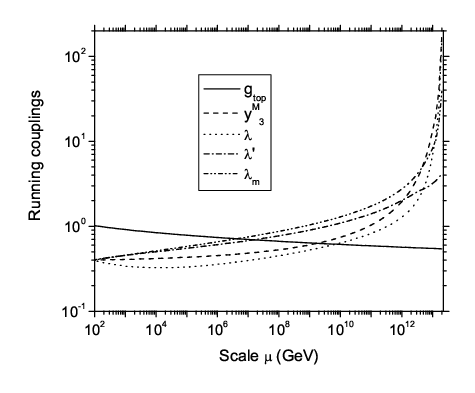
   For $g_{top}(100\,{\rm GeV})\approx 1$, and $y^{M}_{3}(100\,{\rm GeV})=\lambda(100\,{\rm GeV})=\lambda^{\prime}(100\,{\rm GeV})=\lambda_{m}(100\,{\rm GeV})=0.3$, (Set 1), we can see from Fig. 1 that their evolution from the EW scale ($100$ GeV) remains perturbative.

2. 2.

   On the other hand, for another set of parameters, $g_{top}(100\,{\rm GeV})\approx 1$, and $y^{M}_{3}(100\,{\rm GeV})=\lambda(100\,{\rm GeV})=\lambda^{\prime}(100\,{\rm GeV})=\lambda_{m}(100\,{\rm GeV})=0.4$ (Set 2), we find that the couplings blow up at an scale of O($10^{12}$), as it is shown in Fig. 2. Thus, just by going from $0.3$ to $0.4$, for the values of the parameters, we find a change of regime.

In what follows, we shall use Set 1 for the parameters of the Higgs potential. This scenario can be taken as an example where parameters have the maximal values allowed by the perturbativity criteria. Lower values are thus allowed too.

We are interested now in studying the new Higgs modes that appear in this model. We have evaluated the Higgs decays using the formulae presented in [21], with appropriate modifications to include the changes in couplings due to Higgs mixing. The decay width for the Higgs decay mode into a pair of majorons is given as follows:

In Ref. [16] we discussed the Higgs decays to neutrinos and their signatures in this model. The possible relation to Majoron Dark Matter has been considered in Ref. [22].

Here, using Eq. (13) one obtains the following decay widths ¹¹ 1 All SM decay widths will include an extra factor of $c_{\alpha}^{2}$:

In order to perform our numerical analysis, we shall take values allowed by the perturbative analysis (Set 1) for the parameters $\lambda_{m}$, $\lambda^{\prime}$, and some values for the vev $u$ and $\cos\alpha$. The mass of the Majoron $m_{\sigma}$ is given in terms of the parameter $u$ as follows:

For the light Higgs boson ($h$) we compute the BR’s of the different decay modes in the mass range $100\leq m_{h}\leq 200$ GeV, assuming that the heavier Higgs boson has a mass above 200 GeV, while the Majoron has a mass of the order tenths of MeV.

On the other hand, for the heavy Higgs boson ($H$) we consider the mass range $150\leq m_{H}\leq 500$, fixing the light Higgs boson mass with two values $m_{h}=114$ GeV and $m_{h}=160$ GeV.

We are also interested in determining whether the invisible Higgs decay could be observed at LHC. We shall use the results of Ref. [25], where a detailed study of detectability of an invisible Higgs was performed. These authors consider the production mechanisms $pp\rightarrow hZ^{0}$, for the signal, as well as $pp\rightarrow W^{+}W^{-}\rightarrow h$ and $pp\rightarrow h+jet$. Here, we shall use for illustration purposes, the associated production with $Z^{0}+h(\rightarrow inv.)$; a detailed set of cuts is proposed in order to determine the backgrounds [25]. Their analysis can be used to determine the minimum value of the ratio

We have explored in detail the Higgs phenomenology that results in a model where right-handed neutrinos have a mass scale of the order of the electroweak scale. In this model all scales arise from spontaneous symmetry breaking, and this is achieved with a Higgs sector that includes an extra Higgs singlet in addition to the standard model Higgs doublet. The scalar spectrum includes two neutral CP-even states ($h$ and $H$ with $m_{h}<m_{H}$) and a neutral CP-odd state ($\sigma$) that can be identified as a pseudo-Majoron.

The parameters that appear in the Higgs potential are essentially unconstrained by any phenomenology argument, therefore we have to resorted to some theoretical argument. Here we have relied on the perturbativity criteria, namely we have required that any choice of Higgs parameters at low-energies, which determine the Higgs spectrum and couplings, must remain below $4\pi$ when evolve from $m_{Z}$ up to a high-energy scale (such as $M_{GUT}$ or $M_{Planck}$).

Thus, we have explored the values of parameters $\lambda$, $\lambda^{\prime}$, $\lambda_{m}$, which satisfy the perturbative constraint $g_{i}(M_{GUT})$, $\lambda_{i}(M_{GUT})$ $<4\pi$, and we have identified some safe scenarios that are studied in this paper.

We have concluded that Set 1 ($g_{top}(100\,{\rm GeV})\approx 1$, and $y^{M}_{3}(100\,{\rm GeV})=\lambda(100\,{\rm GeV})=\lambda^{\prime}(100\,{\rm GeV})=\lambda_{m}(100\,{\rm GeV})=0.3$) can be taken as a scenario for the parameters of the Higgs potential having the maximal values allowed by the perturbative analysis.

The relevant Higgs BR and cross-sections are discussed, with special emphasis on the detection of the invisible Higgs signal at the LHC. We conclude that it could be possible to detect evidence of the existence of a pseudo-Majoron $\sigma$ through an invisible Higgs signal at the LHC for some values of parameters.

ACKNOWLEDGMENTS

The authors are grateful to Sistema Nacional de Investigadores and CONACyT (México) for financial support.

References

• [1] Q. R. Ahmad et al. [SNO Collaboration], Phys. Rev. Lett. 89, 011301 (2002) [arXiv:nucl-ex/0204008].
• [2] C. K. Jung, C. McGrew, T. Kajita and T. Mann, Ann. Rev. Nucl. Part. Sci. 51, 451 (2001).
• [3] K. Eguchi et al. [KamLAND Collaboration], Phys. Rev. Lett. 90, 021802 (2003) [arXiv:hep-ex/0212021].
• [4] M. H. Ahn et al. [K2K Collaboration], Phys. Rev. Lett. 90, 041801 (2003) [arXiv:hep-ex/0212007].
• [5] T. Schwetz, Phys. Scripta T127, 1 (2006) [arXiv:hep-ph/0606060].
• [6] M. Maltoni, T. Schwetz, M. A. Tortola and J. W. F. Valle, New J. Phys. 6, 122 (2004) [arXiv:hep-ph/0405172].
• [7] G. L. Fogli et al., Phys. Rev. D 75, 053001 (2007) [arXiv:hep-ph/0608060].
• [8] S. L. Glashow, Nucl. Phys. 22, 579 (1961); S. Weinberg, Phys. Rev. Lett. 19, 1264 (1967); A. Salam, Proc. 8th NOBEL Symposium, ed. N. Svartholm (Almqvist and Wiksell, Stockholm, 1968), p. 367.
• [9] Y. Fukuda et al. [Super-Kamiokande Collaboration], Phys. Rev. Lett. 81, 1158 (1998) [Erratum-ibid. 81, 4279 (1998)] [arXiv:hep-ex/9805021].
• [10] D. G. Michael et al. [MINOS Collaboration], Phys. Rev. Lett. 97, 191801 (2006) [arXiv:hep-ex/0607088]; S. Abe et al. [KamLAND Collaboration], Phys. Rev. Lett. 100, 221803 (2008) [arXiv:0801.4589 [hep-ex]].
• [11] For a review see: J. W. F. Valle, J. Phys. Conf. Ser. 53, 473 (2006) [arXiv:hep-ph/0608101].
• [12] A. Zee, Phys. Lett. B 93, 389 (1980) [Erratum-ibid. B 95, 461 (1980)].
• [13] P. Minkowski, Phys. Lett. B 67, 421 (1977).
• [14] M. Gell-Mann, P. Ramond and R. Slansky, Proceedings of the Supergravity Stony Brook Workshop, New York 1979, eds. P. Van Nieuwenhuizen and D. Freedman; T. Yanagida, Proceedings of the Workshop on Unified Theories and Baryon Number in the Universe, Tsukuba, Japan 1979, eds. A. Sawada and A. Sugamoto; R. N. Mohapatra and G. Senjanovic, Phys. Rev. Lett. 44, 912 (1980).
• [15] J. Schechter and J. W. F. Valle, Phys. Rev. D 22, 2227 (1980).
• [16] A. Aranda, O. Blanno and J. Lorenzo Diaz-Cruz, Phys. Lett. B 660, 62 (2008) [arXiv:0707.3662 [hep-ph]].
• [17] P. Q. Hung, Phys. Lett. B 649, 275 (2007) [arXiv:hep-ph/0612004].
• [18] M. L. Graesser, arXiv:0705.2190 [hep-ph].
• [19] A. de Gouvea, arXiv:0706.1732 [hep-ph].
• [20] E. Accomando et al. [CLIC Physics Working Group], arXiv:hep-ph/0412251.
• [21] J. Gunion, H. Haber, G. Kane and S. Dawson, The Higgs Hunter’s Guide, Addison-Wesley Publishig Company, Reading, MA, 1990.
• [22] A. Aranda and F. J. de Anda, Phys. Lett. B 683, 183 (2010) [arXiv:0909.2667 [hep-ph]].
• [23] L. Basso, S. Moretti and G. M. Pruna, arXiv:1004.3039 [hep-ph].
• [24] L. Basso, A minimal extension of the Standard Model with B-L gauge symmetry, (Master Thesis, Universitá degli Studi di Padova, 2007), at http://www.hep.phys.soton.ac.uk/∼\siml.basso/B-L Master Thesis.pdf.
• [25] H. Davoudiasl, T. Han and H. E. Logan, Phys. Rev. D 71, 115007 (2005) [arXiv:hep-ph/0412269].
Refer to caption
Figure 3: Braching ratios for the decay h→X​Xh\rightarrow XX with mσ=13​MeVm_{\sigma}=13\,{\rm MeV}, λ′=λm=0.1\lambda^{\prime}=\lambda_{m}=0.1 and three different values for cos⁡α\cos\alpha: (a) cos⁡α=0.1\cos\alpha=0.1, (b) cos⁡α=0.5\cos\alpha=0.5 and (c) cos⁡α≈1\cos\alpha\approx 1.
Figure 4: Braching ratios for the decay h→X​Xh\rightarrow XX with mσ=65​MeVm_{\sigma}=65\,{\rm MeV}, λ′=λm=0.1\lambda^{\prime}=\lambda_{m}=0.1 and three different values for cos⁡α\cos\alpha: (a) cos⁡α=0.1\cos\alpha=0.1, (b) cos⁡α=0.5\cos\alpha=0.5 and (c) cos⁡α≈1\cos\alpha\approx 1.
Figure 5: Braching ratios for the decay h→X​Xh\rightarrow XX with mσ=13​MeVm_{\sigma}=13\,{\rm MeV}, λ′=λm=0.3\lambda^{\prime}=\lambda_{m}=0.3 and three different values for cos⁡α\cos\alpha: (a) cos⁡α=0.1\cos\alpha=0.1, (b) cos⁡α=0.5\cos\alpha=0.5 and (c) cos⁡α≈1\cos\alpha\approx 1.
Figure 6: Braching ratios for the decay h→X​Xh\rightarrow XX with mσ=65​MeVm_{\sigma}=65\,{\rm MeV}, λ′=λm=0.3\lambda^{\prime}=\lambda_{m}=0.3 and three different values for cos⁡α\cos\alpha: (a) cos⁡α=0.1\cos\alpha=0.1, (b) cos⁡α=0.5\cos\alpha=0.5 and (c) cos⁡α≈1\cos\alpha\approx 1.
Figure 7: Braching ratios for the decay H→X​XH\rightarrow XX with mσ=13​MeVm_{\sigma}=13\,{\rm MeV}, λ′=λm=0.1\lambda^{\prime}=\lambda_{m}=0.1 and three different values for cos⁡α\cos\alpha: (a) cos⁡α=0.1\cos\alpha=0.1, (b) cos⁡α=0.5\cos\alpha=0.5 and (c) cos⁡α≈1\cos\alpha\approx 1.
Figure 8: Braching ratios for the decay H→X​XH\rightarrow XX with mσ=65​MeVm_{\sigma}=65\,{\rm MeV}, λ′=λm=0.1\lambda^{\prime}=\lambda_{m}=0.1 and three different values for cos⁡α\cos\alpha: (a) cos⁡α=0.1\cos\alpha=0.1, (b) cos⁡α=0.5\cos\alpha=0.5 and (c) cos⁡α≈1\cos\alpha\approx 1.
Figure 9: Braching ratios for the decay H→X​XH\rightarrow XX with mσ=13​MeVm_{\sigma}=13\,{\rm MeV}, λ′=λm=0.3\lambda^{\prime}=\lambda_{m}=0.3 and three different values for cos⁡α\cos\alpha: (a) cos⁡α=0.1\cos\alpha=0.1, (b) cos⁡α=0.5\cos\alpha=0.5 and (c) cos⁡α≈1\cos\alpha\approx 1.
Figure 10: Braching ratios for the decay H→X​XH\rightarrow XX with mσ=65​MeVm_{\sigma}=65\,{\rm MeV}, λ′=λm=0.3\lambda^{\prime}=\lambda_{m}=0.3 and three different values for cos⁡α\cos\alpha: (a) cos⁡α=0.1\cos\alpha=0.1, (b) cos⁡α=0.5\cos\alpha=0.5 and (c) cos⁡α≈1\cos\alpha\approx 1.