Toward Regional Characterizations of the Oceanic Internal Wavefield
Abstract
Many major oceanographic internal wave observational programs of the last four decades are reanalyzed in order to characterize variability of the deep ocean internal wavefield. The observations are discussed in the context of the universal spectral model proposed by Garrett and Munk. The Garrett and Munk model is a good description of wintertime conditions at Site-D on the continental rise north of the Gulf Stream. Elsewhere and at other times, significant deviations in terms of amplitude, separability of the 2-D vertical wavenumber - frequency spectrum, and departure from the model’s functional form are reported.
Specifically, the Garrett and Munk model overestimates annual average frequency domain spectral levels both at Site-D and in general. The bias at Site-D is associated with the Garrett and Munk model being a fit to winter time data from Site-D and the presence of an annual cycle in high frequency energy in the western subtropical North Atlantic having a maximum in winter. The wave spectrum is generally non-separable, with near-inertial waves typically having greater bandwidth (occupying smaller vertical scales) than continuum frequency waves. Separability is a better approximation for more energetic states, such as wintertime conditions at Site-D. Subtle geographic differences from the high frequency and high vertical wavenumber power laws of the Garrett and Munk spectrum are apparent. Such deviations tend to co-vary: whiter frequency spectra are partnered with redder vertical wavenumber spectra.
We review a general theoretical framework of statistical radiative balance equations and interpret the observed variability in terms of the interplay between generation, propagation and nonlinearity. First: Nonlinearity is a fundamental organizing principle in this work. The observed power laws lie close to the Induced Diffusion stationary states of the resonant kinetic equation describing the lowest order nonlinear transfers. Second: Eddy variability and by implication wave-mean interactions are also an organizing principle. Observations from regions of low eddy variability tend to be outliers in terms of their parametric spectral representation; other data tend to cluster in two regions of parameter space. More tentatively, the seasonal cycle of high frequency energy is in phase with the near-inertial seasonal cycle in regions of significant eddy variability. In regions of low eddy variability, the seasonal cycle in high frequency energy lags that of near-inertial energy.
The Induced Diffusion stationary states are approximate analytic solutions to the resonant kinetic equation and the Garrett and Munk spectrum represents one such analytic solution. We present numerical solutions of the resonant kinetic equation, though, that are inconsistent with the Garrett and Munk model representing a stationary state, either alone or in combination with other physical mechanisms. We believe this to be the case for other regional characterizations as well. We argue that nonstationarity of the numerical solutions is related to local transfers in the horizontal wavenumber domain whereas the analytic Induced Diffusion solutions consider only nonlocal transfers in the vertical wavenumber domain. Consequences for understanding the pathways by which energy is transfered from sources to sinks are considered. Further progress likely requires self-consistent solutions to a broadened kinetic equation.
Polzin and Lvov \titlerunningheadRegional Characterizations \authoraddrK. L. Polzin MS#21, Woods Hole Oceanographic Institution, Woods Hole, MA 02543, USA. (kpolzin@whoi.edu) \authoraddrY. V. Lvov Department of Mathematical Sciences, Rensselaer Polytechnic Institute,Troy NY 12180, USA. (lvovy@rpi.edu)
1 Introduction
Internal waves are ubiquitous features of geophysical fluids, contain a significant fraction of the total variance and constitute an effective mechanism for transferring energy and momentum across large distances and across different scales. In particular, the drag associated with internal wave breaking needs to be included in order to obtain accurate simulations of the atmospheric Jet Stream (Fritts et al., 2003) and it has been argued that the ocean’s Meridional Overturning Circulation (Wunsch and Ferrari, 2004) is forced by the diffusion of mass (Ledwell et al., 2000) associated with internal wave breaking (Polzin et al., 1997) rather than by the convective production of cold, dense water at high latitudes. Both circulations represent fundamental pieces of the Earth’s climate system.
The oceanic internal wavefield is ”complex”. It spans a vast range of scales: in the time domain periods range from about one day for inertial waves to a few minutes for buoyancy frequency waves in the pycnocline. Horizontal wavelengths range from a few meters to hundreds of kilometers. The internal wave field’s complexity arises not just from its extended range of scales, but also from a multiplicity of possible sources at the surface (atmospheric forcing associated with wind stress and buoyancy fluxes) and bottom (tides and mean currents impinging upon nonuniform topography); the potential for scale transformations (reflection and scattering from topography) and dissipation at the bottom boundary; and interior transfers of energy and momentum through wave-mean flow interactions. A significant sink is wave breaking, which is believed to be product of nonlinearity resulting in downscale transfers of energy.
Despite, or perhaps because of, this complexity, a universal character is usually ascribed to the oceanic internal wave energy spectrum. In a classic work, Garrett and Munk (1972) demonstrated how observations from various sensor types could be synthesized into a combined wavenumber-frequency spectrum, now called the Garrett-and-Munk (GM) spectrum of internal waves. Consistent only with linear internal wave kinematics, the GM spectrum was developed as an empirical curve fit to available data. Deviations have been noted near boundaries (Wunsch and Webb, 1979; Polzin, 2004b) and at the equator (Eriksen, 1985a). However, our notion of what constitutes the background wavefield has remained static since the last significant model revision provided by Cairns and Williams (1976).
The authors’ sentiments are captured by the first paragraph of Briscoe (1975a)’s Survey section: “The single paper motivating the most comments, experiments, and disquiet in a lot of readers was Garrett and Munk (1972), now called familiarly GM72. (The updated version is Garrett and Munk (1975), called GM75.) The paper is a virtuoso orchestration of synthesis, approximation, boldness, normalization, and implication. Starting from the observation that the wavenumber-frequency () spectrum of a multimodal dispersive system is not uniquely determined by pure wavenumber and pure frequency spectra, the paper goes onto construct from linear dynamics and WKBJ methods an spectrum that is astonishingly consistent with many kinds of data from all kinds of instruments. Wunsch (1975) iconoclastically discusses the pitfalls of such an approach and correctly emphasizes the fact that the dynamically important trait is the inconsistency of various data sets with some base state model.” With immense inspiration provided by Garrett and Munk, we take up, after 35 years, the difficult task posed by Wunsch. We document variability of the oceanic internal wavefield and then review the field to assess the dynamical underpinnings of that variability. While heavily referenced, this work does not attempt to be a literature review.
In previous work (Lvov et al., 2004) we noted that deviations of frequency/vertical wavenumber power laws from the universal model tend to co-vary: whiter frequency spectra are partnered with redder vertical wavenumber spectra. Here we provide a more systematic study of such deviations. We define spatial and temporal patterns of spectral parameters (amplitude, power laws, bandwidth and separability) in a review of many observational programs of the last four decades. Having documented variability in the background wavefield, we interpret the spatial patterns in terms of generation, nonlinearity, wave-mean interactions and dissipation.
Nonlinearity plays a key role. In a companion manuscript (Lvov et al., 2010) we discuss the application of wave turbulence formalisms to this problem and rigorously demonstrate the validity of conventional wisdom regarding a truncated analytic approximation to nonlinear spectral transfers described in McComas and Müller (1981a); McComas and Müller (1981b). The observed power law combinations in frequency and vertical wavenumber documented here are largely consistent with the stationary states associated with the truncated analytic approximations. While this appears to be a stunning affirmation of this approximation to the wave turbulence transfer integral, it comes with caveats, disclaimers and possible contradictions. First, the theory is not formally valid at high wavenumber for realistic wave amplitudes. Second, the identification of GM76 being a stationary state is only true after integration over the frequency domain and invocation of dissipation. Finally, numerical evaluations of the nonlinear transfers are inconsistent with the high frequency, high vertical wavenumber domain of GM76 being a stationary state. This tension also applies to other stationary states identified by the truncated analytic theory having power law combinations associated with energy transfers from larger to smaller vertical scales and from higher to lower frequencies. Such stationary states require an energy source at high frequencies. But our review of the remaining generation and spectral transport mechanisms does not yet reveal what this mechanism might be.
The article is organized as follows. In Section 2 we summarize the development of the GM model through its various incarnations. We then review and re-analyze data obtained by major internal wave observational programs of the last four decades in Section 3. These data clearly demonstrate that deviations from the GM spectrum are not random, but rather form a distinct pattern which we summarize in Section 4. We discuss the theoretical framework which may be used to interpret these observations in Section 5 and conclude in Section 6. An appendix contains additional useful information relating to the interpretation of oceanographic data.
2 Background
2.1 Kinematic Structure
2.1.1 Dispersion Relation
Internal waves arise through the restoring force of gravity in a stably stratified fluid. In a rotating system they comprise a ’fast’ mode of oscillation with frequencies between inertial and buoyancy frequencies. In terms of an Eulerian description with velocity vector , the linearized equations of motions are
in which kinematic pressure and buoyancy are perturbations from a hydrostatically balanced equilibrium state, , is gravity and the fluid is assumed to be incompressible (). We use as a position vector. An over-bar indicates a mean on time scales much longer than a wave period. The constant is the mean density and arises from assuming density to be constant in computing momentum changes associated with accelerations, but taking density changes into account when they give rise to buoyancy forces (the Boussinesq approximation). The buoyancy gradient relates to oscillations of frequency corresponding to periods of minutes in the upper ocean to hours in the abyss. This work is concerned almost exclusively with horizontal scales small enough that the Earth’s rate of rotation about the local vertical, , can be considered as constant (the f-plane approximation). The rate of rotation of the Earth about its axis is . The Coriolis frequency thus corresponds to periods of 1/2 day at the poles to several days in the tropics and vanishes at the equator. The foundation for interpreting observations lies in linear polarization relations (Section 2.1.2) obtained from these equations of motion.
The equations of motion can be manipulated to obtain a wave equation in vertical velocity (e.g., Gill (1982)):
| (1) |
for arbitrary stratification profile . Assuming the background stratification is constant, plane wave solutions with three dimensional wavevector having vertical component and horizontal magnitude return
| (2) |
which can be rewritten as
Many of the important properties of internal waves are immediately available:
- •
Incompressibility and a plane wave solution imply particle velocities are normal to the wavevector, .
- •
Freely propagating waves, for which is real, require .
- •
Wave frequency solely determines the angle of the wavevector relative to the vertical and, since , the ratio of horizontal to vertical velocity.
- •
The group velocity if ) has the ’odd’ property that crests and troughs (i.e., lines of constant phase) propagate in the same direction as a wave packet (group) in the horizontal but the signs of phase and group velocity differ in the vertical coordinate. Upward phase propagation implies downward energy propagation.
2.1.2 Polarization Relations
A suite of diagnostic relations can be obtained by assuming constant stratification rate, plane wave solutions in which all variables are proportional to and expressing the dependent variables in terms of wave amplitude :
| (3) | |||||
| (4) | |||||
| (5) | |||||
| (6) | |||||
| (7) |
The prefactor in these polarization relations is such that the wave amplitude is normalized to represent the total energy:
| (8) |
The total energy is the sum of horizontal kinetic , vertical kinetic and potential energy in which represents the vertical displacement.
Two important diagnostics utilized here are: First, assuming constant stratification, the ratio of horizontal kinetic to potential energy for a single internal wave is:
| (9) |
Second, the horizontal velocity trace for high frequency internal waves is rectilinearly polarized. Rotation alters this so that the velocity trace at inertial frequency inscribes a circle with time. With depth, the near inertial velocity vector traces out an elliptical helix in which the ratio of velocity variance in the clockwise () and counter-clockwise () rotating components is given by:
| (10) |
with the sign convention that positive frequency implies upward phase propagation (and hence downward energy propagation) in the northern hemisphere.
2.1.3 Weak Spatial Inhomogeneities
If the stratification profile varies much more slowly than the wave phase, a WKB approximation for vertically propagating waves provides the approximate solution to (1):
| (11) |
and so the effects of a variable buoyancy profile can be accounted for by stretching the depth coordinate by . This amounts to scaling the vertical wavenumber by , in which is a reference stratification. The value 3 cph is often used. The buoyancy scaling of other dependent variables follows from the polarization relations (3)-(7). The use of the WKB approximation requires . If this relation is not satisfied, solutions can be found by treating (1) as an eigenvalue problem with appropriate boundary conditions. If but the wave-phase is not slowly varying, the boundary conditions are that at the top () and bottom (), which then implies the horizontal velocities are proportional to:
| (12) |
for integer values of n.
Similarly, one can investigate interactions of the internal wavefield with a mean velocity field by assuming the internal wavefield has small amplitude and small spatial scales relative to a time independent geostrophically balanced flow, Section 5.2. This problem is amenable to WKB and ray-tracing techniques. In this slowly varying limit, the linear polarization relations reported here are modified by replacing the Eulerian frequency with the intrinsic frequency .
2.1.4 Slow Oscillations
Internal waves are to be distinguished from a ’slow’ mode consisting of, at lowest order, the steady geostrophic balance.
Higher order contributions are time dependence, nonlinearity and the effects of a variable rate of planetary rotation (). Substitution of a plane wave solution into the geostrophic balance returns primarily the information that small aspect ratio fluctuations () have ratios of less than one.
There are two main paradigms for considering these slow motions vis-a-vis the fast internal wavefield. The first, already alluded to, is the limit that geostrophic velocities are larger and have significantly larger spatial scales. The second paradigm comes about as the two share similar spatial scales. In this instance the slow motions have typically smaller amplitudes and hence appear as a ’contamination’ to the wavefield. Beyond the issue of aspect ratio, the consistency relations for this non-propagating mode have little utility and this ’contamination field’ has the character of uncorrelated noise, which is the content of several diagnostic studies (D’Asaro and Morehead, 1991; Kunze and Sanford, 1993). The characterization of this slow mode as ’noise’ should not surprise. The dynamics in this limit are those of stratified rotating turbulence in which motions at different isopycnals are uncoupled at scales larger than those over which shear instabilities can develop (Riley and Lelong, 2000).
While diagnostic models of the slow mode usually assume an incoherent field (Müller et al., 1978), the interaction of the internal wavefield with quasi-permanent density finestructure can be exploited by assuming the wavefield buoyancy scales on the density finestructure (Polzin et al., 2003). This buoyancy scaling results in a correlation between internal wave shear and quasi-permanent density gradients when such a correlation is inconsistent with fields composed of either pure waves or pure finestructure. This enables an estimate of the quasi-permanent spectrum, Polzin et al. (2003) and Section 3.3.4.
One finestructure consistency relation has great importance. The plane wave solutions of internal waves have no Ertel potential vorticity signature, whereas the non-waves have non-zero Ertel potential vorticity (Müller et al., 1986). The distinction is important for issues of isopycnal dispersion (Polzin and Ferrari, 2004) and for dynamics (Müller, 1995).
Reliance upon the plane wave solutions, however, has its limitations. While internal waves and slow modes can be distinguished in terms of Ertel potential vorticity content, this distinction disappears when one considers a slowly varying wavepacket with spatial structure in both horizontal directions, i.e., solutions of the form
See Bühler and McIntyre (2005) and Polzin (2008a) for further details.
2.2 Parametric Spectral Representations
Much of the original Garrett and Munk (1972) paper is a demonstration of how observations from various sensor types could be synthesized into a combined wavenumber-frequency spectrum consistent with linear internal wave kinematics. The toolbox contains:
- •
- •
diagnostic relations (Section 2.1.2) to test consistency with linear wave kinematics, and
- •
the choice of a vertical spectral rather than modal representation implies the invocation of an ‘equivalent continuum’ in which the waves are assumed to be vertically propagating. Boundary conditions and turning points are neglected. See Garrett and Munk (1972) for a discussion of modal properties.
Assuming that the buoyancy profile varies much more slowly than the wave phase implies the total energy , obtained as an integral of the energy density over the spectral domain,
| (13) |
varies as
| (14) |
i.e., is an adiabatic invariant. The energy spectrum is denoted as with following arguments [e.g., ]. The variable without following arguments represents total energy.) The factors and represent reference values for the total energy of the internal wavefield and stratification.
Garrett and Munk proposed that the spectral energy density can be represented as a separable function, i.e., the product of a function of vertical wavenumber only and function of wave frequency only:
| (15) |
where is a fixed reference number. This reference wavenumber is conveniently expressed as
| (16) |
in which the variable represents the mode number of an ocean with an exponential buoyancy frequency profile having a scale height of [ = 1300 m in the GM model]. Separability in vertical wavenumber and frequency was invoked as the simplest representation not inconsistent with available data. The spectral amplitude was regarded as being independent of spatial coordinate apart from the dictates of buoyancy scaling. Use of non-separable and anisotropic parametric spectral representations can be found in Müller et al. (1978).
Functions and should be normalized to unity, so that the integrals
and
are dimensionless and in practice the limits of integration ( represents vertical mode-1, a high wavenumber cutoff of approximately 0.1 cpm) are approximated for analytic convenience. The high wavenumber cutoff, defined by
| (17) |
represents an observed transition to steeper spectral slopes and likely signifies a dynamical transition to a more strongly nonlinear, yet not turbulent, regime.
The GM model evolved over time, resulting in three major versions, denoted GM72, GM75 and GM76:
| (20) | |||||
and
| (22) |
The gamma function () appears in the normalization for the vertical spectrum. All versions of GM utilize and , so that
Both functions and behave as power-laws at high wavenumber and frequency; has an integrable singularity at the inertial frequency (which constrains ), and has a plateau for small value of its argument. As explained below these features were found to be representative of the oceanic internal wave field.
The total energy in the model,
| (23) |
is based upon fits to observed high frequency spectra rather than estimates of total observed internal wave band energy.
2.3 The GM model’s three incarnations
The GM model evolved over time as more and better data became available. This section documents reasons behind the choice of specific parameters.
2.3.1 Frequency Domain
While Garrett and Munk (1972) noted variability in the tidal peak, the tides are not part of the GM model. The specific shape of the inertial peak was simply chosen out of analytic convenience. Variability in the frequency domain power law was apparent even then, with a noted alternative being (Webster, 1969). With many possible ’noise’ sources such as mooring motion and finestructure contamination serving to whiten the frequency spectrum, the judicious choice for a model of the background spectrum is a redder (Section 3.3.1). This choice remains stable throughout the various model versions.
2.3.2 Vertical Wavenumber Domain
The spatial domain information available in the late-1960’s was limited to stationary current meters and horizontally towed thermistor chains. The direct information available from current meters was through spatial lag coherences11 1 Estimates of vertical bandwith can be obtained by assuming a parametric spectral representation and fitting lagged coherence estimates to the inverse Fourier transform of the spectrum, (Garrett and Munk, 1972; Cairns, 1975; Müller et al., 1978). This technique can be found in many textbooks as the Wiener-Khinchine relation.. The towed data return both a direct estimate of the horizontal spectrum and vertical lag coherence information. These data supported only a crude representation of the vertical wavenumber spectrum as a top-hat model with about 20 equivalent modes excited ( in GM72).
The quality of the information improved dramatically in the early 1970’s with the introduction of near-continuous vertically profiling instrumentation such as the Neil Brown CTD (Brown, 1974) and Tom Sanford’s electric field sensing device (Sanford, 1975). The choice of which data to rely upon, though, is quite subjective and the perception is that finestructure contamination of the density field is more problematic than contamination of the velocity field, e.g., Polzin et al. (2003). See Section 3.3.2 for a discussion of the Sanford (1975) data set. Extant temperature gradient spectra tended to be white at an intermediate range of vertical wavenumbers (roughly 0.01 0.2 cpm) and roll off thereafter. GM75, however, relied upon even higher wavenumber CTD data from Millard (1972), ignored possible inconsistencies with CTD data in Hayes (1975), and heavily weighted the velocity profile data in Sanford (1975) to argue for a high wavenumber slope . Estimates of isotherm fluctuations from a vertically profiling float (Cairns, 1975) suggested a much lower bandwidth () than in the GM72 model.
GM75 was soon replaced by a more refined model. Further analysis of float data by Cairns and Williams (1976) suggested revision of the high wavenumber power law to and a change to the functional form . The rationale given for choosing such a functional form is simply its analytic convenience: has a simple cosine transform, see also Desaubies (1976). Munk (1981) follows suit. This revision is labeled GM76. The distinction between and is in the rapidity of the roll-off from the low-wavenumber plateau region to the high-wavenumber asymptote. GM76 has a more rapid transition than GM75 for equivalent power laws.
3 Observations of Internal Wave Spectra
3.1 Observational framework/preliminary notes
Observations of the oceanic internal wave field are analyzed in this section in order to define the extent to which the deep ocean internal wavefield is indeed universal. We follow the lead of GM by characterizing observed spectra with the parametric power law representations (2.2) and (22) and also allow for variable spectral levels with the focus upon identifying spatial/temporal variability of the spectral parameters.
Variability in the frequency domain is quantified by fitting
| (24) |
to the high frequency portion of the observed spectra. ’High’ frequency refers to periods less than 10 hours, thereby eliminating the inertial peak and semi-diurnal tides from consideration. The amplitude is reported as a fraction of the energy associated with the GM spectrum:
| (25) |
An additional reported statistic is the total internal wave band energy in the observed spectrum. Internal wave band energy is estimated by integrating the observed frequency spectra over frequencies greater than approximately 0.7, thereby including broadening of the inertial cusp.
Variability in the vertical wavenumber domain is quantified by fitting variants of (2.2) to the observed spectra. The resulting statistics are less satisfactory than those in the frequency domain as low wavenumbers are not well resolved in most instances.
3.2 Some words of caution
Power laws are an attractive and simple way to describe complex systems in general and internal waves in particular. Some details of the observed spectra may defy this simple approach. Our view is to treat the parametric representation as a general tendency to help summarize and interpret otherwise complicated data. With that caveat, there is no shortage of reasons for the observed variability: nonlinearity, instrumentation, the buoyancy profile, low frequency flows, tides, bathymetry, horizontal inhomogeneity, vertical asymmetry and contamination by either quasi-permanent finestructure or self advection (Doppler shifting) within the internal wavefield:
- •
It matters how you look at the ocean. Instrument response and processing methods may affect the interpretation. An appendix contains remarks to aid the reader in negotiating this maze.
- •
All that wiggles is not necessarily an internal wave. Internal waves typically dominate the small scale variability and geostrophically balanced motions dominate the largest scales. But quasi-permanent finestructure has been identified as making an increasing contribution to the total spectrum at high wavenumber (e.g., Müller et al. (1978); Polzin et al. (2003), Section 2.1.4).
- •
In many cases, the quoted spectral power laws are derived from one-dimensional (vertical wavenumber and frequency) spectra. Thus there is an implicit assumption that the spectra are separable, (15). Since both 1-d spectra are red, frequency spectra are typically dominated by low vertical wavenumber motions and vertical wavenumber spectra are dominated by low frequencies. The one-dimensional power laws are not identical to the 2-d power laws if the spectra are non-separable.
- •
The sampling strategy matters. Vertical wavenumber-frequency domain information are seldom obtained from a single instrument, nor are the measurements taken instantaneously. Vertical profile data obtained as a spatial survey can be used to define a spatial mean and residuals, and the internal wave contribution identified as the residual field. However, this will alias some low-frequency variability into the residual fields. Vertical profile data obtained as a time series can effectively separate the internal wave variability from lower frequency motions. But the resulting residuals may not be representative of the background wavefield: that background may be temporarily distorted, for example, by wave-mean interactions.
- •
Anisotropic propagation in a region of variable stratification or into/away from a critical layer can imply significant transport of energy in the vertical wavenumber domain and thereby create apparent structure unrelated to nonlinearity.
- •
The results presented here are primarily from analyses in depth or pressure coordinates, rather than in an isopycnal coordinate system. High frequency Eulerian spectra are prone to Doppler shift contamination at high vertical wavenumber. Use of an isopycnal coordinate system limits the Doppler shift contamination (Sherman and Pinkel, 1991).
Despite these limitations, we believe that the patterns of spatial and temporal variability discussed below reflect physical reality and are not an artifact of processing or interpretation.
3.3 A Regional Catalog
![[Uncaptioned image]](1007.2113v2/Atlantic_GC.png)
|
|
|---|---|
![[Uncaptioned image]](1007.2113v2/Pacific_GC.png)
|
|
Variability of the oceanic internal wave spectrum will likely exist on multiple temporal and spatial scales, e.g., those scales associated with individual wave packets and isolated forcing events. In the present study we assume that differences in the background spectrum are a product of regional differences in forcing and boundary conditions averaged over the characteristic time scale to dissipate the energy resident in the internal wavefield (about 50 days) and averaged over the characteristic spatial scale that internal waves can propagate in that time span. The forcing mechanisms and propagation scales are, in general, not regionally well defined.
Thus multiple data sets from Site-D (north of the Gulf Stream), the Sargasso Sea and the California Current System are grouped together (Fig. 1). In terms of low frequency variability, Site-D exhibits the largest eddy energy, e.g., Wunsch (1997). Eddy energies in the Sargasso Sea and California Current System exhibit spatial trends but are comparable to each other. Short narratives are used to document regional characterizations of eddy amplitudes, tides and bottom topography.
3.3.1 Site D - and .

Site-D was fourth of a series of stations on a section from Woods Hole to Bermuda. Historically, the technology for long term current meter deployments was developed in Woods Hole, and Site-D served as the test bed for much of that instrumentation. Much of the data in the original Garrett and Munk paper (GM72) came from Site-D, if for no other reason than not much else was available. Site-D is characterized by a relatively small amplitude tide and large low-frequency (predominantly Topographic Rossby Wave) activity, e.g., Hogg (1981). Site-D is situated under the Eastern Seaboard storm track, resulting in an enhanced potential for the resonant coupling between windstress and mixed layer at near-inertial frequencies (D’Asaro, 1985). Site-D may be relatively unique because of its geographic location.
It is apparent that, although many data were under consideration in Garrett and Munk (1972), the GM72 model is a curve fit to the original Site-D data presented in Foffonoff (1969) in both amplitude and power law (Fig. 2)22 2 Departures from a simple power law behavior are apparent in the thermocline data at high frequencies and spectra from the deeper current meters do not roll-off at frequencies exceeding the local . Data from the very stable trimoored IWEX mooring roll-off nicely (see below) and thus Briscoe (1975b) suggests the super-buoyancy extension is an artifact of mooring motion. On the other hand, this does not mean that the departures from a simple power law behavior apparent in the upper current meters is an artifact of mooring motion. See Appendix B.1 for further details.. The GM72 model is a good characterization of the spectral shape at Site-D throughout the decades (Fig. 3). However, variability is apparent in spectral amplitude.

The original (1967) Site-D data are characterized by larger spectral levels than the other, longer term, estimates. Briscoe and Weller (1984) document an annual cycle in high frequency internal wave energy using data from the Lotus region south of the Gulf Stream, with maximum values in winter. This annual cycle is also apparent in the Primer data from Site-D (Fig. 4). A seasonal cycle in near-inertial energy for this location is discussed in detail in Silverthorne and Toole (2009).
With the GM spectrum being a curve fit to the early (1967) data, and with those data being obtained in February-March, the GM model is essentially a description of the winter time spectrum at Site-D. The summer time spectrum has lower amplitude with little change in spectral slope at high frequency (Fig. 5). We anticipate results presented below by stating here that annual average spectral levels at Site-D tend to be larger than other places and thus the Garrett and Munk model is a poor description of the background internal wavefield in much of the World Ocean.


Despite the vertical spectrum being defined using data obtained elsewhere, recent vertical profile data data from Site-D are remarkably consistent with the GM76 model [] (Fig. 6). Wintertime conditions exhibit both enhanced spectral levels (amplitude factors of 2.75 vs 1.75) and relatively more variance at low modes ( vs ) than summertime data. Winter time conditions also exhibit larger ratios of kinetic-to-potential energy at high wavenumber, implying an increased input of near-inertial energy during winter time and relaxation to higher frequencies.


3.3.2 The Sargasso Sea
A large number of experiments have been located in the Sargasso Sea over the Hatteras Abyssal Plain. On the southern side of the Gulf Stream, this region exhibits an energetic eddy field having significant north-south gradients. Eddy energy levels are typically less than noted at Site-D. A tidal () peak is apparent in the temperature and velocity spectra. Müller et al. (1978) find that fluctuations at this frequency have larger characteristic vertical scales than the internal wave continuum, and there is evidence of similar features at the first several harmonics. From current meter data at 28∘N, 70∘W Noble (1975) and Hendry (1977) estimate net fluxes at to be to the southeast and infer the source to be the Blake Escarpment, near the western boundary. Alford and Zhao (2007), on the other hand, document net semidiurnal fluxes to the north-northwest (at 31∘N, 69W ) and southwest (at 34∘N, 70∘W ).
The bottom near mid-basin is well sedimented and smooth at 28∘N, 70∘W, the locus of the Mid-Ocean Dynamics Experiment and the Internal Wave Experiment. Rougher topography is noted to the east33 3 One also finds mud waves. Mud waves are sedimentary features of 1-10 km horizontal wavelength having amplitudes of 10’s to 100’s of meters. These horizontal scales are appropriate for the generation of freely propagating internal lee waves (with Eulerian frequency ) if the intrinsic frequency lies between the Coriolis and buoyancy frequencies: . Significant coupling between the ’mean’ and internal wavefield is anticipated at mean flow rates of 0.1-0.2 m s-1. Sediment transport is an issue at such flow rates and the possibility exists that the lee wave velocity perturbations affect the deposition/erosion process so as to reinforce the mud-waves (Blumsack, 1993). But this gets us off the topic of the background internal wavefield.. The PolyMode Local Dynamics Experiment current meter array (at 31∘N, 69W ) is likely situated above relatively rough terrain. Bathymetry is relatively smooth at 34∘N, 70∘W, the locus of the Long Term Upper Ocean Study.
The buoyancy frequency profile has a relative minimum in associated with the 18∘ water thermostad at
about 300 m water depth. The main thermocline exhibits nearly
constant stratification between 500-1000 m.
MODE
Conducted during March-July of 1973, the Mid-Ocean Dynamics Experiment (MODE) was one of the first concentrated studies of mesoscale ocean variability. The experiment featured arrays of moored current meters, neutrally buoyant floats, standard hydrographic station techniques and the use of novel vertically profiling instrumentation. An extensive array of current meter moorings was deployed in a 300 km radius centered about ( N, W). Data return from the current meters was limited (Mode Atlas, 1977).
While designed primarily to investigate low frequency motions, the experiment returned a great deal of information about internal waves. Vertical profiles of horizontal velocity obtained during May and June with a free-falling instrument using a electric field sensing technique Sanford (1975) provided, for the first time, direct estimates of the high vertical wavenumber structure of the ocean internal wavefield. These data are dominated by near-inertial frequencies, and a rotary decomposition in the vertical wavenumber domain Leaman and Sanford (1975) reveals a large excess of clockwise () phase rotation with depth. Clockwise phase rotation with depth is a signature of downward energy propagation for near-inertial waves.
Despite the evidence of excess downward energy propagation that was interpreted in terms of atmospheric generation (Leaman, 1976), these data were assumed to be representative of the background internal wavefield. A subset obtained as a time series of days provided the basis for a revision to the isotropic Garrett and Munk spectral model, GM75, with high wavenumber asymptote of .
The MODE profile data were included in our original study (Lvov et al., 2004)
reporting the covariability of frequency-wavenumber power laws.
Further investigation suggests the characterization of these data as
representing the background wavefield is problematic. Several
coherent wavepackets dominate the high wavenumber energy content and
these packets can be interpreted as being strained by the mesoscale
eddy field and propagating into a critical layer (Polzin, 2008a). Thus
wave-mean interactions acting in conjunction with the downward
propagating waves may be responsible for creating structure in the
vertical wavenumber domain uncharacteristic of the background
spectrum.
IWEX - and
The Internal Wave Experiment (IWEX) represents an early attempt to estimate a vector wavenumber-frequency spectrum with a minimum of assumptions. Current and temperature data were obtained with 17 Vector Averaging Current Meters (VACMs) and 3 Geodyne 850 current meters from a taut, three-dimensional, trimoored array.
Müller et al. (1978) assumed the spectrum could be factorized as:
with denoting the sign of vertical energy propagation, the normalized horizontal wavenumber () distribution and a normalized azimuthal () distribution. Their horizontal wavenumber distribution was assumed to have a parametric representation of:
for and otherwise. The parameters are horizontal wavenumber scale , low wavenumber cut-off , shape factor , and high wavenumber slope . An inverse analysis of the spatial lag cross spectra (the lag-coherence is proportional to the Fourier transform of the energy spectrum) was performed to estimate the various parameters in their proposed spectrum. In particular, Müller et al. (1978) find that the horizontal wavenumber energy spectrum depends upon wavenumber as , independent of frequency. For continuum () frequencies the horizontal and vertical wavenumber power laws are identical. Thus . The observed frequency spectra of both velocity and temperature are characterized by the power law , Briscoe (1975b) (Fig. 7).
The Müller et al. (1978) analysis includes an estimate of finestructure contamination. That is, their horizontal wavenumber spectrum includes only contributions which are consistent with linear internal waves. An increasing contamination with increasing frequency (decreasing horizontal scale) is apparent. As they make no distinction between permanent finestructure contamination and Doppler shifted internal waves, much of their finestructure contamination could be internal waves [e.g., Sherman and Pinkel (1991); Polzin et al. (2003)]. Thus the horizontal wavenumber domain power law estimate may be biased too steep.
Several features of the IWEX data set reoccur in many of the other data sets analyzed here. The first is that estimates of amplitude based upon fits to the high frequency part of the spectrum tend to be significantly lower than the GM model whereas estimates of total energy tend to be more nearly equal to the total energy in the GM model. The inference is that the inertial cusp of the GM model is not sufficiently strong to describe the oceanic peak. While this has been noted before (e.g., Fu (1981)), the IWEX analysis indicates the excess near-inertial energy has smaller characteristic vertical scales: At super-tidal frequencies the peak wavenumber corresponds to the first vertical mode. At near-inertial frequencies corresponds to the third vertical mode, indicating significantly reduced near-inertial energy in the first two modes. This pattern is consistent with the vertical profile data presented here which depict ratios of to at 100 (1000) m. vertical wavelengths that are significantly larger (smaller) than in the GM model, for which .
Müller et al. (1978) avoid interpreting the IWEX spectrum in the context of how
it might relate to the background oceanic spectrum. This is not
surprising given the short duration of the data set and the relative
lack of quality data sets at that time. Here, however, we promote the
IWEX spectrum as a more realistic representation of the Sargasso Sea
background spectrum than the GM model.

LOTUS - –
One goal of the Long-Term Upper-Ocean Study (LOTUS) was to document variability in the internal wavefield over several seasons in order to investigate its association with a variety of forcing mechanisms and environmental conditions. Meteorological data were obtained with a surface mooring and buoy. Only data from subsurface moorings are described here. The region is notable for extreme air-sea buoyancy exchange resulting in the production of Eighteen Degree Water, e.g., Kwon and Riser (2004)
Briscoe and Weller (1984) document an annual cycle of high frequency internal wave energy at 200-500 m depths from the first year’s data. The energy was noted to vary from a half or a third to 2 or three times the mean at each depth. That signal is repeated in the second year’s data (Fig 8). Apart from the seasonal cycle, internal wave energy varies on time scales of several weeks. The relation between this short time scale variability and low frequency (sub-inertial) shear has been noted since MODE (see Ruddick and Joyce (1979) and references therein).
In this study of how nonlinearity may shape and form the internal wave spectrum, there is a potential link between spectral amplitude and spectral shape. The Lotus spectra in the 325-350 m depth range were averaged over the time periods indicated in Fig. 8. Spectra from the more energetic time periods are slightly less steep ( vs. ) for a factor of 2.5 difference in spectral level. If there is a dynamical link between spectral level and spectral shape, that link is subtle relative to the gamut of variability discussed here.


FASINEX - and
The Frontal Air-Sea Interaction Experiment (FASINEX) was designed to investigate the response of the upper ocean to atmospheric forcing in the presence of oceanic fronts. An array of surface and subsurface moorings with VMCMs, VACMs and Profiling Current Meters (PCMs) was deployed in the subtropical convergence zone of the Northwest Atlantic ( approximately N, W) from January to June of 1986, Weller (1991) and Eriksen et al. (1991). The moored data in this study are taken from a long-term, subsurface mooring at N. These data document an annual cycle in internal wave energy that is substantially reduced from the Lotus time series 500 km north (Figure 10). Frequency spectra (Fig. 11) at depths of 556 and 631 m are defined by a power law of and amplitudes significantly smaller than the GM model.
Vertical profiles of horizontal velocity and density were obtained during February-March using the High Resolution Profiler (HRP), Polzin et al. (1996). The vertical profiles, obtained primarily north of the moored array as part of a spatial survey, revealed a complex pattern of variability associated with the frontal velocity structure in the upper 250 m. Here we report results concerning data from depths of 250-1000 m. Those data are fit with a spectrum having an asymptotic roll-off of (Fig. 12).
Weller et al. (1991a) document a slight excess of clockwise phase rotation with depth over counter-clockwise shear variance, a signature of excess downward propagating near-inertial energy. The quoted power law in the vertical wavenumber domain is at a depth for which varies by less than a factor of 2, so that, biases associated with linear wave propagation in nonuniform are likely small. The instrument does not, however, return robust velocity estimates at large vertical scales and hence diagnosing interactions with the thermocline scale geostrophic shear is problematic.


3.3.3 The western Tropical Atlantic
SFTRE and PolyMode IIIc - and
Extant frequency domain data from thermocline regions in the western Tropical Atlantic are limited to those obtained as part of the PolyMode program. The motivation for PolyMode Array III was exploration of low frequency variability in what were perceived as dynamically distinct regions of the North Atlantic. Cluster IIIc was placed in the eastward flowing North Equatorial Current with the intent of examining the low frequency variability for characteristics of eddy generation by baroclinic instability, Keffer (1983). The cluster is situated over the northwestern extension of the Demerara Abyssal Plain. Locally the bottom is well sedimented and relatively flat, though rough topography lies immediately to the east. Data presented here are an average of the three southeastern moorings (80-81-82).
Frequency spectra (Fig. 13) roll-off less steeply than . The simple power law characterization (22) overestimates the observed spectral density at frequencies smaller than semi-diurnal. An annual cycle in either high frequency or internal wave band energy is not apparent in the time series (Fig. 14).


Vertical profile (HRP) data used here were obtained during Nov. 2001 as part of a sampling survey for the Salt Finger Tracer Release Experiment (SFTRE). Warm, high-salinity Subtropical Underwater overlies cooler, fresher Antarctic Intermediate Water (Schmitt et al., 2005). The situation is unstable to the salt-fingering form of double diffusive instability and a staircase layering of the temperature, salinity and density profiles is present over much of the region. The profiles examined here were collected between ( N, W) on the northern edge of the survey region.
Vertical wavenumber spectra (Fig. 15) roll-off more steeply than at high wavenumber. The spectra are anomalous in that potential energy estimates exceed kinetic energy at high wavenumber, a feature that we attribute to the staircase features. The parametric fit (2.2) produces a low-wavenumber roll-off equivalent to mode-9. Estimates of dominate at low wavenumber.

3.3.4 The southeast Subtropical North Atlantic
NATRE and SUBDUCTION - or and
Vertical profile (HRP) data were collected during April 1992 southwest of the Canary Islands as part of an initial site survey for the North Atlantic Tracer Release Experiment (NATRE). The bulk of the data were obtained as part of a km grid centered about (26∘N, 29∘W). Apart from a minor seamount with a summit at 3000 m water depth, the bottom is relatively featureless near the survey domain. The region is further notable for the production of a relatively minor water mass, Madeira Mode Water (Weller et al., 2004).
A rotary decomposition of the vertical profile data does not return a consistent pattern of phase rotation with depth as a function of wavenumber. Thus, despite the fact that the buoyancy profile in the southeast part of the subtropical gyre decreases monotonically from the mixed layer base through the main thermocline, a possible bias of the spectral slope associated with a purely linear response to wave propagation in variable is unlikely.
The vertical wavenumber kinetic energy spectra (Fig. 16) are white at low wavenumber and roll-off more steeply than for vertical wavelengths smaller than 200 m (). The observed potential energy spectra exhibit three salient features in contrast with the kinetic energy spectrum. First, kinetic and potential energy are nearly equal at the largest resolved vertical wavelengths, about 1000 meters. The spatial survey is of sufficient lateral extent that, even though low frequency variability is dominated by barotropic and low mode (mode-1 and mode-2) contributions (Wunsch (1997)), low frequency variability may contribute to the observed spectra at the largest resolved scales (equivalent to about mode-3 in Fig. 16). Analysis of a subset of these data obtained on a grid with 1 nautical mile spacing returns a consistent signature: ratios of 2-3 are found at the lowest two resolved vertical wavelengths. Second, the spectra diverge so that is about an order of magnitude larger than at 100 m vertical wavelengths. Third, does not roll-off as quickly at high wavenumber, as can be inferred from increasing ratios between and at vertical wavelengths smaller than 10 m. Polzin et al. (2003) argue that these increasing ratios at small scales are largely associated with an increasing contribution of quasi-permanent finestructure (Section 2.1.4). When the quasi-permanent contribution is subtracted from the observations, both and roll-off at about the same rate, . The low wavenumber excess of remains. The vertical wavenumber spectrum indicates a non-separable spectrum, with excess near-inertial content at high wavenumber.

The vertical profile data were obtained from the vicinity of the center mooring of the Subduction array, Weller et al. (2004). VMCMs deployed on surface moorings document obvious inertial and tidal peaks, and peaks at several harmonics (Fig. 18). The frequency spectrum is not succinctly characterized in terms of a single power law. At low frequencies ( cpd) the spectrum exhibits a plateau (ignoring the tidal peak and harmonics) and at higher frequencies ( cpd) rolls off as . Energy ratios [] agree with linear kinematics (9), Internal wave band ratios [] are between 2-3, consistent with a red vertical wavenumber spectrum having little near-inertial content at low wavenumber. Unlike the Sargasso Sea, no seasonal cycle is apparent in either internal wave energy time series (Fig. 17).
NATRE is special among these data sets in that it exhibits a strikingly large tide and the region is a relative minimum in eddy energy, Wunsch (1997). An obvious hypothesis is that structure in the spectral domains reflects the detailed pathway energy takes in draining out of the tidal peak. A second hypothesis is suggested by noting that the transition between the two regimes (roughly 6 cpd) corresponds to the stratification rate near the bottom boundary ( cpd). Waves of higher frequency never reach the bottom and will not be attenuated by viscous processes in the bottom boundary layer.


3.3.5 The southeast Subtropical North Pacific
A significant number of data sets have been obtained offshore southern California. The major geographic feature here is the California Current System consisting of a deep poleward flow along the continental slope, equatorward flow at the shelf break and a 600-km wide band of mesoscale variability extending from the shelf and fading into the northeast Pacific (e.g., Chereskin et al. (2000)). There are, as well, gradients in mesoscale variability along the coast, with the most northern of the data sets discussed here being closest to a regional maximum in surface kinetic energy estimated from surface drifter data Chereskin et al. (2000). The data discussed here are more than 400 km distance from the shelf break. The buoyancy frequency [] typically attains a maximum at 100 m water depth and decreases by about a factor of three over 300 m. This represents a large gradient.
Data from this region include the oscillating float estimates of isopycnal displacement providing frequency spectra and vertical lag coherence estimates reported in Cairns (1975) and Cairns and Williams (1976). These data prompted the revision of GM75 model to the GM76 form. See Section 2.3 for further discussion.
Here we utilize moored current meter data from the Eastern Boundary
Currents program and vertical profile data from the Patches Experiment (PATCHEX; Sherman and Pinkel (1991))
and the Surface Wave Process Program (SWAPP; Weller et al. (1991b)). PATCHEX
was a multi-investigator study of the space and time structure of mixing events.
SWAPP was nominally focussed upon upper ocean processes, but data
was obtained from thermocline regions as well. These latter two
field programs featured yo-yo CTD and Doppler sonar data sets
obtained from the research platform FLIP. These simultaneous vertical profiles of
velocity and density provide a unique representation of the upper
ocean wavefield and permit 2-D vertical wavenumber-frequency spectra
to be evaluated. This has been done in both depth and density
coordinates, with the latter being consistent with and directly
comparable to the theoretical analysis presented in the companion manuscript (Lvov et al., 2010). The use of
this coordinate system will also likely limit contamination by
quasi-permanent density finestructure. Quantifying this is difficult,
as is quantifying the effects of Doppler shifting by sub-inertial
currents. Results from the density data are used exclusively here as
the velocity data are subject to contamination from instrumental noise
and beam separation effects at high wavenumber and frequency, Appendix B.2.
A further cautionary note is that sampling during PATCHEX
may not have been of sufficient temporal or spatial extent for the observations
to reflect the background wavefield.
Eastern Boundary Currents -


A coherent moored current meter array was deployed for a two year
period (1992-1994) at the offshore edge of the California Current as
part of the Eastern Boundary Currents field program (Chereskin et al., 2000).
These data represent the only available long-term current meter
records in the vicinity of the other data from the northeast Pacific
discussed herein. As those data are from short term (several week)
field programs, it is a natural question to ask whether those data are
representative of the long-term average (Fig. 20). The
data (both short and long term) share a common frequency dependence of
at high frequency. Variability of both high-passed and
wave-band energy levels is associated with eddy variability rather
than a seasonal cycle (Fig. 19).
PATCHEX1 -
Data from a freely-falling vertical profiler MSP were obtained during PATCHEX.
Gregg and Sanford (1988) note that the velocity profile data are remarkable only for
the absence of coherent near-inertial wave packets. Gregg et al. (1993) document
a shear spectrum that varies from white at pressures of 250-550 db to
slightly blue (575-925 db) over vertical wavelengths of 10-100 m (Fig. 21).
PATCHEX2 - and . During PATCHEX two CTDs were deployed from the R/P FLIP to obtain density profiles over 0-560 m water depth, with a cycle time of 180 s. The density data considered here come from the depth interval 150-406 m. No information regarding vertical symmetry or mean currents is available.

For vertical wavenumber cpm, the density gradient
spectrum rolls off as over cph
(Fig. 22) This range of wavenumbers and frequencies is
characterized by a frequency dependence of
. The cumulative spectrum (integrated
over all frequencies ) is slightly blue for
cpm. These power law relations were determined graphically with use of a straight edge.
SWAPP - and
During SWAPP a pair of CTDs deployed from FLIP returned density profiles from 5 to 420 m with a vertical resolution of about 1.5 m and cycle time of 130 s for a duration of 12 days during March, 1990. The data cited here come from depths of 50-306 m.
For vertical wavenumbers cpm, the density gradient spectrum rolls off as over cph (Fig. 23). For frequencies of cph, the vertical wavenumber spectrum is nearly white, , so that the energy spectrum rolls off as (Fig. 24). As with the Patchex data from FLIP, these power law relations have simply been determined using a -by-eye procedure.
The buoyancy frequencv [] attains a maximum at 100 m water depth and decreases by about a factor of three over 300 m. At periods greater than 8 hours, the shear spectra indicate a dominance of downward energy propagation, Anderson (1992). Thus the vertical spectrum may be influenced by purely linear kinematics, rather than nonlinearity. The shear spectrum is not easily characterized. It exhibits a peak at about 0.03 cpm associated with downward propagating near-inertial waves, Anderson (1992).


3.3.6 The northeast Subpolar North Pacific
MATE - and
An extensive set of moored and profiling (both vertical and horizontal) observations was taken during June–July of 1977 as part of the Midocean Acoustic Transmission Experiment (MATE), Levine et al. (1986). The experiment was located at N, W, midway between Cobb seamount, which rises to within 30 m of the surface, and the smaller Corn seamount which rises to depths of 1000 m. The seamounts are separated by approximately 18 km and the local water depth is 2200 m. The seamounts may serve as significant generators of an internal tide. Cobb seamount has been noted to support a trapped diurnal tide (Codiga and Eriksen, 1997; Lueck and Mudge, 1997). The MATE observations focused upon subthermocline depths of 900-1300 m away from the seamounts.
Current meter data document frequency domain power laws of (Fig.s 25 and 26). Temperature profiles from a Bissett-Berman 9040-5 CTDSV were used along with a locally tight relation to estimate vertical displacement. Vertical wavenumber domain power laws of are quoted for cpm (Fig. 27). Horizontal wavenumber spectra of vertical displacement (again estimated from temperature) obtained from the Self-Propelled Underwater Research Vehicle (SPURV) roll off as for horizontal wavenumbers cpm (Fig. 28). A combined analysis of spatial lag coherences returns a roll off of .


Strex and Ocean Storms - and
The northeast Subpolar North Pacific has been the subject of a number of experiments focussing on near-inertial internal wave generation and mixed layer processes. The experiments [vertical profile data from the Storm Transfer and Response Experiment (STREX, D’Asaro (1984)) taken during November of 1980 at 141∘W, 50∘ N and current meter data from the Ocean Storms Experiment D’Asaro et al. (1995) at 139.25∘W, 47.5∘ N are examined here] are located just south of the climatological storm track in order to emphasize the coupling between inertial motions in the mixed layer and an inertial time scale anticyclonic rotation of the windstress vector associated with small scale atmospheric disturbances. The region is also one of relatively low eddy energy and so minimizes the confounding effect of mesoscale eddy – internal wave interactions.
Current meter data from 200 m water depth from the Ocean Storms Experiment clearly documents the input of near-inertial internal wave energy associated with the passage of individual storms (Fig. 29). The presence of a seasonal cycle in inertial energy, though, is obvious only at greater depths (500 m). In a broad survey of historical current meters, Alford and Whitmont (2007) find that the seasonal cycle in near-inertial energy is most evident at latitudes of , with decreasing seasonal modulations north of . A possible interpretation is a regional emphasis on propagation.
High frequency energy at 500 m also exhibits a seasonal cycle. Unlike seasonal cycles in the western North Atlantic, here the high frequency energy appears to lag near-inertial energy by several 10’s of days. A possible interpretation is that the presence of such a phase lag is related to the absence of an energetic eddy field.
The frequency spectrum fit indicates a spectrum redder than GM. This is paired with a vertical wavenumber spectrum of horizontal velocity also steeper than GM (Fig. 31). This represents the sole example of power laws that do not covary.


3.3.7 The Arctic
AIWEX - and
The Arctic Internal Wave Experiment (AIWEX) was conceived as an attempt to study an anomalous internal wavefield. The experiment took place about 350 km north of Prudhoe Bay, Alaska, with sampling extending from March to May of 1985. Total energy levels were a factor of 0.02 to 0.07 times smaller than in the GM model spectrum. Possible reasons for the low energy levels are weaker winds and wind stress, the presence of ice cover, a small barotropic tide, and a weak circulation on basin scales, Levine et al. (1987). Peaks at the tidal frequency and its harmonics are not apparent. There was no discernible kinetic energy dissipation rate associated with the wavefield, Padman and Dillon (1987), consistent with low levels of energy and shear.
The frequency spectra for both temperature and velocity were much whiter than typical Levine et al. (1987). For frequencies much larger than , the power law tends to , Levine (1990).
Velocity profiles were obtained with Expendable Current Profilers (XCPs). These data suggest a vertical wavenumber bandwidth about ten times larger than in the GM model, D’Asaro and Morehead (1991).
Several notes of caution are in order. First, the data were not taken as a random sample relative to the eddy field. The Canadian Basin is populated by relatively intense submesoscale vortices, and the AIWEX XCP survey was intentionally taken between such features. It is not clear whether this leaves the data set prone to straining effects as are evident in the MODE data set. Secondly, D’Asaro and Morehead (1991) argue for the presence of quasi-permanent velocity finestructure at 40 m vertical wavelength with relatively small levels of quasi-permanent density finestructure. Their diagnostics, though, depend upon being able to account for all noise in the XCP measurements. Their noise budget does not include noise induced by fall rate variations of the XCP (Sanford et al., 1993), which shows up as noise in the north-south velocity component at 15-30 m vertical wavelength.
Finally, the spectral levels are so small that one might call into question whether nonlinearity is important in shaping the spectrum. Boundary dissipation has been cited as a dominant decay process rather than interior wave breaking, Pinkel (2005).


4 Summary
Despite the fact that major deviations in the model parameters have been noted near boundaries (Wunsch and Webb, 1979) and near the equator (Eriksen, 1985a), it is astonishing that the characteristic shape, and after buoyancy scaling, level, are noted to be nearly universal in the literature. Variability in the spectral characteristics of the deep ocean internal wavefield is apparent. That variability, though, tends to be subtle.
A number of patterns emerge from our analysis:
- •
Geography: The variability of spectral shape is geographically related, rather than a function of spectral level. Measurements from Site-D exhibit characteristics similar to those from the eastern Subtropical North Pacific and have power laws in good agreement with the GM76 model. Both are eddy-rich regions. Observations from the eastern North Atlantic and the Arctic differ most significantly from the GM model. These regions have anomalously weak eddy fields and the internal wave spectral levels are lower. Spectral shapes from the Sargasso Sea and the eastern boundary of the Subpolar North Pacific are intermediate in character.
- •
Seasonality: A seasonal cycle, most prominent in high frequency energy, is apparent in the western Subtropical North Atlantic. A seasonal cycle is also apparent in the eastern Subpolar North Pacific. Their character, though, differs. The high frequency signal in the North Pacific lags the near-inertial cycle, while near-inertial and high frequency seasonal variability are in phase in the North Atlantic. The eddy fields in the two regions are distinctly different.
- •
Amplitude: The GM spectral model has an energy of 30 cm2 s-2. With the stipulated frequency distribution (24), this tends to overestimate observed frequency spectra from the deep ocean for . This pattern is evident in tables presented by Wunsch (1976); Wunsch and Webb (1979); Fu (1981); Nowlin et al. (1986). Despite this overestimate, the total energy in the internal wave band agrees much better with . The difference is additional energy in the tides and at near-inertial frequencies.
- •
Separability: The observed deep ocean internal wavefield is not, in general, separable. When available, vertical wavenumber spectra of potential energy tend to have larger characteristic vertical scales than vertical wavenumber spectra of kinetic energy. Fits to the kinetic energy spectra produce roll-offs ranging from , with lower amplitude frequency spectra being characterized by larger values of . Fits to the potential energy spectra produce . Non-separability is in the sense of a high-wavenumber near-inertial addition to a separable spectrum. Indications of this are also apparent in the IWEX spectrum. The issue of separability appears to have been considered only in the continuum limit () by Garrett and Munk (1972).
- •
Covariability: Frequency spectra with power laws whiter than the GM model () tend to have vertical wavenumber power laws that are redder than the GM model ().
- •
The mid-frequency dip. Many of the frequency spectra show a departure from the smooth spectral models at frequencies between 1.5 and 4-5 cph (e.g., Fig. 13). Apart from tides and tidal/inertial peak harmonics, the observed spectra tend to be at somewhat lower levels than the model fits in this frequency band. Levine (2002) notes a similar pattern and suggests it is linked to internal wave dynamics at frequencies less than semi-diurnal.
- •
Bandwidth: A recurring pattern is one of the near-inertial field having a larger vertical wavenumber bandwidth than the rest of the internal wavefield. Data sets were selected on the basis that they represent open ocean conditions and are not in the near-field of sites associated with topographic generation processes. We have consequently sought to relate the near-inertial bandwidth to interior processes. An unsettling possibility is that topographic influences may not be appreciated.
The GM76 model is a reasonable description of the winter time internal wave spectrum at Site-D. The representativeness of the GM model for the background state here is not surprising as the GM frequency spectrum is no more and no less than a curve fit to data from Site-D. But what may not be appreciated is that those original data were obtained during the dead of winter. At other times and in other places, differences between this simplistic model and observations are quite apparent.
Departures from the GM model represent clues about the relative importance of the various possible sources and how those source inputs are modified by dissipation, wave/wave and wave-mean interactions. How those clues can be brought together is discussed in the following section.
5 Spectral Balances and Radiation Balance Equations
In the previous section we documented variability in the background internal wave spectrum. Our hypothesis is that such background states are in near equilibrium between forcing, dissipation and energy transfers. In this section we review what we perceive to be the key elements underlying such a hypothesis. We do not attempt an exhaustive review nor do we intend to elevate any result beyond the status of plausibility. As a prelude to that discussion, we present a 35 year old paradigm for the spectral balances as a strawman. What we will find in the ensuing discussion is that key components of the strawman require reconsideration.
Figure 34 from McComas (1977) presents one version of the internal wave energy balance in the spectral domain. A similar diagram can be inferred from Müller and Olbers (1975). Energy is gained in region I from surface waves at low vertical wavenumber and high frequency. In the overlapping Region II (denoted S.D.), energy is input through interaction with the mesoscale eddy field and moved to region III. Nonlinear interactions transfer energy from Region III to Region IV via the Parametric Subharmonic Instability. Region V is in equilibrium with respect to nonlinear transfers associated with the Induced Diffusion mechanism and transports energy to Region VI, where dissipation occurs.
We use this strawman to draw focus onto the following questions:
- •
do the observed spectra represent approximate steady states?
- •
are the sources appropriately aligned along or within the spectral domain and of sufficient strength as to balance nonlinear transfers?
- •
does variability of the spectral parameters relate to variability in the forcing?
Intrinsic difficulties with the McComas (1977) diagram are that the source distributions are likely to be significantly different than stated and there are significant questions about the characterization of nonlinear transports associated with the weakly nonlinear theory that provides the named mechanisms above.

We proceed by noting that a quantitative explanation of the observed spectral variability requires a corresponding analysis in the spectral domain. In the case of media with weak inhomogeneities the spectral evolution is described by a kinetic equation that has both transfer terms associated with nonlinearity and a transport term that describes the motion of wave packets through the momentum-coordinate space. The transport term is a wave analog of Liouville’s theorem or the continuity equations for a distribution function in statistical mechanics (Landau and Lifshitz, 1980; Pitaevskii and Lifshitz, 1981). The kinetic equation with the transport term is called a radiative balance equation, and is given by Lvov et al. (2003):
| (26) |
The factor represents the group velocity, subinertial currents, refractive effects associated with spatially inhomogeneous stratification and subinertial currents, transfers of action, interior sources and sinks (dissipation). Gradient operators in the spatial and spectral domains are and , respectively.
Our underlying hypothesis is that the observed variability can be understood as spatially local stationary states of the radiation balance equation (26). Thus we consider representations of nonlinear transfers in Section 5.1, a source function characterization of wave-mean interactions {corresponding to terms in Section 5.2, external forcing in Section 5.3 and dissipation in Section 5.4. Possible issues related to propagation are addressed in Section 5.5. See Fig. 35 for a schematic table of contents.

5.1 Nonlinearity in (26)
We began this investigation with the hypothesis that the observations, particularly the signature of covariable power laws, represent the end product of a nonlinear equilibration process. Nonlinear interactions between internal waves is a fascinating subject with a significant literature spanning 50 years. An inclusive and insightful review is given in Müller et al. (1986). Our discussion below draws from this and includes more recent work.
Our starting place is weak nonlinearity as described by a kinetic equation. A kinetic equation is a closed equation for the time evolution of the wave action spectrum in a system of weakly interacting waves. It is usually derived as a central result of wave turbulence theory. The concepts of wave turbulence theory provide a fairly general framework for studying the statistical steady states in a large class of weakly interacting and weakly nonlinear many-body or many-wave systems. In its essence, classical wave turbulence theory (Zakharov et al., 1992) is a perturbation expansion in the amplitude of the nonlinearity, supposing linear plane wave solutions of at leading order and a slow amplitude modulation at the next order of the expansion, , by resonant interactions. This modulation leads to a redistribution of the spectral energy density among space- and time-scales. Below we sketch the derivation of such an equation following Zakharov et al. (1992).
Nonlinearities in the equations of motion are quadratic, so assuming the nonlinearity to be weak, first order expressions in those equations contain product terms of two waves having wavenumber-frequency and . For example,
| (27) | |||||
If the combined wavenumber and frequency match those associated with a free wave, resonance occurs and the amplitude of the third wave grows linearly in time as long as its amplitude remains small. In general, the three wave resonance conditions can be written:
| (28) |
Solutions to (28) are referred to as the resonant manifold and the three waves form a resonant triad. The possibility of solutions to (28) depends simply upon the geometry of the dispersion surfaces (Phillips, 1960). Such three wave solutions are possible for internal waves but not, for example, surface gravity waves in deep water.
The evolution of wave amplitude follows most directly from Hamilton’s equation:
| (29) |
with Hamiltonian that is nominally the sum of kinetic and potential energies, or Lagrange’s equation:
| (30) |
with Lagrangian that is the difference of kinetic and potential energies.
Usually, but not always, one needs to adopt a linearization to obtain the Hamiltonian in (29) or the Lagrangian in (30). The difficulty is that, in order to utilize (29) or (30), the Hamiltonian or Lagrangian must first be constructed as a function of the generalized coordinates and momenta (). It is not always possible to to do so explicitly, in which case one must set up a perturbation expansion which imposes a small amplitude limitation upon the result. See Section 5.1.3 for further detail.
The Hamiltonian of a system with quadratic nonlinearity can be expressed as (Zakharov et al., 1992):
| (31) | |||||
after a Fourier decomposition. The interaction coefficients and are extended algebraic expressions involving wave amplitude , frequency and momentum of the three waves.
Having obtained the Hamiltonian (31) one introduces wave action as
| (32) |
where means the averaging over statistical ensemble of many realizations of the internal waves. To derive the time evolution of the amplitude equation (29) with Hamiltonian (31) is multiplied by , the amplitude evolution equation for is multiplied by , the two equations are differenced and the result averaged to obtain:
| (33) | |||||
where we introduced a triple correlation function
| (34) |
If we were to have non-interacting fields, i.e., fields with being zero, this triple correlation function would be zero. We therefore invoke a perturbation expansion in smallness of interactions to calculate the triple correlation at first order. The first order expression for thus requires computing to first order. To do so we take definition (34) and use (29) with Hamiltonian (31) and apply averaging. We get
| (35) | |||||
Here we introduced the quadruple correlation function
| (36) |
The next step is to assume Gaussian statistics, and to express as a product of two two-point correlators as
Then
| (37) | |||||
Time integration of the equation for will contain fast oscillations due to the initial value of and slow evolution due to the nonlinear wave interactions. Contributions from the first term will rapidly decrease with time, so neglecting these terms we get
| (38) |
Here we introduced the nonlinear damping of the waves that relates to the breadth of the resonant manifold. We will elaborate on in Section 5.1.3. We now substitute (38) into (33), assume for now that the damping of the wave is small, and use
| (39) |
We then obtain the three-wave kinetic equation (Zakharov et al., 1992; Lvov and Nazarenko, 2004; Lvov et al., 1997):
| (40) |
The functions require the wavenumbers and frequencies sum to zero and ensure that pseudomomentum [] and energy [] spectral densities are conserved. The Resonant Interaction Approximation (RIA) is represented by the reduction of (38) to the resonant manifold (28) and function representation in (39).
The typical assumptions needed for the derivation of kinetic equations are:
- •
Weak nonlinearity,
- •
Gaussian statistics of the interacting wave field in wavenumber space and
- •
Resonant wave-wave interactions
In a more systematic derivation, such as Lvov and Nazarenko (2004), the kinetic equation can be obtained using only an assumption of weak nonlinearity. A theory of weak interaction has its limitations and this motivates discussions of renormalization attempts to account for increasing nonlinearity (5.1.3) and ray-tracing descriptions of wave-wave interactions (Section 5.1.3).
5.1.1 Resonant Interactions: Scale Invariant Solutions
Following Kolmogorov’s viewpoint on energy cascades in isotropic Navier--Stokes turbulence, one may look for statistically stationary states using scale-invariant solutions44 4 The scale invariance assumption is, formally, a generic assumption about dependent and independent variables in the kinetic equation. See, for example, Bender and Orzag (1978), their Section 1.7 to the kinetic equation (40). The solution may occur in an inertial subrange of wavenumbers and frequencies that are far from those where forcing and dissipation act, and also far from characteristic scales of the system, including the Coriolis frequency resulting from the rotation of the Earth, the buoyancy frequency due to stratification and the ocean depth. Under these assumptions, the dispersion relation and the interaction matrix elements are locally scale-invariant and solutions of (40) take the form
| (41) |
Values of and such that the right-hand side of (40) vanishes identically correspond to steady solutions of the kinetic equation, and hopefully also to statistically steady states of the ocean’s wave field.
To connect with the observations, the corresponding vertical wavenumber - frequency spectrum of energy is obtained by transforming from the three dimensional wavenumber space to the two dimensional vertical wave-number-frequency space and multiplying by frequency. In the high frequency-high wavenumber limit,
The frequency-wavenumber power laws inferred from the observations () are thus related as:
Parametric fits to the observations (Fig. 36) produce a clustering about two regions of parameter space with several notable outliers. Observations from Site-D and from the subtropical North Pacific tend to cluster about the GM76 power laws (). These data were obtained in regions poleward of the critical latitude (28.9) at which the semidiurnal tide can decay into near-inertial frequencies through a parametric subharmonic instability. The MATE data from the subpolar North Pacific and observations from south of the Gulf Stream are grouped together with power laws describing spectra distinctly redder (whiter) in the vertical wavenumber (frequency) domain. This grouping includes data both poleward and equatorward of the semidiurnal critical latitude. Observations from the eastern North Atlantic (NATRE), the Arctic (AIWEX) and, tentatively, the subpolar North Pacific (Ocean Storms) appear as outliers.

Nonrotating () limit Unlike Kolmogorov turbulence, the exponents which give steady solutions to (40) can not be determined by dimensional analysis alone. This is the case owing to multiple characteristic length scales in anisotropic systems, e.g., (Polzin, 2004a). The anisotropic analysis is much more complicated and as a prelude to that discussion we enquire whether the improper integrals in (40) converge. This is related to the question of locality of the interactions: a convergent integral characterizes the physical scenario where interactions of neighboring wavenumbers dominate the evolution of the wave spectrum, while a divergent one implies that distant, nonlocal interactions in the wavenumber space dominate.
It turns out that the internal-wave collision integral diverges55 5 A contrary assessment is given in Lvov et al. (2004). That result is associated with a sign error in the numerical evaluation of (40). for almost all values of and . In particular, the collision integral has an infra-red (IR) divergence at zero, i.e., or and an ultra-violet (UV) divergence at infinity, i.e., and . A detailed analyses performed in (Lvov et al., 2010) returns the convergence conditions in the IR limit, of:
| (42) | |||||
Similarly, convergence in the UV limit implies that
The domains of divergence and convergence are shown in Fig. 37.
There is only one exception where the integral converges in both limits: the line segment along with . Moreover, there is one special value, , in which IR and UV contributions are both convergent and cancel. That is, represents a stationary state state of the kinetic equation in the absence of rotation. Note that the line is ’special’ in that it corresponds to wave action independent of vertical wavenumbers, . This convergent solution lies in the general proximity of GM76 and observations from Site-D, SWAPP and PATCHEX.
The possibility also exists that one can construct a divergent solution in the following sense. If the UV and IR nonintegrable singularities have opposite signs for some , it may be possible to devise a conformal mapping that matches the oppositely signed singularities. In this case one would have, at least on the level of a technical mathematical exercise, an approximate stationary state. Pelinovsky and Raevsky (1977); Zeitlin (1992); Lvov and Tabak (2001) find this to be possible for . Lvov et al. (2010) determine that such solutions are more general, and possible approximate stationary states occupy the dark grey shaded regions of Figure 37. The black regions are not permitted due to UV and IR divergences having similar signs.
The parametric spectral estimates tend to have larger values than either the convergent or the Pelinovsky and Raevsky (1977) solution and also tend to lie on the border of UV convergence. One instance (NATRE) is seen to occupy the black region, but this point migrates to a state of UV convergence if an attempt is made to subtract non-wave finestructure (See Section 3.3.4 for details).
Although it represents a possible stationary state, a balance between divergent and oppositely signed integrals is not a satisfactory physical situation. What it represents is a statement that integration endpoints other than need to be inserted in (40). Obvious candidates are in the IR limit and in the UV limit.
: Extreme Scale Separated Interactions When the kinetic equation is evaluated on the resonance surface, extreme scale separated interactions are believed to dominate the transfers (Lvov et al., 2010; Müller et al., 1986). Thus approaching the issue of scale invariant solutions to the kinetic equation is not as simple as a spectrally local energy cascade. A detailed analysis of the extreme scale separated interactions is required. Three simple interaction mechanisms were identified by McComas and Bretherton (1977) in the limit of an extreme scale separation. The limiting cases are:
- •
the vertical backscattering of a high-frequency wave by a low frequency wave of twice the vertical wavenumber into a second high-frequency wave of oppositely signed vertical wavenumber. This type of interaction is called elastic scattering (ES).
- •
The scattering of a high-frequency wave by a low-frequency, small-wavenumber wave into a second, nearly identical, high-frequency large-wavenumber wave. This type of interaction is called induced diffusion (ID).
- •
The decay of a low wavenumber wave into two high vertical wavenumber waves of approximately one-half the frequency. This is referred to as the parametric subharmonic instability (PSI). This mechanism was identified by McComas and Bretherton (1977) as causing the transfer of energy from frequencies of and low vertical wavenumber to high vertical wavenumber near inertial oscillations in the GM spectra.
Below we review how these extreme scale separated interactions can address the observed covariability in power law fits.
Induced Diffusion and covariable power laws One can further reduce (40) in the ID limit to a Fokker-Plank equation (Gardiner, 2004; McComas and Bretherton, 1977)
| (44) |
such that
| (45) |
in which and are the wavevectors of high frequency waves, is the wavevector of the low frequency member of the triad and . To obtain the Fokker-Plank equation one: (i) neglects terms quadratic in high frequency amplitude relative to linear terms, (ii) expands in a Taylor series, (iii) sums the formulae for the two cases and , and, noting the subtractive cancelation between the two, performs a second Taylor series expansion. McComas and Bretherton (1977) present scale estimates of (44) and argue that the vertical coordinate dominates the transfers, thereby reducing the integral expression to being proportional to the vertical gradient variance (i.e., shear variance) along the resonance curve. We reconsider these arguments in Section 5.1.1.e.
Substituting the scale invariant solution (41) into (44), one obtains, for the GM class of spectra in which near-inertial frequencies dominate the shear variance, stationary states if either
| (46) |
Lvov et al. (2010) obtain this result via rigorous asymptotic arguments, independent of the reduction of the kinetic equation (40) to the Fokker-Plank equation (44). McComas and Müller (1981b) interpret as a no action flux in vertical wavenumber domain, while is a constant action flux solution. Power laws imply a down-gradient action flux to higher/lower vertical wavenumber along lines of constant horizontal wavenumber. Associated with this is the transport of action to lower/higher frequency and the gain/loss of energy by the near-inertial field. A positive residual to (40) implies an increase in high vertical wavenumber, high frequency spectral density and is consonant with a balance between resonant transfers and a high wavenumber sink.
The situation changes in the absence of rotation (). In this case, similar manipulations suggest that stationary states can be obtained if either
| (47) |
in which is the constant action flux solution of the Fokker-Plank equation.
The majority of the observational data points cluster in two groups that are not far from the ID stationary states for scale invariant solutions (Fig. 37). The observations exhibit a tendency to lie in regions having either small transport () or transport to higher vertical wavenumber and lower frequency (). The observations also tend to lie in regions having a positive residual, for which , and is consistent with a balance between the ID flux convergence and an unspecified sink. The most extreme departure from the ID stationary states is NATRE, which is south of the critical latitude for the semi-diurnal lunar tide and has an anomalously large vertical wavenumber bandwidth ().
However appealing the apparent pattern match between the observations and stationary states under the ID mechanism may be, we believe there is more to the story. That story includes numerical evaluations of the kinetic equation which contain significant residuals inconsistent with GM76 being a stationary state. These residuals lead us to consider how increasing levels of nonlinearity at high wavenumber could change our interpretations in Section 5.1.3. Before doing so, though, we fill in a bit of the background by discussing the dynamic balance of McComas and Müller (1981b).

The dynamic balance A quantitative formulation of the internal wave energy budget is given structure by the dynamic balance put forward in McComas and Müller (1981b). This key study ascribes an inertial subrange character to the GM76 spectrum after integrating over the frequency domain. The dynamic balance is constructed by dividing the frequency domain into distinct regions and characterizing each region with transfers associated with the dominant triad class. Thus frequencies of and vertical wavenumber gain energy via PSI transfers from frequencies of and lower wavenumber. Frequencies of and wavenumber loose energy via PSI transfers to frequencies of and higher wavenumber and also gain energy via ID energy spectral fluxes across . Frequencies and wavenumber gain or loose energy as action is transfered to higher or lower vertical wavenumber in association with ID coupling to near-inertial waves of smaller vertical wavenumber. Finally, frequencies and wavenumber gain or loose energy in association with ID coupling to high frequency waves . These domains are apparent in the schematic from McComas (1977) (Figure 34) and in numerical evaluations of the kinetic equation, e.g., Figure 40. Matching expressions for the energy spectrum and its time rate of change across the boundary provides the high frequency solution:
| (48) |
which is nicely fit by a power law . Matching along provides
| (49) |
which is fit by a power law . Both solutions are plotted in Fig. 37.
One of the attractive properties of the first solution [] is that the expressions for energy transport to small vertical scale lead to estimates that are difficult to distinguish from turbulent dissipation estimates obtained as part of the PATCHEX field program (Gregg and Sanford, 1988). These estimates, along with those obtained in NATRE (Polzin et al., 1995), pin down the GM76 dissipation rate at approximately W/kg. See Polzin (2004a) for discussion.
There are, however, several disquieting issues. The first is that the downscale energy transport occurs only in vertical wavenumber and thus requires an energy source at high frequency. The second is the requirement of integrating over the frequency domain and invocation of dissipation to obtain a stationary state. The RIA dissipation mechanism (Section 5.4.2) acts primarily on near-inertial shear whereas numerical evaluations of the kinetic equation (Section 5.1.1.e) indicate significant non-stationary tendencies at high frequencies.
Numerical Evaluations of (40)
The analysis presented above was based upon analytic work. Here we report numerical evaluations of the kinetic equation expressed via the Boltzman rate:
| (50) |
The Boltzman rate represents the net rate of transfer for wavenumber and is a low order measure of nonlinearity for smooth, isotropic and homogeneous spectra. The individual rates of transfer into and out of maybe significantly larger for spectral spikes (Pomphrey et al., 1980; Müller et al., 1986) and potentially for smooth, homogeneous but anisotropic spectra.
A characterization of the level of nonlinearity is made by normalizing the Boltzman rate by the characteristic linear time scale :
| (51) |
A stationary state is defined by . The normalized Boltzman rate (51) serves as a low order consistency check for the various kinetic equation derivations. An value of implies that the derivation of the kinetic equation is internally inconsistent.
We present evaluations of the kinetic equation as discussed in Lvov et al. (2011): we use a numerical scheme designed for off resonant calculations using the Lvov and Tabak (2004) Hamiltonian and then we take the resonant limit. See also Section 5.1.3. We use two spectra that mimic those at Site-D [GM76 with ] and the Sargasso Sea [, Appendix D].
The characteristic pattern for GM76 is two positive and one negative lobes in the vertical wavenumber - frequency domain with boundaries at approximately and (Fig. 40). Action loss at frequencies is qualitatively consistent with the PSI mechanism transferring energy into near-inertial frequencies, (McComas and Müller, 1981a). The residual at is, however, nearly an order of magnitude larger than what would be predicted from the PSI time scale (McComas and Müller, 1981a), which leads to:
| (52) |
with and a high wavenumber cutoff defined in (17). Comparative figures for GM76 can be found in McComas and Bretherton (1977) (Fig. 10), McComas (1977) (Fig. 3), McComas and Müller (1981b) (Figure 11) and Pomphrey et al. (1980) (Fig. 6).
Normalized Boltzman rates within the ID regime are both and positive. The fact that they are is indicative that GM76 is not a stationary state, and the fact that they are positive is troubling in that the nearby state of (48) was specifically selected by McComas and Müller (1981b) as having ID transfers with to match a similar signed tendency along the ID/PSI boundary . To resolve this we interpret the results in terms of the convergence conditions of the collision integral.


The rigorous asymptotic analysis presented in Lvov et al. (2010) finds that both ultraviolet and infrared limits to the collision integral converge along and . Thus interactions along this line segment are local in the nonrotating limit. With the addition of rotation the mathematical properties of the collision integral could be altered, but note that the line corresponds to an action spectrum with vanishingly small amplitude gradients in vertical wavenumber, with correspondingly small transfers that depend upon those gradients, such as the ID mechanism. We therefore infer that the positive contours tending vertical at the highest frequencies are unrelated to extreme scale separated ID transfers.
We double check this inference by noting that locality implies frequencies of make little contribution to the collision integral. If such low frequencies are excluded from the numerical evaluations, we find to be virtually unchanged for GM76 at frequencies (Fig. 38). Similarly, we find little change if the wavenumber domain is limited to and . The influence of extreme scale separated ID transfers in Fig. 38 would be apparent as contours of tending to be parallel to constant in the vicinity of , i.e., at small vertical wavenumbers prior to the asymptotic roll-off. Such an influence is not apparent in any of these GM76 evaluations.
Finally, we note that, in the asymptotic limit of high vertical wavenumber, the gradients of the 3-d action spectrum in vertical wavenumber are vanishingly small for . We therefore hypothesize that local interactions giving rise to these residuals are related to the gradients of the 3-d action spectrum in horizontal wavenumber. A consequence of transfers in horizontal wavenumber is that it potentially changes the energy source at high frequency required by the vertical wavenumber Fokker-Plank equation (44)!
The Sargasso Sea power law combination represents a constant action flux solution to the Fokker-Plank equation (44). Comparative figures for the nearby state of GM75 [] can be found in Olbers (1976) (Fig. 4), McComas and Bretherton (1977) (Fig. 12) and Pomphrey et al. (1980) (Fig. 6). A bandwidth of has been chosen as being representative of the region and the amplitude has been specified to return a gradient variance at m similar to the GM76 spectrum. The pattern for the Sargasso Sea is, excepting , a consistent negative tendency for and for contours to be parallel to the ID resonance condition of . Tendencies lead to at . Such tendencies are inconsistent with the power law combination being a stationary state, but we note that this is likely an artifact of the high wavenumber, high frequency domain not being within the asymptotic regime of .
Truncating the spectral domain to exclude frequencies changes the tendencies considerably, so that the sign and magnitude are similar to those of GM76. Truncating the spectral domain to exclude vertical wavenumbers changes only the results at highest vertical wavenumber. These diagnostics suggest the Sargasso Sea results fit much better into the extreme scale separated scenario, but local interactions cannot be neglected.
DELETE THE PARAGRAPH BELOW: AIWEX
Note the proximity to the line segment along . This line segment is an IR convergent state in the nonrotating analysis. We have not investigated interactions in detail for this spectrum.
5.1.2 Resonant Interactions: Departures from Scale Invariance
NATRE: PSI decay of a tidal peak
The parametric subharmonic instability described in Section 5.1.1.b has also been cited as providing a pathway for the transfer of energy from low-mode internal tides (Hibiya et al., 2002; MacKinnon and Winters, 2005). The question of whether such PSI transfers can explain the unique character of the NATRE spectrum is examined in Polzin et al. (2008). On the assumptions that and , the transfer integral reduces to
| (53) |
for the gain at high wavenumber. The transfer function in this limit is given by (McComas and Müller, 1981a):
McComas and Müller (1981a) note that with the transfer integral further reduces:
| (55) |
with a 2-D action spectrum and semidiurnal tidal frequency . The difference between McComas and Müller (1981a) and (55) is that McComas and Müller (1981a) assume to be a continuous spectrum and here represents an internal tide, bandwidth limited to a narrow range of frequencies. Assuming further that the internal tide is concentrated in mode-1 (), the characteristic growth rate at high wavenumbers is explicitly given by
| (56) |
with the 1-d energy spectrum.
The total rate of energy transfer from the semi-diurnal tide to the near-inertial field is
| (57) |
with near-inertial energy and time scale from (56). This assumes that the near-inertial energy is resonant with the tide. One of the restrictions of the kinetic equation is apparent in (56). The tide can not be regarded as a single plane wave. Doing so implies , so that the transfer rate is infinite. Numerical simulations of PSI transfers (MacKinnon and Winters, 2005) indicate large and perhaps unrealistic transfer rates if forced with a single plane wave.
When used as a diagnostic, Polzin et al. (2008) report that (57) tends to overestimate observed dissipation rates. An additional concern is that the Natre spectrum is unique in both its vertical wavenumber domain power law and extreme bandwidth. Implied is a scale selection process that is not represented in (57), which states that production is proportional to the shear in the tide times the near-inertial energy.
This can be rectified by noting that the limit does not need to be taken. Since , if one simply assumes that , then
| (58) |
Resonance constraints imply
| (59) |
in which is the minimum ratio of permitted by resonance constraints. The factor is approximately 1.5-2.0 for Natre. The term quadratic in near-inertial amplitude represents a scale selection principle.
A diagnostic for application to observed fields is obtained by summing the wave-action tendency equations for and , converting from a wavevector representation of the 3-D wave-action spectrum to a 2-D energy spectrum in vertical wavenumber-frequency coordinates and remembering that the observations, in distinction to the theory, reference a one-sided, rather than two-sided, spectrum. The conversion from 3-D to 2-D assumes that the wavefield is horizontally isotropic. The end result is that:
| (60) |
with
The total transfer from the tide to the near-inertial field is (Polzin et al., 2008):
| (61) |
Polzin et al. (2008) report a close correspondence between production (61) and the observed dissipation rate, and the roll-off of the vertical wavenumber spectrum as a balance between
and
The Dip: ID decay of a tidal peak
The same argument used to provide a scale selection principle in PSI can be invoked for ID. The term quadratic in high frequency amplitude is dropped in the Induced Diffusion approximation (44). This term represents a consistent energy loss from the high frequency field to the low frequency tide. In this instance the quadratic term is largest when the scale separation is smallest and the arguments used to produce the ID approximation break down. Furuichi et al. (2005) report an analysis of energy transfers between a tide and a background sea of internal waves initialized as the GM spectrum. They find an energy loss from the tide to the high frequency field along the ID resonance curve at relatively high frequencies and an energy gain by the tide from the high frequency field along the ID resonance curve at relatively low frequencies (small scale separations) (Fig. 39).
Such a pattern of gain and loss is consistent with the mid-frequency dip being a product of nonlinear interactions with the tide, as conjectured by Levine (2002). The essential question is whether this energy loss along the ID resonance curve is sufficiently large in comparison to other effects.

The Dip: Departure from scale invariance
If the pattern of loss and gain in Fig. 38 is time stepped in the radiation balance equation, it will, at least initially, tend to result in a pattern resembling the mid-frequency dip, e.g., Fig. 13. Much depends upon the magnitude and direction of nonlinear transports and distribution of sources within the spectral domain / along the spectral boundaries. It would help to understand how the mid-frequency dip is geographically distributed and related to power law combinations in order to understand whether the mid-frequency dip results from nonlinearity.
5.1.3 Resonance Broadening and Coordinate Representations
Numerical evaluations of (40), Fig. 38, suggest that neither GM76 nor the Sargasso Sea spectrum is a stationary state, and this poses real problems for our hypothesis that the observed spectra are in approximate equilibrium. A distinct possibility is that, since normalized Boltzman rates for that calculation are , the character of the interaction is altered by non-resonant interactions. We work through this issue in the following four subsections.
Representation Dependences
The issue of representation (coordinate) dependent differences arises naturally in nonlinear problems. Here it implies a question of whether a statistically stationary state in one coordinate system similarly represents a statistically stationary state in another.
Kinetic equations have been derived in Eulerian, isopycnal and Lagrangian coordinate systems. Lvov et al. (2011) find that Eulerian, isopycnal and Lagrangian coordinate matrix elements in the hydrostatic, non-rotating limit are equivalent on the resonant manifold. With rotation, comparisons are restricted to isopycnal coordinate formulation of Lvov and Tabak (2004) and the Lagrangian coordinate formulation of Olbers (1973); McComas (1975). Strikingly, the , hydrostatic resonant expressions are also equivalent. Thus representation dependent differences are not apparent at the level of the RIA.
Some physical sense can be made by noting that the resonant interaction approximation assumes, perforce, an expansion in terms of a non-advected wavefield, with linear dispersion relation (2). It is a description of the wavefield as a system of coupled oscillators with distinct resonance conditions.
Non-resonant kinetic equations are limited to use of isopycnal coordinates. The isopycnal Hamiltonians in Lvov and Tabak (2001) and Lvov and Tabak (2004) are explicitly expressed in terms of the the generalized coordinates and momenta. The generalized coordinates and momenta are implicit functions in the Lagrangian coordinate system formulations of Olbers (1976), McComas and Bretherton (1977) and Pomphrey et al. (1980) and the Eulerian coordinate system formulation of (Voronovich, 1979). An implicit representation requires an expansion in powers of small fluid parcel displacements in addition to an assumption of weak nonlinearity. This small amplitude assumption represents an unconstrained approximation whose domain of validity vis-a-vis the assumption of weak nonlinearity is not well defined, (Müller et al., 1986). This matters when the resonances are broadened, Section 5.1.3. In contrast, the explicit isopycnal coordinate representation of Lvov and Tabak (2004) requires only an assumption of weak nonlinearity.
The next level of approximation to the kinetic equation assumes wave amplitudes vary in time, , and the energy conserving delta-functions in (40), , consequently need to be “broadened” to take near resonant interactions into account: When the resonant kinetic equation is derived, it is assumed that the amplitude of each plane wave is constant in time, or, in other words, that the lifetime of single plane wave is infinite. The resulting kinetic equation, nevertheless, predicts that the wave amplitude changes. For small levels of nonlinearity this distinction is not significant, and resonant kinetic equation constitutes a self-consistent description. For larger values of nonlinearity this is no longer the case, and the wave lifetime is finite and amplitude changes need to be taken into account. A mathematical interpretation is that resonance broadening represents a bandwidth connected to the temporal localization through a Fourier uncertainty principle , i.e., the product of wave lifetime and bandwidth is given by . This effect is larger for stronger levels of the normalized Boltzman rate (51). The next section describes attempts to incorporate resonance broadening effects into the kinetic equation.
Renormalization of the Kinetic Equation
Inclusion of resonance broadening requires a renormalization of the kinetic equation (40). DeWitt and Wright (1982); DeWitt and Wright (1984) tackle this starting from the Lagrangian of Olbers (1976) and carrying forward their calculations in the context of the Direct Interaction Approximation (DIA). Their nominally finite amplitude analysis still retains the small amplitude approximation inherent in the Lagrangian formulation. Carnevale and Frederiksen (1983) begin from the Eulerian equations of motion to derive the DIA closure equations for internal waves in two dimensions and without rotation through the application of renormalization theories originally formulated for quantum and classical statistical field theory. A similar tack is pursued by Lvov et al. (1997) and a general representation for a 3 wave system is given in terms of a Hamiltonian representation. There the Wyld diagrammatic technique adapted for the statistical description of a wave interaction system was used. This approach allows the Dyson-Wyld re-summation of the reducible infinite class of diagrams, which presents certain parts of the nonlinear interactions as effectively being linear on average. As a result, off-resonant interactions can effectively contribute to long-time statistical averages. This result is obtained by analytical resummation of the infinite diagrammatic series for the Green’s function and double correlator. This result is given by
| , |
with . Here is defined as
| (63) |
where is the total broadening of each particular resonance and represents the residual , etc..
The width of the resonance in (63) is given by
It means that the total resonance broadening is the sum of individual frequency broadening, and can be thus seen as the “triad interaction” frequency. The direct interaction approximation customarily sets .
The single frequency renormalization is calculated self-consistently from
Note that if the nonlinear frequency renormalization tends to zero, i.e., , reduces to the delta function:
In the limit of no broadening () reduces to (40).
A self-consistent estimate of requires the iterative solution of () and () over the entire field: the width of the resonance () depends on the lifetime of an individual wave [from ()], which in turn depends on the width of the resonance (63). The result is a numerically intensive computation which has yet to be undertaken. Instead, Lvov et al. (2011) make the uncontrolled approximation that:
| (65) |
with taken as and larger.
The patterns of gain and loss at (Fig. 40) are quantitatively similar to previously published results including only resonant interactions, e.g., Olbers (1976). Minimal variation is noted in evaluations using and , implying that the evaluations represent the resonant interaction limit. Normalized Boltzman rates are at high wavenumber, and in particular within the high frequency part of the spectral domain which is nominally a stationary state in the ID approximation. (Lvov et al., 2011) find that normalized Boltzman rates are reduced by factors of 2-3 with (See their Fig. 5). Here we present results for which it is difficult to claim resonance broadening significantly decreases the normalized Boltzman rate (Fig. 40). The difference between results presented in Lvov et al. (2011) and in Fig. 40 is that Lvov et al. (2011) extend the GM76 spectrum to , zeroing the spectrum at higher vertical wavenumber. Here we roll off the GM76 spectrum as GM76 for , zeroing the spectrum only for . We regard this as being a much more realistic characterization of the observations. Clearly, the numerical evaluations are sensitive to the treatment of the spectral boundaries. Experimentation suggests numerical evaluations of the broadened kinetic equation are also sensitive to the functional representation of other than (65).
The iterative calculation needs to be carried out in order to address whether the patterns (46) associated with the Induced Diffusion mechanism (Fig. 37) are more than simply fortuitous.


Ray-tracing models The interpretation offered immediately above is one that attempts to define the breadth of the resonance associated with a forced-damped system of weakly coupled oscillators, in which ’forcing’ and ’damping’ can be construed as the scattering of energy into and out of . An alternative description is to view the wavefield as a collection of wave-packets, i.e., as particles. In this particle perspective, the time evolution of a wave packet (a ’test’ wave) is proportional to gradients of the Doppler shift as one evaluates the evolution of the wavenumber, frequency and amplitude of the wave packet along its trajectory, in contrast to the coupled oscillator construct that assumes only an amplitude modulation. These ray methods do not make a weak interaction assumption. They do, however, make scale separation and small amplitude assumptions.
The ray equations (Witham, 1974) are:
| (66) |
for the time evolution of a wavevector following a wavepacket, and
| (67) |
for the position of the wavepacket, which varies as the sum of advection plus group velocity. The background velocity is assumed to be slowly varying in comparison to the wave phase and is treated as time-dependent stochastic realizations based upon the GM model in this wave-wave interaction problem. The intrinsic frequency
| (68) |
is given by a linear dispersion relation (2). The amplitude of the wavepacket is assumed to be small and obeys an action conservation principle:
| (69) |
A rigorous derivation (Witham, 1974) is based upon the concept of phase conservation for a single wave packet rather than energy and momentum conservation of a triad system. The extent to which the dynamics inherent in the kinetic equation () are captured by the restricted description (66)-(67)-(69) has not been fully elucidated.
The ray equations do not constitute a transport representation in (26), which attempts to describe the average evolution of a field, rather than the evolution of a single wavepacket. To this end, Flatté et al. (1985) report that test wave spectra exhibit a tendency to relax to one-dimensional vertical wavenumber spectra proportional to (GM76) and one-dimensional horizontal wavenumber spectra proportional to times GM76, independent of whether the background was consistent with the GM model. This is the solution to the Kinetic Equation (40) defined by Pelinovsky and Raevsky (1977) and that which appears in the dimensional analysis of Polzin (2004a). The model diagnostics of Flatté et al. (1985) indicate action transport to higher frequency which is inconsistent with the induced diffusion model of action transport to higher vertical wavenumber without transport in horizontal wavenumber, i.e., transport to lower frequency. These tendencies are captured by a cascade representation of found in Polzin (2004a):
| (70) |
The cascade closure has been used in combination with PSI forcing of the inertial field (Polzin et al., 2008) to obtain a link between power law dependencies in the vertical wavenumber and frequency domains. This closure is also used to discuss the near-boundary decay problem in Polzin (2004b). It is equivalent to the ray-tracing based formulas employed in diagnostic studies of dissipation parameterizations (Gregg, 1989; Polzin et al., 1995; Gregg et al., 2003).
The most important point is the frequency domain weighting of energy transports to small vertical scales in (70):
| (71) |
Despite the small spectral density at high frequency, high frequencies make a significant contribution to the total spectral transports.
Numerical Simulations
Direct numerical simulations of the equations of motion are not limited by the dynamical assumptions inherent in either the weakly nonlinear or eikonal representations. They are, however, subject to computational restrictions.
Winters and D’Asaro (1997) present spin-down simulations based upon the GM76 spectrum with varying amplitude. They regard their results as being consistent with the magnitude ( W/kg) and scaling of Gregg (1989), . Polzin et al. (1995) and Polzin (2004a) argue that theoretical estimates based upon the eikonal model of (Henyey et al., 1986) and the dynamic balance of McComas and Müller (1981b) are indistinguishable from the observational results. Thus, both observations, Henyey et al. (1986), McComas and Müller (1981b) and Winters and D’Asaro (1997) are consistent. The domain considered by Winters and D’Asaro (1997) consists of a rectangular box km on a side with resolved wavelengths of 1 km in the horizontal and 50 m in the vertical. Note that this domain does not include regions in Fig. 38 exhibiting large values of the normalized Boltzman rate. Interactions in the resolved domain may be dominated by PSI transfers as discussed in McComas and Müller (1981b).
Forced non-rotating simulations are presented in Furue (2003). The computational domain is a box of horizontal size m height. The forcing is isotropic in wavenumber and peaks at a horizontal wavelength of 25 m. The forcing is controlled so that amplitudes are consistent with GM76 and the resulting dissipation is a significant fraction of that associated with GM76. While we are uncertain about how to relate these forced simulations to the wave-wave interaction problem, we believe finding significant dissipation at high frequencies is credible [see (70) and Section 5.4.2]. Also notable are findings that wavenumber-local interactions dominate the transfers and that energy transport to higher horizontal wavenumbers (Section 5.1.1.e) is a robust feature of the simulations whereas energy transport in vertical wavenumber is strongly dependent upon spectral shape.
Quantitative estimates of spectral transports in high resolution and realistically forced direct numerical simulations is a high priority, especially in conjunction with efforts to understand the limitations of a broadened kinetic equation ().
5.1.4 Does the Continuum Exist?
Eulerian frequency spectra at high vertical wavenumber are contaminated by vertical Doppler shifting: near-inertial frequency energy is Doppler shifted to higher frequency at approximately the same vertical wavelength. High frequency, small horizontal scale internal waves are also easily advected past a similar Eulerian observer by the horizontal velocity of near-inertial waves. Such differences motivate our concern with different coordinate systems in Section 5.1.3.
Pinkel (2008) posits that the apparently continuous wavenumber-frequency spectrum at high vertical wavenumber results from the advective smearing of variance contained in a few discrete spectral lines. A “simple” model is introduced to quantify the effects of lateral advection, and both random and deterministic vertical advection on these spectral lines. Two data sets, including one from the Arctic (the Surface Heat Budget of the Arctic [SHEBA], Fig. 41) were used to demonstrate the model.
Model implementation includes arbitrary choices of functional forms for lag coherence estimates and choosing model parameters to maximize the high frequency shear variance which would be interpreted as resulting from Doppler smearing. Further observational constraints, such as requiring the vertical displacement spectrum to be consistent with the observations, could have been implemented. As presented, the model’s vertical displacement spectrum appears about a factor of two larger than expected (Fig. 41).

The SHEBA spectrum is quite different from the AIWEX spectrum. The SHEBA frequency domain power laws are much steeper. This is possibly related to time dependence in forcing or nonlinearity (the SHEBA spectrum was obtained in August-September 1998, AIWEX was conducted in March-May 1985 and Pinkel (2005) notes significant temporal variability in the stratification with the recent buildup of a seasonal thermocline prior to the SHEBA observations) and/or to spatial variability (the reported SHEBA observations were obtained atop the continental shelf whereas the AIWEX data represent deep ocean conditions). The AIWEX data Levine (1990) appear to argue strongly for a high frequency, high wavenumber continuum.
While there assuredly is some contamination of the high vertical wavenumber continuum by Doppler shifting, the goodness of fit in Pinkel (2008) can not be interpreted as evidence for the nonexistence of the continuum. If robust, the goodness of fit simply implies that the velocity observations are consistent with the proposed model. Further consistency tests based upon both density and velocity fields could demonstrate otherwise. Note that the 2-D PATCHEX and SWAPP spectral parameters (Section 3.3.5) were extracted from rather than spectra in an attempt to limit the effects of Doppler shifting and instrument response functions.
5.1.5 A Summary and Future Challenges
The characterization of nonlinear interactions is a complicated process and therefore reductions to simplified forms for various limiting cases are highly desirable. The reduction of the kinetic equation in the ID limit to a Fokker-Plank equation in vertical wavenumber is fundamental in this regard: the stationary states of this equation collapse much of the observed variability in the spectral parameters (Fig. 37). There are, however, significant questions regarding the validity of the underlying assumption of resonant interactions, especially in the ID limit at small vertical scales, that prompt one to wonder if the pattern match is merely fortuitous. At these small vertical scales, diagnostic studies that compare simplified representations of the downscale transport with estimates of turbulent dissipation often settle upon the ray-tracing model (70) as providing the theoretical framework for the finescale internal wavefield. However, the simplified representations derived within the RIA provide predictions that are similar both in magnitude and in scaling (Polzin, 2004b). Thus one might be prompted to suggest that such misgivings are simply due to offenses against one’s theoretical sensibilities.
There is, however, a very substantive issue that cries out for explanation. Associated with the ID mechanism and are energy transports to higher vertical wavenumber and lower frequency. A stationary state under the ID mechanism and thus requires either:
- •
- •
An alteration of spectral transports associated with finite amplitude effects that acts to reduce transports through the frequency domain. Section 5.1.3 was dedicated to the issue of resonance broadening.
- •
A reassessment of resonant transfers. We find that residuals in the resonant calculation for GM76 give rise to normalized Boltzman rates that are . We argue that these residuals arise from inherently local interactions and hypothesize that they are associated with spectral transports in the horizontal wavenumber domain. It is possible that such residual interactions determine the transport of GM76.
- •
An effective source associated with nonhydrostatic effects. Only the numerical evaluations of Olbers (1976) have included nonhydrostatic effects. Those results are silent on this issue.
5.2 Wave-Mean Interactions
5.2.1 Spectral Patterns
Much of the analysis in Section 5.1 was predicated upon the assumption of an inertial subrange; that there exists a range of wavenumbers and frequencies removed from the influence of forcing and dissipation, and far from the characteristic spatial and temporal scales of the system, that the spectrum can be characterized as being scale invariant. We have noted the difficulties for this scenario with respect to the importance of extreme scale separated interactions in Section 5.1.1. Here we note that wave-mean interactions pose a special problem for the scale invariant solution in that wave-mean interactions can be cast as a source representation acting throughout the spectral and spatial domains rather than being located at the boundaries.
A large body of work focusses upon the simplified cases of waves interacting with parallel shear flows (Molemaker et al., 2005; Ruddick, 1980) or vortices (Kunze, 1985), i.e., symmetric background flows. This conceptual paradigm may be made much more general and useful by allowing the background flow to have spatial gradients in both horizontal coordinates. While the assumption of a spatially symmetric background flow makes for a more tractable theoretical problem, it also introduces a hidden constraint in which the vertical flux of streamwise pseudo-momentum is nondivergent except at a critical layer. In the general problem of internal waves interacting with a mesoscale eddy field having 3-dimensional structure, a wave packet can freely exchange wave psuedo-momentum for eddy potential vorticity, Bühler and McIntyre (2005). This is restricted from happening in a symmetric background flow.
The essence of the interaction in three dimensions is the filamentation of an internal wave by the horizontal rate of strain and vertical propagation into a critical layer. This can be directly seen from a linearized internal wave energy equation for wave propagation in a quasigeostrophic background (Polzin, 2010):
| (72) |
with kinetic [] and potential [] energies. Temporal variability and advection of internal wave energy by the geostrophic velocity field are balanced by wave propagation and energy exchanges between the quasigeostrophic and internal wave fields. Nonlinearity and dissipation are assumed to be higher order effects. Spatial gradients of the vertical velocity do not appear as is small [order Rossby number squared] in the quasigeostrophic approximation. The thermal wind relation has been invoked to cast the vertical Reynolds stress and horizontal buoyancy flux as the rate of work by an effective vertical stress acting on the vertical gradient of horizontal momentum. These two terms in the effective stress will cancel each other in the limit that , Ruddick and Joyce (1979). Finally, represents the shear component and the normal component of the rate of strain tensor. In the limit of an extreme scale separation between wave and background flow, horizontal group velocities are small and an internal wave haves much like a passive tracer, (Bühler and McIntyre, 2005; Polzin, 2008a) as the rate of strain cascades the wave to higher horizontal wavenumber. As it does so, the horizontal components of the internal wave stress result in work against the mean flow gradients and gain of wave energy. In the situation in which a wave is propagating vertically into a critical layer, the vertical stresses are such that the wave looses energy to the eddy field.
The coupling of mesoscale eddies and internal waves and construction of a representation was explicitly addressed in Müller (1976). Müller (1976)’s analysis was based upon a perturbation expansion of the internal wave radiation balance equation (26). Internal waves were assumed to be of small amplitude and have small spatial scales relative to a geostrophically balanced background that evolves over a much longer time scale. Spatial gradients in the background were assumed to be sufficiently weak that wave-mean interactions affect wave propagation only through an advective Doppler shift. In this limit of small amplitude waves interacting with a quasi-qeostrophic eddy field, exchanges of energy, momentum and vorticity are reversible unless an external force is invoked which acts in phase on the wave-mean induced perturbations. In Müller (1976), the external force is identified as the tendency for nonlinear interactions to relax the wave-mean induced perturbations to an isotropic state. It is this relaxation that creates a permanent exchange of pseudo-momentum for potential vorticity. In order to close the problem, Müller (1976) invoked a relaxation time approximation and further assumed the relaxation time scale to be constant. Estimates of the eddy-internal wave coupling strength were not supported by observations (Ruddick and Joyce, 1979; Brown and Owens, 1981) and this line of investigation was dropped. With regards to the strawman in Fig. 34, the consequence is that wave-mean interactions are not available as a source to supply energy depleted by PSI transfers.
Müller (1976) was written from the perspective that the thermocline is characterized by a diapycnal diffusivity of m2 s-1, which implies a time scale of 5-10 days for nonlinear interactions to drain energy out of the background internal wavefield. Several decades of research has since demonstrated that the background diffusivity is m2 s-1, with corresponding time scale of 50-100 days. The difference is crucial, as Müller assumed that the eddy-internal wave interaction was local in the spatial domain. With O(50-100) day relaxation time scales, wave propagation effects become important: larger scale internal waves can propagate through an eddy-wave interaction event with minimal permanent exchange of pseudo-momentum and vorticity. Fortunately, Müller (1976) tells us how to account for such propagation effects. Accounting for propagation effects and use of a more realistic prescription of the nonlinear time scale returns estimates of the coupling that are in much better agreement with the observations, (Polzin, 2008c).
The radiation balance equation source function:
| (73) |
can be characterized with the following relaxation time scale formulas:
| (74) | |||||
| (75) | |||||
with relaxation time scale and propagation time scale (wave group velocity divided by eddy length scale) . Evaluations of the relaxation time-scale formulas are presented in Fig. (42). We use two spectra intended to mimic those at Site-D (GM76) and the Sargasso Sea [(2.2) and (22) with ()]. Mean flow gradient statistics are taken from the LDE data (Polzin, 2010): (, , , )=(700 m, 100 km, s-2, s-2). Preliminary estimates from Site-D array data indicate that this is an appropriate characterization there. The relaxation time scale is specified using (70).
The coupling is a complicated function of the spectral parameters: spectral amplitude, high wavenumber/frequency power law specifications and low wavenumber roll-off; and external parameters, i.e., mesoscale velocity gradient variances and characteristic spatial scales (Fig.s 45 and 44). Without having executed a complete parameter regime survey, we rationalize the results as follows.
In the continuum frequency band, differences between the vertical source functions for GM76 and the Sargasso Sea result from the GM76 3-d action spectrum having minimal gradients of action in the vertical wavenumber domain, i.e., . For , the zero-contour demarcating source/sink tendencies is dictated by : larger vertical wavelengths are sources of energy for the internal wavefield. The magnitude of the positive region relative to the high wavenumber negative region is dictated by the ratio of relaxation to propagation time scales, . The possibility of a positive feedback mechanism dictating is obvious.
In the near-inertial band, vertical transfers are sinks and horizontal transfers are sources, consistent with a vertical critical layer and horizontal filamentation scenario. The net transfer obviously is a function of the horizontal vs vertical gradient
| variances of the mesoscale eddy field, i.e., it’s aspect ratio. The Sargasso Sea estimates imply an eddy aspect ratio slightly less than and this may be typical (Arbic and Flierl, 2004). We have also included non-hydrostatic conditions in these calculations. There is a signature of a significant | source at the buoyancy frequency in the vertical source function that is largest for . This could potentially resolve issues related to ID transfers requiring a high frequency source in order to maintain a transport of action to high vertical wavenumber, Section 5.1.1.d. Some skepticism |

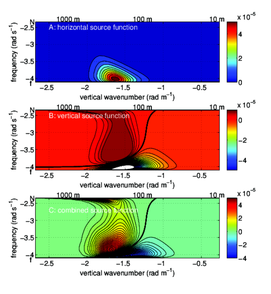

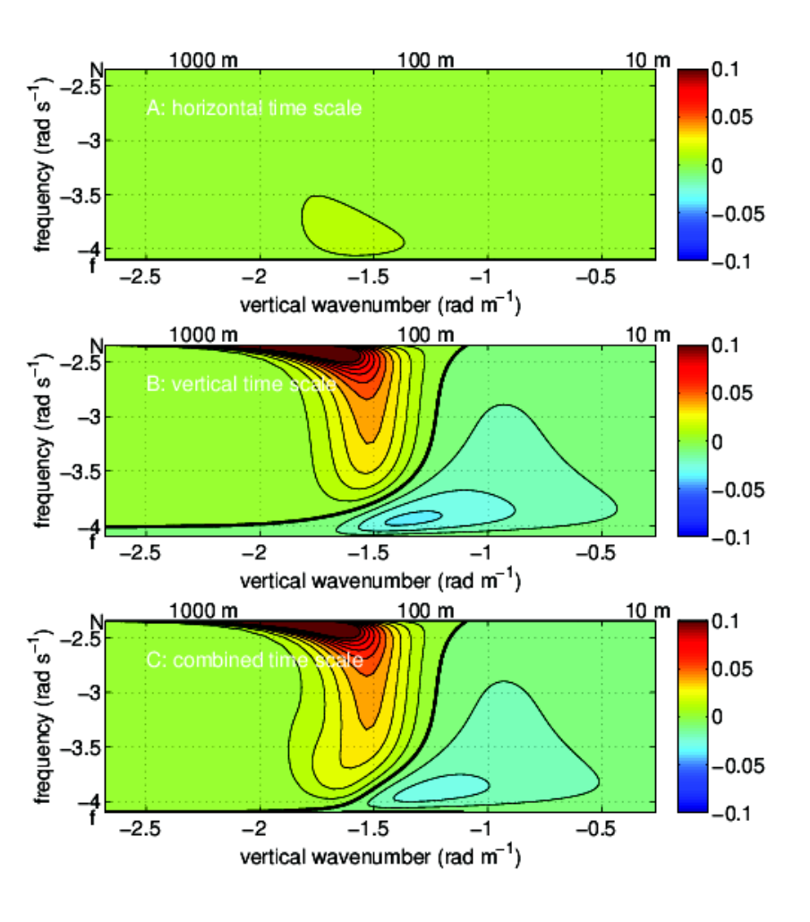
is required: such dynamics will compete with turning point effects and questions of how to specify in arise. Apart from the buoyancy frequency, note that these wave-mean transfers are far too small to offset resonant wave-wave interactions: Compare Fig. 38 with 43.
5.2.2 BudgetsEnergy exchange between the mean and wave fields results from a stress-strain relation in the horizontal. Direct evaluation of the energy exchange using the PolyMode LDE current meter array data (Polzin, 2010) returns a transfer rate somewhat smaller than previously obtained (Brown and Owens, 1981), W/kg at 825 m depth. If this value characterizes the thermocline region having a characteristic depth m, a net source strength of 0.4 mW m-2 can be anticipated, Table 1. This estimate may be biased low, however, as both vertical and horizontal velocity gradients increase towards the surface and the rate at which energy is transfered is proportional to the velocity gradient variances. The LDE was located at (N, W), midway between Lotus and Fasinex. The estimates of energy transfer through eddy-internal wave coupling at 825 m depth do not Figure 44: Map of surface eddy kinetic energy in units of m2 s-2. Contour intervals are m2 s-2.
|
![[Uncaptioned image]](1007.2113v2/EKE_Atlantic_GC.png)
appear to explain
the regional seasonal cycle of internal wave energy. There is,
however, a seasonal cycle in upper ocean fronts associated with
buoyancy forcing, e.g., Weller (1991). This upper ocean frontal regime is
characterized by an Froude (vertical gradient of horizontal
velocity divided by buoyancy frequency) and Rossby (relative vorticity divided by ) number
parameter regime (Pollard and Regier, 1992) which may support more
efficient energy transfers than the quasi-geostrophic regime at the
thermocline base.
5.3 ForcingThe focus of the previous subsections was the genesis of spectral structure. In Sections 5.3, 5.4 and 5.5 we focus more upon (i) whether the variability in spectral parameters represents the character of the forcing at the endpoints of the cascade / spectral boundaries, and (ii) whether the forcing is consistent with the direction and magnitude of energy transfers.5.3.1 Near-inertial wave generation by a variable wind stressWork done by the wind in generating inertial frequency mixed-layer motions has been the subject of several recent publications. Nearly-global maps Figure 46: Map of near-inertial wind input into the mixed layer in units of W/m2, (Alford, 2003).
|
![[Uncaptioned image]](1007.2113v2/Atlantic_forcing_GC.png)


| of this wind work using the Pollard and Millard (1970) damped-slab model are presented in Alford (2003); Watanabe and Hibiya (2002), Fig.s 46 and 47. The slab model is highly idealized. Using observations of the upper ocean response to atmospheric forcing and a more sophisticated mixed layer model, Plueddemann and Farrar (2006) describe how the slab model tends to overestimate inertial frequency wind work by a factor of two. Their estimates for the Lotus, Fasinex and Subduction field programs are given in Table 1. Similar estimates for Site-D are presented in Silverthorne and Toole (2009). Plueddemann and Farrar (2006) also note that other modeling investigations (Crawford and Large (1996); Skyllingstad et al. (2000)) imply that only a fraction of this work () may be available for near-inertial | internal wave generation as the other part is lost to viscous dissipation in the mixed layer for the resonant forcing conditions that dominate the revised transfer estimates. ’Best’ estimates of source strength in Table 1 incorporates this dissipation. The aforementioned work concerns only getting inertial energy into the mixed layer. Radiation of this energy into the stratified interior can be represented by invoking a Fourier decomposition of the slab model and mapping onto the internal wavefield using a linear model that includes the variation of the Coriolis parameter with latitude (D’Asaro et al., 1995). There are, however, unresolved issues: the linear model under estimates the initial rate at which energy leaves the mixed layer by and can not explain the evolution of the small vertical wavelength |
near-inertial field. Nonlinear interactions are held to be a primary candidate to explain the later (D’Asaro, 1995). For further consideration of near-inertial motions see Section 5.5.
5.3.2 Surface-internal wave coupling
Internal waves can also exchange energy with the surface wavefield, thereby implying a parametric dependence of source strength upon wind stress and possible seasonality. In the resonant interaction approximation, a pair of surface waves with nearly equal wavenumber and frequency can interact with an internal wave mode through a difference interaction, Watson et al. (1976); Olbers and Herterich (1978). Estimates of energy transfer are sensitive to the structure of the upper ocean buoyancy profile. Estimates (Watson, 1994) using climatological buoyancy profiles and seasonally averaged wind estimates return transfer rates of several tenths of a mW m-2 from the internal wavefield to the surface wavefield during summer months (Fig. 48) and at low latitudes during winter months (Fig 49). The high latitude transfer rates during winter are smaller. In contrast to these wind wave results, rapid transfers of energy from a narrow band ocean swell to the internal wavefield are possible (Watson, 1990) and remain to be quantified.
5.3.3 Internal wave coupling to mixed-layer turbulence
The coupling of surface and internal gravity waves is not the only possible source of high frequency internal wave energy. It has long been conjectured that mixed-layer turbulence can be coupled to the internal wavefield, Bell (1978). Observations presented in Wijesekera and Dillon (1991) reveal a narrow band internal wave response in the upper equatorial ocean at frequencies near the upper ocean stratification rate. Skyllingstad and Denbo (1994) point towards shear instability as a generation mechanism. It is unclear how this mechanism translates to a rotating system.
Polton et al. (2008) use large-eddy simulations of mixed-layer turbulence with a parameterization of Stokes drift forcing by a surface gravity wavefield. This forcing sets up Langmuir circulations and a inertial current oscillation is superimposed that advects the Langmuir cells relative to the stratified interior. Vertical circulations of the Langmuir cells excite high frequency internal waves having a phase velocity that matches the depth averaged mixed layer velocity.
Polton et al. (2008) estimate that energy and momentum are radiated at rates comparable to those associated with near-inertial wave radiation. These waves, however, are likely trapped within the highly stratified transition layer with either implications for mixing or for acting as a source of high frequency energy that can be transported to lower frequency via wave-wave interactions. Analysis of upper ocean data sets for a high frequency response on the time scale of the wind forcing could be quite enlightening.
5.3.4 Tides
Spatial Patterns
Numerical models have, in several instances, been used to both estimate the energy conversion from barotropic to baroclinic tides and keep track of the nonlinear evolution of the internal tides (e.g., Simmons (2008)). While such models may not have the spatial resolution required to get the details of the nonlinear transfer process right, or pick up the generation of baroclinic tides from small scale topographic roughness, they should give some indication of where the PSI decay can expected to be important. The eastern Atlantic is one such region, Fig. 50, providing further circumstantial evidence that the Natre spectrum is forced primarily through PSI decay.
Budgets The issue of internal tide generation, propagation and decay has received a great deal of attention this past decade, in part due to several major field programs (the Brazil Basin Tracer Release Experiment Ledwell et al. (2000) and the Hawaiian Ocean Mixing Experiment Rudnick et al. (2003)). Near global maps of the rate of conversion of barotropic tidal energy to baroclinic (internal) tidal energy have been provided by several Egbert and Ray (2003); Simmons et al. (2004); Simmons (2008); Niwa and Hibiya (2001) groups. As our focus is on the background internal wavefield, none of the data sets described here is from a region of significant barotropic to baroclinic conversion.

The relevant phenomena appears to be the far-field decay of a low-mode tide via resonant interactions. This particular phenomena is believed to be most important when the frequency of the low-mode tide is slightly higher than the Coriolis frequency, e.g., Furuichi et al. (2005). For , this corresponds to latitudes equatorward of . Many of the data sets examined here are in the vicinity of this critical latitude, particularly in the western North Atlantic. There, however, estimates suggest a low mode internal tide with horizontal energy flux of approximately 300 W m-1 (Hendry, 1977)66 6 Hendry’s estimate of 300 W/m to the south east represents a short term estimate from the MODE current meter array centered about N, W. Long term estimates from single moorings at N, W (LDE) and N, W (LOTUS) (Alford and Zhao, 2007) are approximately 150 W/m to the north-northwest and 200 W/m to the southeast. It is tempting to interpret energy flux estimates in Fig. 1 of Simmons (2008) as suggesting that the western boundary is a source of baroclinic tidal energy at these latitudes. The lack of consistency is troubling and the issue warrants further investigation. and analyses of relevant data from the western North Atlantic have not emphasized an interpretation of semidiurnal tidal PSI decay. An order of magnitude estimate of source strength as the observed flux distributed over the distance from the assumed source (the Blake Escarpment some 700 km distant) is smaller ( 300 W m-1 / 700 km) than the nominal background dissipation rate, O(1 mW m-2), Section 5.4. Moreover, the internal tide likely cannot explain the observed seasonal cycle in high frequency internal wave energy if the source has been correctly identified. Baines (1982) finds that the details of the stratification profile are important in estimating the rate of conversion of barotropic tidal to baroclinic energy, but the Blake Escarpment is a relatively deep feature and extends only to 1000 m water depth, well below seasonal changes in stratification.
Decay of a low mode-tide via resonant interactions poleward of the critical latitude would be through the induced diffusion mechanism. Olbers and Pomphrey (1981) argue that decay of a line spectrum with a typical energy density of 100 J m-2 would result in loss from the tides at rates between 0.005 to 0.05 mW m-2. Such values will not contribute significantly to the internal wave energy balance, but note: the calculation is based upon GM76, and with the estimate is biased.
Barotropic tidal velocities in the eastern North Atlantic are typically larger than in the west, and, consistently, available estimates of the low mode internal tide (Rossby (1988); Siedler and Paul (1991); Alford and Zhao (2007)) are typically larger. However, such estimates exhibit significant spatial and temporal variability. Preliminary estimates of internal tide parameters from the Subduction array’s center mooring assign rms buoyancy scaled velocities of (0.02,0.02) m s-1 and 4 m displacement to mode-1, and implying an energy flux of approximately 1 kW m-1. This is a surface mooring and contamination of energy flux estimates by vertical motion in response to ambient currents is a definite concern. Alford and Zhao (2007) present energy flux estimates of roughly 750 W/m for this mooring. This energy flux is directed to the northeast, seemingly at odds with both near-field and far-field sources (a minor seamount that rises to depths of 3000 m immediately to the east, the Great Meteor seamount to the north and the European continental shelf to the northeast). Energy flux vectors in Simmons (2008) are to the west.
An order of magnitude estimate of the flux divergence (Table 1) can be obtained by dividing 1 kW m-1 by the length scale characterizing the spatial variability in the internal tide amplitude, roughly 1,000 km.
| program | latitude | longitude | mechanism | start | stop | source strength |
|---|---|---|---|---|---|---|
| Lotus | 34∘N | 70∘W | wind work | May 1982 | Oct. 1982 | 1 mW m 50% |
| LDE | 31∘N | 70∘W | eddy-wave coupling | May 1978 | July 1979 | 0.4 mW m-2 |
| Mode | 28∘N | 70∘W | tide | March 1973 | July 1973 | 300 W m-1 / 700 km |
| Fasinex | 27∘N | 70∘W | wind work | Jan. 1986 | May 1986 | 0.4 mW m 50% |
| Subduction | 25.5∘N | 29∘W | wind work | April 1992 | Oct. 1992 | 0.05 mW m 50% |
| Subduction | 25.5∘N | 29∘W | tides | April 1992 | Oct. 1992 | 1 kW m-1 / 1000 km |
| Site-D | 39∘N | 69∘W | wind work | November 2001 | April 2006 | 1.0 mW m 50% |
5.4 Dissipation
Our underlying hypothesis is that the observed variability can be understood as spatially local stationary states of the radiation balance equation (26). In this context, the role of dissipation is possibly two fold. First, in a local stationary balance, forcing balances dissipation. Second, dissipation may play a role in actively shaping high wavenumber spectra. We take up these issues in turn below.
5.4.1 Budgets
Internal wave energy can be dissipated in the interior through wave breaking and at the boundaries as work done against viscous stresses.
Depth integrated dissipation rates in the open ocean will typically exceed dissipation in the bottom boundary layer, D’Asaro (1982); Fu (1981). The contribution of the bottom boundary layer is mitigated by buoyancy scaling of internal wave velocity and low stratification in the abyss. Away from regions of topographic generation, dissipation associated with interior wave breaking is dominated by thermocline and upper ocean regions having large stratification rates. One atypical example in which boundary layer dissipation can dominate is under ice cover in the Canadian Basin of the Arctic Ocean. There, the internal wavefield is anomalously weak and buoyancy scaling implies internal wave velocities are largest near the upper boundary. A second atypical example is in regions of large geostrophic currents in which wave dissipation can be modeled through a linearization of the bottom stress (Polzin, 2010).
Interior wave breaking is usually conceived of as a high wavenumber sink associated with instability mechanisms, e.g., Polzin (1996). That sink represents a production term in a turbulent mechanical energy budget:
| (76) |
being balanced by a buoyancy flux and dissipation and a stochastic production/dissipation balance. The correlations inherent in both production and buoyancy flux terms are difficult to measure directly. Rather, specialized instrumentation and platforms are used to estimate the rate of dissipation . Full-depth estimates of such microstructure data are limited. In its stead, use has been made of finestructure parameterizations based upon (70). These assign a value of
to GM76 at 30 degrees latitude and a buoyancy frequency of 3 cph.
With either fine- or microstructure method, a major caveat is that one needs to understand how (not just whether) the sampling of the wavefield is biased. For example, while one might hope to make sense of observations in NATRE as being almost exclusively forced by a PSI decay (Polzin et al., 2008), analysis of the diapycnal dispersion of an anthropogenic tracer suggests a long term average of a factor of two larger. The difference may actually be related to the spatial variability of the tide. Experience (Polzin, 2009) suggests that issues of biasing in regions of rough topography are much more problematic than the factor of two in NATRE.
5.4.2 Spectral Patterns: models
In order to reconcile the high wavenumber normalized Boltzman rates with the claim that GM76 represents a stationary state, McComas and Müller (1981b) invoke a spectral representation that assumes dissipation events have space-time scales much smaller than the scales of the internal waves and that the turbulence can be parameterized by an eddy viscosity , resulting in
| (77) |
Similar representations are examined in greater detail in Natarov and Müller (2005).
Some generalization of this model may be required if it is necessary to invoke dissipation in order to obtain a stationary state. Dissipation events will typically have vertical scales smaller than the nominal 10 meter cut-off, gauged either by correlation length scales of turbulent dissipation (Gregg et al., 1993) or the exclusive contribution of sub-10 meter wavelength shear to the occurrence of supercritical Richardson number events (Polzin, 1996) (with supercritical Richardson number being indicative of shear instability), so the spatial scale separation between waves and turbulence could be justified. But the application of phenomenological mixing models indicates that dissipation events have lifetimes in excess of a buoyancy period (Polzin, 1996) so that a temporal scale separation is problematic. In general, Polzin (1996) finds such phenomenological mixing models to be useful diagnostic tools, but difficult to develop into prognostic models because of this finite lifetime.
A key point in a generalized model is that the finestructure parameterization (70) weights the contribution of each frequency to dissipation as a product of vertical gradient variance and aspect ratio and thus the contribution of high frequency waves. The dissipation function (77) weights each frequency only as the vertical gradient variance and so emphasizes the near-inertial that dominate the vertical shear. Phenomenological mixing models (Polzin, 1996) have been shown to be in agreement with (70). Observations presented in Alford and Pinkel (2000) also appear to support the role of high frequency variability.
A qualitative distinction between (77) and (70) may be drawn by noting that (77) is likely to be appropriate for a system of coupled oscillators. It may not make sense for a description of the internal wavefield as a system of wavepackets in which dissipation events are associated with the transport of individual wave packets to breaking scales, as invoked in the ray tracing models, e.g., Henyey et al. (1986). The ray-tracing model does not need a dissipation function because the wave packets are followed as particles to their annihilation.
We regard the impact of dissipation on the internal wave spectral domain as an open question awaiting rigorous analysis.
5.4.3 Spectral Patterns: The mid-frequency dip and bottom boundary conditions
Many of the frequency spectra are poorly characterized by a simple power law fit near semidiurnal frequencies (e.g., Fig. 13). Apart from the tidal peak, observed spectral levels tend to be smaller than the power law characterization. Levine (2002) forwards the hypothesis that this mid-frequency dip is related to nonlinearity in how energy is transfered to higher and lower frequency out of the semidiurnal peak. Here we forward an additional hypothesis regarding such departures. With a buoyancy profile that decreases towards the bottom boundary, only the low frequency portion of the wavefield reaches the bottom, where wave energy can be dissipated as work done against viscous stresses and vertical scale transformations associated with reflection or scattering from a nonuniform bathymetry can act. Calculations have already been made to assess the rate at which energy is redistributed by such scale transformations for the GM spectrum, e.g., (Müller and Xu, 1992; Eriksen, 1985b). With an eye toward explaining spatial variability of the background spectrum, one can also ask the question of how the equilibrated spectrum could be shaped by the cumulative effects of scale transformations acting through the bottom boundary condition and nonlinearity acting through radiation balance equation’s source function. This is a topic for future research, which requires a relatively sophisticated treatment of (26).
5.5 Propagation
The ability of low mode internal waves to propagate long distances from their generation sites is loosely constrained in the observational record and is a serious issue for internal wave energy balance studies. The most significant processes are tidal constituents and near-inertial waves. These internal waves do not play a major role in this Regional study of the high wavenumber / high frequency spectral variability. They do, however, act as sources for the internal wave continuum, whether it be through extreme scale separated interactions (Section 5.1.1.c) or via a PSI decay process of tidal energy into near-inertial waves that then is linked to the continuum (Section 5.1.2).
We anticipate that variability in the tidal and inertial peaks is linked to variability in the continuum. Fu (1981) documents variability of the inertial peak in the Western North Atlantic and obtains the following Regional classification scheme: Class 1 spectra have prominent inertial peaks. Such spectra occur in records obtained from the Mid-Atlantic Ridge in the vicinity of N and occur in conjunction with relatively white frequency spectra. We anticipate that the inertial peaks here are related to a PSI decay process (Section 5.1.2.a). Class 2 spectra have less prominent peaks and are found (a) in the upper ocean at depths less than 2000 m, (b) in the deep ocean above rough topography off the Mid-Atlantic Ridge axis and away from N and (c) in the deep ocean under the Gulf Stream. We anticipate issues of internal lee-wave generation and wave-mean interactions (Section 5.2) to be significant. Finally, Class 3 spectra have the smallest inertial peaks and are found above smooth topography. Fu (1981) argues that Class 1 and Class 2 inertial peaks are associated with local processes and Class 3 inertial peaks are consistent with propagation effects as waves initialized with the GM76 spectrum reflect from their turning latitudes. Such quantitative estimates depend upon the vertical modal distribution of energy, and the regional variability of is not well constrained in that study. Fu (1981)’s study included the MODE Central mooring instrumented at [500 (class 2a), 1500(class 2a), 4000(class 3)] m depth, whose location was the site of moorings during IWEX and FASINEX, Section 3.3.2; and PolyMode IIIc mooring 82 [172(class 2a), 322(class 2a) 522 (class 2a), 2446 (class 2b), 3946 (class 2b)], Section 3.3.3. The vertical profile data sets at these locations in our study are focused upon depths less than 2000 m. Leaman (1976), however, comments upon differences between vertical profiles obtained over rough and smooth topography in the vicinity of MODE Central.
The last decade has seen the development of General Circulation Models that include both tidal forcing and wind products with sufficient temporal resolution to force inertial motions (Simmons, 2008; Arbic et al., 2010). The models, however, obey their own dynamics: near-inertial forcing will be influenced by the mixed layer scheme, absence of an eddy field, presence/absence of a realistic internal wavefield, topographic representation, sub-grid closures, etc. Unraveling how such model fields relate to the ocean will be a complicated, but useful aid in interpreting the oceanic internal wavefield.
The issue of propagation demands careful assessment. As long as the roles of the bottom boundary condition and refraction in the mesoscale eddy field are not appreciated, the dominant balance of terms in an energy budget can seriously be misconstrued. See, for example, the difference of opinion about the Brazil Basin data set in St.Laurent and Garrett (2002) and Polzin (2004b) that appears to be resolved in favor of a high efficiency of topographic scattering in Polzin (2009).
Similarly, Alford and Zhao (2007) estimate significant horizontal energy fluxes in the near-inertial band north of the Gulf Stream and regard those flux estimates as symptomatic of the ability of low-mode waves to propagate large distances. The issue of mooring motion contaminating the horizontal energy flux estimates bears further investigation before those flux estimates can be considered robust.
6 Conclusion
The ingredients that shape the deep ocean energy spectrum have been known for some time. Fig. 34 from McComas (1977) presents one version of how these ingredients can be combined. In that recipe, the primary sources are at high frequency and a transfer of energy to higher vertical wavenumber is associated with the ID mechanism. Parametric spectral fits summarized in Fig. 37 are highly suggestive that the ID mechanism plays an active role in determining the observed power laws. However, the details are not consistent with such an interpretation.
We now believe that near-inertial and tidal sources dominate high frequency sources of internal wave energy, and this posses a real challenge to the induced diffusion mechanism: Energy transports associated with induced diffusion are to higher vertical wavenumber and lower frequency for vertical wavenumber domain power laws . That requires a source of high frequency energy. Possible sources are coupling of internal waves with surface swell, internal wave coupling to mixed layer turbulence and a weaker version of internal wave coupling to the eddy field. These possible sources are not well constrained, either observationally or theoretically.
A second facet is that transports under the resonant interaction approximation are not completely understood. Hitherto neglected local interactions may play a significant role in determining nonlinear transports.
A third facet is that resonant kinetic equation evaluations in Fig. 40 indicate GM76 is far from being a stationary state, seemingly at odds with GM76 representing an ID no flux state. Self-consistent solutions to a broadened kinetic equation could be much closer to being stationary and exhibit energy transfers appropriate for low frequency sources. A closely related result is that ray-tracing diagnostics imply a transport of action to higher frequency. This transport could provide a pathway to supply energy to the high wavenumber continuum. A first principles derivation of the spectral transports associated with the ray-tracing models would be enlightening.
Despite such uncertainty, nonlinearity is clearly an organizing principle. Power laws associated with parametric spectral representations lie close to the Induced Diffusion stationary states of the resonant kinetic equation describing the lowest order nonlinear transfers. The one exception appears to be a wavefield set up by the decay of a semidiurnal internal tide through the parametric subharmonic instability.
While our ideas of the ingredients and their geographic distribution has evolved, our knowledge of how to create the observed spectrum (the recipe) has remained relatively static. We are confident that such recipes are within reach, but it will take a combination of observations, analytic work in the context of a radiation balance equation and realistic direct numerical simulations. Theoretical studies coupled to observational programs, especially those that would document 2-D spectra, transfer rates, the spectral character of the forcing functions and seek to define the role of the geostrophic flow field are a high priority. Resonant calculations show strong non-stationary tendencies, and this issue needs to be either resolved or circumvented before addressing the contributions of other ingredients to the recipes.
Regionality
Variability in the spectral characteristics of the deep ocean internal wavefield documented in Section 3 and consideration of regional variability in the forcing fields in Section 5 leads us to propose the following strawmen for further investigation:
- •
The Natre region is a minimum for eddy energy in the North Atlantic and wind work at near-inertial frequencies is small. Equatorward of the critical latitude for tides, PSI decay of the low-mode internal tide represents the major forcing of the internal wavefield. The Natre spectrum is an outlier with extremely high bandwidth, steep vertical wavenumber and shallow frequency spectral slopes. A preliminary recipe for the Natre region is described in Section 5.1.2.a. This recipe invokes a heuristic cascade closure for nonlinearity that has its roots in the ray-tracing diagnostics.
- •
The contrasts between the wavefields north and south of the Gulf Stream are distinct and appear to have a parallel with differences between subtropical and subpolar gyres in the North Pacific along its eastern boundary. The later case deserves further investigation to confirm spectral parameters graphically extracted from the literature. Our leading hypothesis is that the differences can be directly related to the relative roles of near-inertial wind forcing and interactions with the mesocale eddy field via (74) and (75). We have not yet translated this hypothesis into a recipe.
- •
The tentative signature of a phase lag between seasonal cycles in high frequency and near-inertial frequency waves in the eddy desert of the North Pacific may be a signature of nonlinear transfers in the absence of wave-mean coupling.
The future will certainly bring many further exciting developments, and the synthesis of theoretical, observational and numerical results yet to be obtained.
Appendix A Meta data
| place | latitude | longitude | water depth | sensor depth | inst. type | code | start | stop | cph | C/m |
| Site-D | 39 | 70 | 2640 m | 106 | VACM | WHOI 2203 | Feb. 26, 1967 | Mar. 25, 1967 | 3.03 | |
| 511 | WHOI 2204 | 1.48∗ | ||||||||
| 1013 | WHOI 2205 | 0.66∗ | ||||||||
| 1950 | WHOI 2206 | 0.58∗ | ||||||||
| Shelf-Slope | 39 | 70 | 2305 m | 305 | VACM | WHOI 5881 | Feb. 10, 1976 | Aug. 8, 1976 | 2.82∗ | -0.0235∗ |
| Primer | 39 | 69 21.4′ | 2990 m | 391 | VACM | WHOI 9872 | Dec. 8, 1995 | Dec. 4, 1997 | 2.39∗ | -0.0170∗ |
| Iwex | 27 | 69 50.95′ | 5453 m | 604 | VACM | WHOI 515A4 | Nov. 3, 1973 | Dec. 15, 1973 | 2.55 | -0.0175 |
| 604 | VACM | WHOI 515B4 | Nov. 3, 1973 | Dec. 15, 1973 | 2.55 | -0.0177 | ||||
| 633 | VACM | WHOI 515C5 | Nov. 3, 1973 | Dec. 15, 1973 | 2.60 | -0.0157 | ||||
| Lotus | 34 1.2 | 70 1.45 | 5366 | 328 | VACM | WHOI 7666 | May 11, 1982 | April 12, 1983 | 1.49 | -0.00356 |
| 33 58.55 | 70 0.36 | 5366 | 348 | VACM | WHOI 7886 | April 14, 1983 | May 1, 1984 | 1.49 | -0.00356 | |
| PolyMode III-c | 15 23.40 | 53 55.20 | 319 | VACM | NOVA 80 | May 11, 1977 | May 1, 1978 | 2.78 | -0.03096 | |
| 15 11.50 | 53 12.30 | 309 | VACM | NOVA 81 | May 12, 1977 | Dec. 20, 1977 | ||||
| 15 02.10 | 54 12.90 | 338 | VACM | NOVA 82 | May 13, 1977 | May 1, 1978 | ||||
| Fasinex | 27 58.9 | 69 58.8 | 556 | VACM | WHOI 8293 | Oct. 29, 1984 | June 18, 1986 | 2.48 | -0.0178 | |
| 631 | VACM | WHOI 8294 | 2.61 | -0.0202 | ||||||
| Subduction | 25 31.90 | 28 57.2 | 300 | VMCM | WHOI | Feb. 12, 1992 | Oct. 14, 1992 | 2.44 | -0.02244 | |
| Subduction | 25 31.90 | 28 57.2 | 300 | VMCM | WHOI | Oct. 15, 1992 | June 16, 1993 | 2.44 | -0.02244 | |
| EBC | 37 6.7 | 127 32.1 | 4752 | 598 | Aanderaa | rcm02674 | Aug. 9, 1992 | Aug. 19, 1994 | 2.01 | 0.00455 |
| Ocean Storms | 47 25.4 | 139 17.8 | 4224 | 199 | VMCM | rcm07420 | Aug. 20, 1987 | June 25, 1988 | 2.25 | 0.006 |
| AIWEX | 74 | 143-144 | 3700 | 250 | SBE-3 | - | Mar. 20, 1985 | Apr. 5, 1985 | - | 0.02 |
| place | latitude | longitude | water depth | inst. type | start | stop |
|---|---|---|---|---|---|---|
| Station-W(3) | 39 | 70 | 3000 | MMP | Jun. 20, 2003 | Aug. 5, 2003 |
| Station-W(3) | 39 | 70 | 3000 | MMP | Jan. 17, 2004 | Mar. 2, 2004 |
| Mode | 28 | 69 40′ | 5440 | EMVP | Jun. 11, 1973 | Jun. 15, 1973 |
| Fasinex | 27-29 | 67 - 70 | 5200 | HRP | Feb. 17, 1986 | Mar. 5 1986 |
| Natre | 23 - 27 | 26 - 30 | 5500 | HRP | Mar. 28, 1992 | Apr. 14, 1992 |
| SFtre2 | 14-16 | 50-57 | 5400 | HRP | Nov. 14, 2001 | Nov. 24, 2001 |
| Patchex1 | 34 | 127 | 4700 | MSP | Oct. 17, 1986 | Oct. 24, 1986 |
| Patchex2 | 34 | 127 | 4700 | FLIP | Oct. 1986 | 7.5 days |
| Swapp | 35 8.2′ | 126 59.0′ | 4700 | FLIP | Feb.-Mar. 1990 | 18 days |
| STREX | 50 | 140 | 4000 | XCP | Nov. 8 1980 | Nov. 22, 1980 |
| AIWEX | 74 0′ - 74 12′ | 144 - 145 | 3750 | XCP | April 3, 1985 | April 14, 1985 |
Appendix B Instrumentation
A terse presentation of many of these data was made in Lvov et al. (2004), simply summarizing the available power law estimates as points in a frequency-wavenumber domain. That presentation was limited to spectra appearing in published literature. The intent of this work was to present pertinent data in a common framework, limiting the potential pitfalls associated with an irregular analysis. This does not limit uncertainties associated with the use of different instrument systems. Details of an instrumental and technical nature that impact the interpretation of the data are collected herein.
B.1 Moored Current Meters
Regarding the interpretation of moored current meter data as internal waves, there are two primary sets of issues. The first set is referred to as finestructure contamination. Here the presumption is that the data record represents signal and that departures from linear internal wave kinematics are associated with either: (a) quasi-permanent finestructure (either density or velocity) being advected past the sensor (e.g., Polzin et al. (2003), 2.1.4), (b) self-advection within the wavefield (e.g., Sherman and Pinkel (1991), 5.1.4), or (c) attempting to estimate density perturbations using temperature data only and invoking a stable relation between density, temperature and salinity. This later assumption fails in regions that have significant large-scale gradients of temperature and salinity on isopycnals (e.g., Ferrari and Polzin (2005)). See the cited references for further discussion of these issues. The second set of issues are instrumental in nature: (a) drag associated with flow past a mooring will induce movement (e.g., Foffonoff (1966)), (b) typical sampling rates are not sufficient to resolve internal wave spectrum out to the buoyancy frequency in the upper ocean, and (c) instrument response issues.
Regarding (a), there are typically 3 classes of moorings: deep, intermediate and surface. A deep mooring will utilize glass balls as buoyancy elements distributed along the mooring cable. The primary buoyancy element for an intermediate mooring will be a large syntactic sphere at the upper terminus. This mooring type utilized at WHOI starting in the early 1980’s. It has less over all drag and consequently provides a more stable platform. Finally, surface moorings are loosely tethered in order to accommodate the often sizable surface motions associated with surface waves. As a result, the surface buoy inscribes a watch circle roughly equal to the water depth (Trask et al., 1982). Vertical motion of the instruments can be diagnosed if pressure sensors are included, e.g., Fig. 51. Experience suggests inertial and tidal frequencies suffer greater contamination by mooring motion than super-tidal frequencies. Significant discussions appear in Fu (1981) and Ruddick and Joyce (1979).
Regarding (b), insufficient sampling rates rates will result in the aliasing of high frequency signals back into the resolved frequency domain. Ordinarily, the frequency spectra will be sufficiently red that the aliased energy is relatively small. However, if there is a substantial bump at the buoyancy frequency associated with turning point dynamics (e.g., Desaubies (1975)), the aliased energy may be significant. Ascertaining whether this is the case requires information on the vertical wavenumber content of the wavefield and details of the vertical structure of the buoyancy profile. Without such information and in the absence of pressure records, it is difficult to assert that the departure of the observed high frequency spectra in Fig. 2, for example, are noise rather than signal.
Regarding (c), the principle moored current meters used here are the Vector Averaging Current Meter (VACM) and Vector Measuring Current Meter (VMCM). The VACM employs a Savonius rotor and the VMCM uses sets of propellors. The VMCM (Weller and Davis, 1980) was designed to have a cosine response to eliminate ‘pumping’ associated with the motion of a surface mooring. VACMs are standard for subsurface moorings. VACMs have a finite stall speed of about 2 cm s-1 (Luyten and Stommel, 1991). Good directional data is believed to be obtained at speeds smaller than this. The resulting ‘noise’ is not well defined. VMCM data are calibrated assuming no significant stalling. See Hogg and Frye (2007) for a more recent discussion of current meter performance.

B.2 Doppler Sonars
Doppler sonars do not measure horizontal velocity as a point but determine Doppler shifts as a function of range along multiple acoustic beams. These Doppler shifts are interpreted as slant velocities of suspended acoustic backscattering targets moving with the water relative to the instrument platform. Individual estimates of ocean velocity are highly uncertain: hundreds of pings are typically used to average incoherent noise from the system. Estimates of signal-to-noise ratios appear in Anderson (1992) and an appendix of Alford and Pinkel (2000). The insidious complication of package motion and beam separation effects are considered in Polzin et al. (2002).
B.3 Vertical Profiling Instrumentation
Most of the vertical wavenumber domain information considered here was obtained with vertical profiling instrumentation. Estimates of the vertical structure of the velocity field can be obtained by using a number of different sensors, each of which with its own strengths and weaknesses.
Sanford’s ElectroMagnetic Velocity Profiler (EMVP, Sanford (1975)) senses the voltage drop associated with an electrical current (seawater) in a magnetic field (the Earth’s, in this case). The measurement is uncertain to within a conductivity weighted mean, so that other sensors need to be incorporated to provide estimates of the absolute velocity field. Noise levels are typically around 0.5 cm s-1, which is sufficient to start resolving vertical wavelengths smaller than 10m. Expendable Current Profilers (XCPs) operate on the same principle, but may have somewhat larger noise levels (1.0 cm s-1).
Data from several acoustically tracked dropsonde’s have been analyzed but not presented. With this instrument system, the horizontal position is estimated from range information provide by an acoustical net and depth information from an onboard CTD (Conductivity-Temperature-Depth sensor suite). Oceanic velocity estimates assume that the package tracks the flow field as it descends. This method provides estimates of the absolute velocity, but the small scale noise is relatively high. Acoustic tracking provides positions to within 1 m. A typical descent rate of 1 m s-1 implies that the background internal wavefield having vertical wavelengths smaller than several hundred meters will be obscured by noise.
A third method is to utilize an acoustic travel time sensor to estimate relative flow past a freely-falling vehicle [e.g., the High resolution Profiler (Schmitt et al., 1988) and the Multi-Scale Profiler (Winkel et al., 1996)]. Estimates of the oceanic velocity profile are deduced from these relative velocity data and a model of how the vehicle responds to the relative flow. The method is capable of resolving oceanic shear at 1-m scales. The limitations are at larger wavelengths. The offsets (zeros) of the acoustic travel time sensor are typically determined in situ and may even be temperature and pressure dependent. Thus the resulting profiles are uncertain to a linear trend. Other information, such as provided by an electric field sensor or matching with a shipboard ADCP record, are required to provide the largest scale information.
Acoustic travel time sensors are used in the McClane Moored Profiler (MP, Doherty et al. (1999)). This instrument autonomously samples relative velocity, temperature, conductivity and pressure while transiting a mooring cable. Estimates of relative velocity are thus absolute. Noise levels in the velocity record are nominally estimated at 0.5 cm . Biases related to drifting zeros and mooring oscillations are not presently well defined.
Velocity data obtained with Doppler sonars typically estimate horizontal velocity from back-to-back acoustic beams. In so doing, one assumes that the velocity field is horizontally uniform. This assumption breaks down as the beam separation increases and will preferentially contaminate high frequency, small vertical scale signals. Polzin et al. (2002).
Appendix C Processing
In the absence of a mean flow, the linear internal wave equation is (e.g., Gill (1982)):
| (78) |
for arbitrary stratification profile and vertical velocity . If the stratification profile varies much more slowly than the wave phase, a WKB approximation for vertically propagating waves provides the approximate solution:
| (79) |
and so the effects of a variable buoyancy profile can be accounted for by stretching the depth coordinate by and scaling the horizontal velocities by , in which is a reference stratification. The value 3 cph is often used. The use of the WKB approximation requires . If this relation is not satisfied, solutions can be found by treating (78) as an eigen value problem with appropriate boundary conditions. If but the wave-phase is not slowly varying, the boundary conditions are that at the top () and bottom (), which then implies the horizontal velocities are proportional to:
| (80) |
for integer values of n. For data sets that document the velocity profile over the entire water column, the first three modes have been estimated by using a linear regression. Vertical wavenumber spectra are calculated by using a cubic spline to interpolate onto a uniform grid having approximately the same resolution as the unstretched data.
Current meter data used here have sampling intervals of 3.75 minutes to 1 hour. Frequency spectra have been calculated using transform intervals of and days. Spectra are displayed using the later at super-tidal frequencies ( / cpd) and the former at lower frequencies. The intent is to give finer resolution to inertial and tidal peaks and decreased variability at higher frequency.
Appendix D A Sargasso Sea spectrum
We have characterized the background internal wave spectrum in the Sargasso Sea as:
| (81) |
with m-1 and normalization constant chosen to return m2 s-2. This places the gradient variance at approximately . Power laws are characteristic of the Sargasso Sea Data sets (Section 3.3.2) are selected specifically to lie on the Induced Diffusion constant flux solution (Section 5.1.1.c). The inertial peak was selected with the constraint that based upon moored data. We have deferred from invoking non-separable conditions via that are a documented part of the observational record (Müller et al., 1978) and appear as in excess of this value (Polzin et al., 2003).
Acknowledgements.
The authors gratefully acknowledge the efforts of many talented researchers who were instrumental in collecting, processing and archiving the data presented here. Special thanks are extended to John Toole for providing yet unpublished MP data from Site-D, Tom Sanford for providing access to a number of his EMVP and AVP data sets, and to Carl Wunsch for the PolyMode IIIc current meter data set. We greatfully acknowledge funding provided by a Collaborations in Mathematical Geosciences (CMG) grant from the National Science Foundation.References
- Anderson (1992) Anderson, S. P. (1992), Shear, Strain and Thermohaline Fine Structure in the Upper Ocean. Ph.D. Thesis, UCSD, pp. 173.
- Alford and Pinkel (2000) Alford, M. (2000), Observations of Overturning in the Thermocline: The Context of Ocean Mixing. J. Phys. Oceanogr., 30, 805–832.
- Alford (2003) Alford, M. (2003), Improved global maps and 54-year history of wind-work on ocean inertial motions. Geophys. Res. Lett., 30, doi:10.1029/2002GL016614.
- Alford and Whitmont (2007) Alford, M. H. and M. Whitmont (2007) Seasonal and spatial variability of near-inertial kinetic energy from historical moored velocity records. J. Phys. Oceanogr., 37, 2022–2037.
- Alford and Zhao (2007) Alford, M. H. and Z. Zhao (2007) Global Patterns of Low-Mode Internal-Wave Propagation. Part I: Energy and Energy Flux. J. Phys. Oceanogr., 37, 1829–1848.
- Arbic and Flierl (2004) Arbic, B. K. and G. R. Flierl (2004), Effects of mean flow direction on energy, isotropy, and coherence of baroclinically unstable beta-plane geostrophic turbulence. J. Phys. Oceanogr., 34, 77–93.
- Arbic et al. (2010) Arbic, B. K., A. J. Wallcraft and E. J. Metzger, Concurrent simulation of the eddying general circulation and tides in a ocean model. Ocean Modelling, 32, 175–187.
- Baines (1982) Baines, P. G. (1982), On internal tide generation models. Deep-Sea Res., 29, 307–338.
- Bell (1978) Bell, T. H. (1978), Radiation damping of inertial oscillations in the upper ocean, J. Fluid Mech., 88, 289–308.
- Bender and Orzag (1978) Bender, and Orzag (1978), Advanced Mathematical Methods for Scientists and Engineers. McGraw-Hill, New York, pp. 593.
- Blumsack (1993) Blumsack, S. L. (1993), A model for the growth of mudwaves in the presence of time varying currents, Deep Sea Res. II, 40, 963–974.
- Briscoe (1975a) Briscoe, M. G. (1975a), Internal waves in the ocean. Rev. Geophys. and Space Phys., 13, 591–598.
- Briscoe (1975b) Briscoe, M. G. (1975b): Preliminary results from the trimoored internal wave experiment (IWEX). J. Geophys. Res., 80, 3872–3884.
- Briscoe and Weller (1984) Briscoe, M. G. and R. A. Weller (1984), Preliminary results from the long-term upper-ocean study (LOTUS). Dyn. Atmos. Oceans, 8, 243–265.
- Brown (1974) Brown, N. L. (1974), A precision CTD microprofiler. Ocean 74, 2, 270-278.
- Brown and Owens (1981) Brown, E. D. and W. B. Owens (1981), Observations of the horizontal interactions between the internal wave field and the mesoscale flow. J. Phys. Oceanogr., 11, 1474–1480.
- Bühler and McIntyre (2005) Bühler, O. and M. E. McIntyre (2005), Wave capture and wave-vortex duality. J. Fluid Mech., 534, 67–95.
- Cairns (1975) Cairns, J. L. (1975), Internal wave measurements from a midwater float. J. Geophys. Res., 80, 299–306.
- Cairns and Williams (1976) Cairns, J. L., and G. O. Williams (1976), Internal wave observations from a midwater float. 2. J. Geophys. Res., 81, 1943–1950.
- Carnevale and Frederiksen (1983) Carnevale G. F. and J. S Frederiksen (1983), A statistical dynamical theory of strongly nonlinear internal gravity waves. Geophys. Atrophys. Fluid Dynam., 33, 175–207.
- Chereskin et al. (2000) Chereskin, T. K. , M. Y. Mooris, P. P. Niiler, P. M. Kosro, R. L. Smith, S. R. Ramp, C. A. Collins and D. L. Musgrave (2000), Spatial and temporal characteristics of the mesoscale circulation of the California Current from eddy-resolving moored and shipboard measurements. J. Geophys. Res., 105 (1245–1269).
- Crawford and Large (1996) Crawford, G. B. and W. G. Large (1996), A numerical investigation of resonant inertial response of the ocean to wind forcing. J. Phys. Oceanogr., 26, 873–891.
- Codiga and Eriksen (1997) Codiga, D. L. and C. C. Eriksen (1997), Observations of low frequency circulation and amplified subinertial currents at Cobb seamount. J. Geophys. Res., 102, 22993–23007.
- Doherty et al. (1999) Doherty, K.W., D.E. Frye, S.P. Liberatore and J.M. Toole (1999), A moored profiling instrument. J. Atmos. Oceanic Tech., 16, pp. 1816Ð1829,
- D’Asaro (1982) D’Asaro, E. A. (1982), Absorption of internal waves by the benthic boundary layer. J. Phys. Oceanogr., 12, 323–336.
- D’Asaro (1984) D’Asaro, E. A. (1984), Wind forced internal waves in the North Pacific and Sargasso Sea. J. Phys. Oceanogr., 14, 781–794.
- D’Asaro (1985) D’Asaro, E. A. (1985), The Energy Flux from the Wind to Near-Inertial Motions in the Surface Mixed Layer. J. Phys. Oceanogr., 15, 1043–1059.
- D’Asaro et al. (1995) D’Asaro, E. A. (1995), A collection of Papers on the Ocean Storms Experiment, J. Phys. Oceanogr., 25, 2817–2818.
- D’Asaro (1995) D’Asaro, E. A. (1995b), Upper-ocean inertial currents forced by a strong storm. Part II: Modeling, J. Phys. Oceanogr., 25, 2937–2952.
- D’Asaro and Morehead (1991) D’Asaro, E. A., and M. D. Morehead (1991), Internal waves and velocity finestructure in the Arctic Ocean, J. Geophys. Res., 96, 12725–12738.
- D’Asaro et al. (1995) D’Asaro, E. A., C. C. Eriksen, M. D. Levine, P. Niiler, C. A. Paulson, and P. Van Meurs (1995), Upper ocean inertial currents forced by a strong storm. Part I: Data and comparisons with linear theory. J. Phys. Oceanogr., 25, 2909–2936.
- Desaubies (1975) Desaubies, Y. J. F. (1975), A linear theory of internal wave spectra and coherences near the Väisälä frequency. J. Geophys. Res., 80, 895–899.
- Desaubies (1976) Desaubies, Y. J. F. (1976), Analytic representation of internal wave spectra, J. Phys. Oceanogr., 6, 976-981.
- DeWitt and Wright (1982) DeWitt, R. J. and J. Wright (1982), Self-consistent effective-medium theory of random internal waves. J. Fluid Mech., 115, 283–302.
- DeWitt and Wright (1984) DeWitt, R. J. and J. Wright (1984), Self-consistent effective-medium parameters for oceanic internal waves. J. Fluid Mech., 146, 253–270.
- Egbert and Ray (2003) Egbert, G. D. and R. D. Ray (2003), Semi-diurnal and diurnal tidal dissipation from TOPEX/Poseidon altimetry. Geophys. Res. Lett., 30 (1907) doi:10.1029.2003GL017676.
- Eriksen (1985a) Eriksen, C. C. (1985a), Some characteristics of internal gravity waves in the equatorial Pacific, J. Geophys. Res., 90, 7243–7255.
- Eriksen (1985b) Eriksen, C. C. (1985b), Implications of ocean bottom reflection for internal wave spectra and mixing. J. Phys. Oceanogr., 15, 1145–1156.
- Eriksen et al. (1991) Eriksen, C. C., R. A. Weller, D. L. Rudnick, R. T. Pollard and L. A. Regier (1991), Ocean frontal variability in the frontal air-sea interaction experiment, J. Geophys. Res., 96, 8569-8591.
- Ferrari and Polzin (2005) Ferrari, R., and K. Polzin (2005). Finescale variability of the T-S relation in the eastern North Atlantic. J. Phys. Oceanogr., 35, 1437–1454.
- Flatté et al. (1985) Flattè, S. M., F. S. Henyey and J. A. Wright (1985), Eikonal calculations of short-wavelength internal-wave spectra, J. Geophys. Res, 90, 7265–7272.
- Foffonoff (1966) Foffonoff, N. P. (1966), Oscillation modes of a deep sea mooring, Geo-marine Tech., 2, 13-17.
- Foffonoff (1969) Foffonoff, N. P. (1969). Spectral characteristics of internal waves in the ocean, Deep Sea Res., Suppl. to 16, 58-71.
- Fritts et al. (2003) Fritts, D.C. and Alexander M.J., Review of Geophys, 41, 10.1029/2001RG000106 (2003).
- Fu (1981) Fu, L. L. (1981), Observations and models of inertial waves in the deep ocean. Rev. Geophys. Space Phys., 19, 141–170.
- Furue (2003) Furue, R. (2003), Energy transfer within the small-scale oceanic internal wave spectrum. J. Phys. Oceanogr., 33, 267–282.
- Furuichi et al. (2005) Furuichi, N., T. Hibiya and Y. Niwa (2005), Bispectral analysis of energy transfer within the two-dimensional oceanic internal wavefield. J. Phys. Oceanogr., 35, 2104–2109.
- Gardiner (2004) Gardiner, C. W. (2004), Handbook of Stochastic Methods. Springer-Verlag, New York, pp. 415.
- Garrett and Munk (1972) Garrett, C. J. R. and W. H. Munk (1972), Space-timescales of internal waves. Geophys. Fluid. Dynamics., 2, 225–264.
- Garrett and Munk (1975) Garrett, C. J. R. and W. H. Munk (1975), Space-timescales of internal waves. A progress report. J. Geophys. Res., 80, 291–297.
- Gill (1982) Gill, A. E., Atmosphere-Ocean Dynamics. Academic Press (1982). Physica D, 98:343–78.
- Gregg and Sanford (1988) Gregg, M. C. (1988), The dependence of turbulent dissipation on stratification in a diffusively stable thermocline. J. Geophys. Res., 93, 12381–12392.
- Gregg (1989) Gregg, M. C. (1989), Scaling turbulent dissipation in the thermocline. J. Geophys. Res., 94, 9686–9698.
- Gregg et al. (2003) Gregg, M. C., T. B. Sanford and D. P. Winkel (2003): Reduced mixing from the breaking of internal waves in equatorial waters, Nature, 422, 513–515.
- Gregg et al. (1993) Gregg, M. C., D. P. Winkel, and T. B. Sanford (1993), Varieties of fully resolved spectra of vertical shear. J. Phys. Oceanogr., 23, 124-141.
- Gregg et al. (1993) Gregg, M. C., H. E. Seim, and D. B. Percival (1993), Statistics of shear and turbulent dissipation profiles in random internal wavefields. J. Phys. Oceanogr., 23, 1777-1799.
- Hayes (1975) Hayes, S. P. (1975), Preliminary measurements of the time-lagged coherence of vertical temperature profiles. J. Geophys. Res., 80, 307-311.
- Hendry (1977) Hendry, R. M. (1977), Observations of the semidiurnal internal tide in the western North Atlantic Ocean. Philosophical Transactions of the Royal Society of London A, 286, 1-24.
- Henyey et al. (1986) Henyey, F. S., J. Wright, and S. M. Flatté (1986), Energy and action flow through the internal wave field. An eikonal approach. J. Geophys. Res., 91, 8487–8495.
- Hibiya et al. (2002) Hibiya, T., Nagasawa, M., Niwa, Y. (2002), Nonlinear energy transfer within the oceanic internal wave spectrum at mid and high latitudes. J. Geophys. Res., 107. doi:10.1029/2001JC001210.
- Hogg (1981) Hogg, N. G. (1981), Topographic waves along 70W on the Continental Rise. J. Mar. Res., 39, 627–649.
- Hogg and Frye (2007) Hogg, N. G. and D. E. Frye(2007), Performance of a new generation of acoustic current meters. J. Phys. Oceanogr., 37, 148–161.
- Kadomstev (1965) Kadomstev, B. B. (1965), Plasma Turbulence. Academic Press, New York.
- Keffer (1983) Keffer, T. (1983), The baroclinic stability of the Atlantic North Equatorial Current. J. Phys. Oceanogr., 13, 624–631.
- Kunze (1985) Kunze, E., 1985: Near-inertial wave propagation in geostrophic shear. J. Phys. Oceanogr., 15, 544–565.
- Kunze and Sanford (1993) Kunze, E., and T. B. Sanford (1993), Sub-mesoscale dynamics near a seamount. Part I: Measurements of Ertel vorticity. J. Phys. Ocean., 23, 2567–2588.
- Kuznetsov (1972) Kuznetsov E.A. (1972), O turbulentnosti ionnogo zvuka v plazme v magnitnom pole,Zh. Eksp. Teor. Fiz, 62, 584.
- Kwon and Riser (2004) Kwon, Y.-O. and S. C. Riser (2004), North Atlantic Subtropical Mode Water: A history of ocean-atmosphere interaction 1961-2000. Geophys. Res. Let., 31, L19307, doi:10.1029/2004GL021116.
- Landau and Lifshitz (1980) Landau, L. D. and E. M. Lifshitz (1980), Statistical Physics, Third Edition, Part 1: Volume 5 (Course of Theoretical Physics, Volume 5). Publisher: Butterworth-Heinemann; 3 edition (January 15, 1980).
- Leaman (1976) Leaman, K. D. (1976), Observations on the vertical polarization and energy flux of near-inertial waves. J. Phys. Oceanogr., 6, 894–908.
- Leaman and Sanford (1975) Leaman, K. D., and T. B. Sanford (1975), Vertical energy propagation of inertial waves: a vector spectral analysis of velocity profiles. J. Geophys. Res., 80, 1975–1978.
- Ledwell et al. (2000) Ledwell, J R., E T. Montgomery, K.L. Polzin, L.C. St. Laurent, R.W . Schmitt, and J.M. Toole, Evidence for enhanced mixing over rough topography in the abyssal ocean. Nature, 403(6766), 179–182, (2000).
- Lueck and Mudge (1997) Lueck, R. G. and T. D. Mudge (1997), Topographically induced mixing around a shallow seamount. Science, 276, 1831–1833.
- Luyten and Stommel (1991) Luyten, J. R. and H. M. Stommel, (1991), Comparison of tidal currents observed by some deep moored current meters with those of the Schwiderski and Laplace tidal models. Deep-Sea Res., 38, Suppl. 1, S573-S589.
- Levine et al. (1986) Levine, M. D., J. D. Irish, T. E. Ewart and S. A. Reynolds, Simultaneous spatial and temporal measurements of the internal wavefield during MATE, (1986), J. Geophys. Res., 91, 9709–9719.
- Levine et al. (1987) Levine, M. D., C. A. Paulson, and J. H. Morrison, Observations of internal gravity waves under the Arctic ice pack (1987), J. Geophys. Res., 92, 779-782.
- Levine (1990) Levine, M. D. (1990), Internal waves under the Arctic ice pack during the Arctic Internal Wave Experiment: The coherence structure. J. Geophys. Res., 95, 7347-7357.
- Levine (2002) Levine, M. S. (2002), A modification of the Garrett-Munk internal wave spectrum. J. Phys. Oceanogr., 32, 3166–3181.
- Lvov et al. (1997) Lvov, V. S., Lvov, Y. V., Newell, A. C. and Zakharov,V. E. (1997), Statistical description of acoustic turbulence, Phys. Rev. E, 56, 390–405.
- Lvov et al. (2003) Y. V. Lvov, S. Nazarenko and R. West (2003), Wave turbulence in Bose Einstein condensates. Physica D, 184, 333.
- Lvov and Nazarenko (2004) Lvov, Y. V. and S. Nazarenko (2004), Noisy spectra, long correlations, and intermittency in wave turbulence. Physical Review E 69, 066608.
- Lvov and Tabak (2001) Lvov, Y. V., and E. G. Tabak (2001): Hamiltonian formalism and the Garrett and Munk spectrum of internal waves in the ocean. Phys. Rev. Lett., 87, 169501-1–168501-4.
- Lvov et al. (2004) Lvov, Y. V., K. L Polzin and E. Tabak (2004), Energy spectra of the ocean’s internal wave field: theory and observations Physical Review Letters, 92, 128501.
- Lvov and Tabak (2004) Lvov, Y.V., and Tabak E.G. (2004), A Hamiltonian Formulation for Long Internal Waves. Physica D, 195 106-122.
- Lvov et al. (2010) Lvov, Y.V., K. L. Polzin, E. G. Tabak, and N. Yokoyama (2010), Oceanic internal wavefield: Theory of scale-invariant spectra, J. Physical Oceanogr., 40, 2605–2623.
- Lvov et al. (2011) Lvov, Y.V., K. L. Polzin and N. Yokoyama (2008), Wave-wave interactions in stratified fluids: A comparison of approaches, J. Phyisical Oceanogr., accepted.
- MacKinnon and Winters (2005) MacKinnon, J., Winters, K. (2005), Subtropical catastrophe: significant loss of low-mode tidal energy at 28.9, Geophys. Res. Lett., 32, 1Ð5. doi:10.1029/2005GL023376.
- McComas (1975) McComas, C. H. (1975), Nonlinear Interaction of Internal Gravity Waves, Ph. D. thesis, Johns Hopkins Univ., Baltimore, Md.
- McComas (1977) McComas, C. H. (1977), Equilibrium mechanisms within the oceanic internal wavefield, J. Phys. Oceanogr., 7, 836–845.
- McComas and Bretherton (1977) McComas, C. H., and F. P. Bretherton (1977), Resonant interaction of oceanic internal waves. J. Geophys. Res., 83, 1397–1412.
- McComas and Müller (1981a) McComas, C. H., and P. Müller (1981a): Timescales of resonant interactions among oceanic internal waves. J. Phys. Oceanogr., 11, 139–147.
- McComas and Müller (1981b) McComas, C. H., and P. Müller (1981b): The dynamic balance of internal waves. J. Phys. Oceanogr., 11, 970–986.
- Millard (1972) Millard, R. (1972), Further comments on vertical temperature spectra in the MODE region. MODE Hot Line News, 18, 1.
- Mode Atlas (1977) The Mode-I Atlas Group (1977), Atlas of the Mid-Ocean Dynamics Experiment (MODE-I). MIT, Cambridge. 274 pp.
- Molemaker et al. (2005) Molemaker, M. J., J. C. McWilliams and I. Yavneh (2005), Baroclinic Instability and Loss of Balance. J. Phys. Oceanogr., 35, 1505–1517.
- Müller (1976) Müller, P. (1976), On the diffusion of momentum and mass by internal gravity waves. J. Fluid Mech., 77, 789–823.
- Müller and Olbers (1975) Müller, P., and D. J. Olbers (1975), On the dynamics of internal waves in the deep ocean, J. Geophys. Res., 80, 3848–3860.
- Müller et al. (1978) Müller, P. G., D. J. Olbers, and J. Willebrand (1978), The IWEX spectrum. J. Geophys. Res., 83, 479–500.
- Müller et al. (1986) Müller, P., G. Holloway, F. Henyey, and N. Pomphrey (1986), Nonlinear interactions among internal gravity waves. Rev. Geophys., 24, 493–536.
- Müller and Xu (1992) Müller, P., and N. Xu, 1992: Scattering of oceanic internal gravity waves off random bottom topography. J. Phys. Oceanogr., 22, 474–488.
- Müller (1995) Müller, P. (1995), Ertel’s potential vorticity theorem in Physical Oceanography. Rev. Geophys., 33, 67–97.
- Munk (1981) Munk, W. (1981), Internal waves and small-scale processes. in Evolution of Physical Oceanography, B. A. Warren and C. Wunsch, Eds., The MIT Press, 264-291.
- Natarov and Müller (2005) Natarov, A. and P. Müller (2005), A dissipation function for the internal wave radiative balance equation. J. Atmos. Oceanic Tech., 22, 1782–1796.
- Lvov and Nazarenko (2004) Y.V. Lvov and S. Nazarenko(2004), Noisy spectra, long correlations, and intermittency in wave turbulence. Physical Review E, 69, 066608.
- Niwa and Hibiya (2001) Niwa, Y. and T. Hibiya (2001), Numerical study of the spatial distribution of the M2 internal tide in the Pacific Ocean, J. Geophys. Res., 106, 22441-22449.
- Noble (1975) Noble, M. (1975) Observations of Mid-Ocean Tides during IWEX, MS thesis, Massachusetts Institute of Technology.
- Nowlin et al. (1986) Nowlin, Jr., W. D., J. S. Bottero and R. D. Pillsbury (1986) Observations of internal and near-inertial oscillations at Drake Passage. J. Phys. Oceanogr., 16, 87–108.
- Olbers (1973) Olbers, D. J. (1973) On the Energy Balance of Small-Scale Internal Waves in the Deep Sea, Hamburg. Geophys. Einzelschr., no. 24, G. M. L. Wittenborn Sohnes, Hamburg, pp. 1–91.
- Olbers (1976) Olbers, D. J. (1976) Nonlinear energy transfer and the energy balance of the internal wavefield in the deep ocean. J. Fluid Mech., 74, 375-399.
- Olbers and Herterich (1978) Olbers, D. J. and K. Herterich (1978), The spectral energy transfer from surface waves to internal waves. J. Fluid Mech., 92, 349–379.
- Olbers and Pomphrey (1981) Olbers, D. J. and N. Pomphrey (1981), Disqualifying two candidates for the energy balance of oceanic internal waves. J. Phys. Oceanogr., 11, 1423-1425.
- Padman and Dillon (1987) Padman, L. and T. M. Dillon (1987), Thermal microstructure and internal waves in the Canada Basin diffusive staircase, Deep Sea Res., 36, 531-5542.
- Pelinovsky and Raevsky (1977) Pelinovskii, E.N. and M. A. Raevsky (1977), Weak turbulence of internal ocean waves. Izvestiya Akademii Nauk SSSR, Fizika Atmosfery i Okeana, translated in Izvestiya Academy of Sciences USSR, Atmospheric and Oceanic Physics, 13:187–193.
- Phillips (1960) Phillips, O. M., 1960), On the dynamics of unsteady gravity waves of finite amplitude, I. J. Fluid Mech., 9, 193–217.
- Pinkel (2005) Pinkel, R. (2005), Near-inertial wave propagation in the Western Arctic. J. Phys. Oceanogr., 35, 645-665.
- Pinkel (2008) Pinkel, R. (2008), Advection, Phase Distortion, and the Frequency Spectrum of Finescale Fields in the Sea. J. Phys. Oceanogr., 38, 291–313.
- Pitaevskii and Lifshitz (1981) Pitaevskii, L. P. and E. M. Lifshitz (1981), Physical Kinetics: Volume 10 (Course of Theoretical Physics). Butterworth-Heinemann (January 15, 1981).
- Plueddemann and Farrar (2006) Plueddemann, A.J. and J.T. Farrar (2006), Observations and models of the energy flux from the wind to mixed layer inertial currents. Deep Sea Res., accepted.
- Pollard and Millard (1970) Pollard, R. T. and R. C. Millard (1970), Comparison between observed and simulated wind-generated inertial oscillations. Deep Sea Res., 17, 153–175.
- Pollard and Regier (1992) Pollard, R. T. and L. A. Regier (1992), Vorticity and vertical circulation at an ocean front. J. Phys. Oceanogr., 22, 609–625.
- Polton et al. (2008) Polton, J. A., J. A. Smith, J. A. MacKinnon and A. E. Tejada-Martinez(2008), Rapid generation of high-frequency internal waves beneath a wind and wave forced oceanic surface mixed layer, Geophys. Res. Lett., 35, L13602, doi:10.1029/2008GL033856.
- Polzin (1996) Polzin, K. L. (1996) Statistics of the Richardson number: Mixing models and finestructure, J. Phys. Ocean., 26, 1409–1425.
- Polzin et al. (2002) Polzin, K. L., E. Kunze, J. Hummon and E. Firing (2002), The finescale response of lowered ADCP velocity profiles. J. Oceanic and Atmos. Tech., 19, 205–224.
- Polzin et al. (2003) Polzin, K. L., E. Kunze, J. M. Toole, and R. W. Schmitt (2003), The partition of fine-scale energy into internal waves and subinertial motions. Journal of Physical Oceanography, 33, 234–248.
- Polzin (2004a) Polzin, K. L. (2004) A heuristic description of internal wave dynamics. J. Phys. Oceanogr., 34(1), 214–230.
- Polzin (2004b) Polzin, K. L. (2004), Idealized solutions for the energy balance of the finescale internal wavefield. J. Phys. Oceanogr., 34(1), 231–246.
- Polzin (2008a) Polzin, K. L. (2008) Mesoscale Eddy - Internal Wave Coupling. I. Symmetry, Wave Capture and Results from the Mid-Ocean Dynamics Experiment. J. Phys. Oceanogr., 38, 2556-2574.
- Polzin (2010) Polzin, K. L. (2010) Mesoscale-Eddy Ð Internal Wave Coupling. II. Energetics and Results from PolyMode. J. Phys. Oceanogr., 40, 789–801.
- Polzin (2008c) Polzin, K. L. (2008). Mesoscale Eddy Ð Internal Wave Coupling. III. The End of the Enstrophy Cascade and Implications for the Fast Manifold - Slow Manifold Debate. Submitted to the J. Phys. Oceanogr..
- Polzin (2009) Polzin, K. L. (2009) Internal Wave Generation and Scattering from Rough Topography. J. Phys. Oceanogr., submitted.
- Polzin and Ferrari (2004) Polzin, K. L., and R. Ferrari (2004. Isopycnal dispersion in NATRE. J. Phys. Oceanogr., 34(1), 247–257.
- Polzin et al. (1995) Polzin, K. L., J. M. Toole and R. W. Schmitt (1995), Finescale parameterizations of turbulent dissipation, J. Phys. Ocean., 25, 306–328.
- Polzin et al. (1996) Polzin, K. L., N. S. Oakey, J. M. Toole, and R. W. Schmitt (1996) Finestructure and microstructure characteristics across the northwest Atlantic Subtropical Front, J. Geophys. Res., 101, 14111-14121.
- Polzin et al. (1997) Polzin, J. M. Toole, J. R. Ledwell, and R. W. Schmitt (1997), Spatial variability of turbulent mixing in the abyssal ocean. Science, 276, 93–96.
- Polzin et al. (2003) Polzin, K., E. Kunze, J. M. Toole, and R. W. Schmitt (2003), The partition of finescale energy into internal waves and subinertial motions. J. Phys. Ocean., 33, 234–248.
- Polzin et al. (2008) Polzin, K. L., A regional characterization of the Eastern Subtropical Atlantic internal wave spectrum. in preparation.
- Pomphrey et al. (1980) Pomphrey, N., J. D. Meiss and K. M. Watson (1980), Description of nonlinear internal wave interactions using Langevin methods. J. Geophys. Res., 85, 1085–1094.
- Riley and Lelong (2000) Riley, J. J., and M-P. Lelong (2000), Fluid motions in the presence of strong stable stratification. Ann. Rev. Fluid Mech., 32, 613–658.
- Rossby (1988) Rossby, T. (1988). Five drifters in a Mediterranean salt lens. Deep-Sea Res., 35, 1653–1663.
- Ruddick and Joyce (1979) Ruddick, B. R. and T. M. Joyce (1979), Observations of interaction between the internal wavefield and low-frequency flows in the North Atlantic. J. Phys. Oceanogr., 9, 498–516.
- Ruddick (1980) Ruddick, B.R. (1980) Critical layers and the Garrett-Munk spectrum. J. Mar. Res., 38, 135–145.
- Rudnick et al. (2003) Rudnick, D. L., T. J. Boyd, R. E. Brainerd, G. S. Carter, G. D. Egbert, M. C. Gregg, P. E. Holloway, J. M. Klymack, E. Kunze, C. M. Lee, M. D. Levine, D. S. Luther, J. P. Martin, M. A. Merrifield, J. N. Moum, J. D. Nash, R. Pinkel, L. Rainville, and T. B. Sanford (2003), From tides to mixing along the Hawaiian Ridge. Science, 301, 355–357.
- Sanford (1975) Sanford, T. B. (1975), Observations of the vertical structure of internal waves, J. Geophys. Res., 80, 3861-3871.
- Sanford et al. (1993) Sanford, T. B., E. A. D’Asaro, E. Kunze, J. H. Dunlap, R. G. Drever, M. A. Kennelly, M. D. Prater and M. S. Horgan (1993), An XCP User’s Guide and Reference Manual. Technical Report, APL-UW TR 9309 August 1993, Applied Physics Laboratory University of Washington, Seattle, pp. 101.
- Schmitt et al. (1988) Schmit, R. W., J. M. Toole, R. L. Koehler, E. C. Mellinger and K. W. Doherty (1988), The Development of a Fine- and Microstructure Profiler. J. Atmos. Oceanic Tech., 5, 484-Ð500.
- Schmitt et al. (2005) Schmitt, R. W., J. R. Ledwell, E. T. Montgomery, K. L. Polzin and J. M. Toole (2005), Enhanced diapycnal mixing by salt fingers in the thermocline of the Tropical Atlantic. Science, 308, 685–688.
- Sherman and Pinkel (1991) Sherman, J. T., and R. Pinkel (1991), Estimates of the vertical wavenumber-frequency spectra of vertical shear and strain., J. Phys. Ocean., 21, 292–303.
- Siedler and Paul (1991) Siedler, G. and U. Paul (1991), Barotropic and baroclinic tidal currents in the western basins of the North Atlantic. J. Geophys. Res., 96, 22259–22271.
- Silverthorne and Toole (2009) Silverthorne, K. E. and J. M Toole(2009), Seasonal Kinetic Energy Variability of Near-Inertial Motions, J. Phys. Oceanogr., 39, 1035–1049.
- Simmons et al. (2004) Simmons, H. L., R. W. Hallberg and B. K. Arbic (2004), Internal wave generation in a global baroclinic tidal model. Deep-Sea Res., 51, 3043–3068.
- Simmons (2008) Simmons, H. L. (2008), Spectral modification and geographic redistribution of the semi-diurnal internal tide. Ocean Modeling, 21, 126–138.
- Skyllingstad and Denbo (1994) Skyllingstad, E. D., and D. W. Denbo (1994), The role of internal gravity waves in the equatorial current system. J. Phys. Oceanogr., 2̱430, 2093–2110.
- Skyllingstad et al. (2000) Skyllingstad, E. D., W. D. Smyth and G. B. Crawford (2000), Resonant wind-driven mixing in the ocean boundary layer. J. Phys. Oceanogr., 30, 1866–1890.
- St.Laurent and Garrett (2002) St. Laurent, L. and C. Garrett (2002), The role of internal tides in mixing the deep ocean. J. Phys. Oceanogr., 32, 2882–2899.
- Trask et al. (1982) Trask, R. P., M. G. Briscoe and N. J. Pennington (1982), Long term upper ocean study (LOTUS). A summary of the historical and engineering test data. Woods Hole Oceanogr. Inst. Tech. Rep. WHOI-82-53. pp. 108.
- Voronovich (1979) Voronovich, A. G. (1979), Hamiltonian formalism for internal waves in the ocean. Izvestiya, Atmospheric and Oceanic Physics, 16, 52–57.
- Watanabe and Hibiya (2002) Watanabe, M. and T. Hibiya (2002), Global estimates of the wind-induced energy flux to inertial motions in the surface mixed layer. Geophys. Res. Lett., 29, 1239. doi:10.1029/2001GL014422.
- Watson et al. (1976) Watson, K. M., B. J. West and B. I. Cohen (1976), Coupling of surface and internal gravity waves: a mode coupling model. J. Fluid Mech., 77, 185–208.
- Watson (1990) Watson, K. M.(1990), The coupling of surface and internal gravity waves: Revisited, J. Phys. Oceanogr., 20, 1233–1248.
- Watson (1994) Watson, K. M.(1994), Energy transfer between surface and internal gravity waves in the North Pacific. J. Geophys. Res., 99, 125549–12560.
- Wijesekera and Dillon (1991) Wijesekera, H. W. and T. M. Dillon (1991), Internal waves and mixing in the upper equatorial Pacific Ocean, J. Geophys. Res., 96, 7115–7125.
- Weller (1991) Weller, R. A. (1991), Overview of the Frontal Air-Sea Interaction Experiment (FASINEX): A study of air-sea interaction in a region of strong oceanic gradients. J. Geophys. Res., 96, 8501-8516.
- Weller and Davis (1980) Weller, R. A. and R. E. Davis (1980). A vector measuring current meter. Deep-Sea Res., 27, 565 581.
- Weller et al. (1991a) Weller, R. A., D. L. Rudnick, C. C. Eriksen, K. L. Polzin, N. S. Oakey, J. M. Toole, R. W. Schmitt and R. T. Pollard (1991), Forced ocean response during the Frontal Air-Sea Interaction Experiment. J. Geophys. Res., 96, 8611-8693.
- Weller et al. (1991b) Weller, R. A., M. A. Donelan, M. G. Briscoe, and N. E. Huang (1991), Riding the crest: A tale of two wave experiments, Bull. Am. Meteorlog. Soc., 72, 163-183.
- Weller et al. (2004) Weller, R. A., P. W. Furey, M. A. Spall and R. E. Davis (2004) The large-scale context for oceanic subduction in the Northeast Atlantic. Deep-Sea Res. I, 51, 665–699.
- Webster (1969) Webster, F. (1969), Turbulence spectra in the ocean. Deep-Sea Res., 16 (supplement), 357-368.
- Winkel et al. (1996) Winkel, D. P., M.C. Gregg and T.B. Sanford (1996), Resolving Oceanic Shear and Velocity with the Multi-Scale Profiler. J. Atmos. Oceanic Tech., 13, 1046Ð-1072.
- Winters and D’Asaro (1997) Winters, K. B., and E. A. D’Asaro, 1997), Direct simulation of internal wave energy transfer. J. Phys. Oceanogr., 27, 1937–1945.
- Witham (1974) Witham, G. B., (1974), Linear and Nonlinear Waves. Wiley-Interscience, New York, pp. 636.
- Wunsch (1975) Wunsch, C. (1975), Internal tides in the ocean. Rev. of Geophys. and Space Phys., 13, 167–182.
- Wunsch (1976) Wunsch, C. (1976), Geographical variability of the internal wave field: A search for sources and sinks. J. Phys. Oceanogr., 6, 471–485.
- Wunsch (1997) Wunsch, C. (1997), The vertical partition of oceanic horizontal kinetic energy. J. Phys. Oceanogr., 27, 1770–1794.
- Wunsch and Webb (1979) Wunsch, C. and S. Webb (1979), The climatology of deep ocean internal waves. J. Phys. Oceanogr., 9, 235–243.
- Wunsch and Ferrari (2004) Wunsch, C. and R. Ferrari (2004), Vertical mixing, energy, and the general circulation of the oceans. Ann. Rev. of Fluid Mech,, 36, 281–314.
- Zakharov et al. (1992) Zakharov, V. E., V. S. Lvov, and G. Falkovich (1992), Kolmogorov Spectra of Turbulence. Springer-Verlag.
- Zeitlin (1992) Zeitlin, V. (1992), Vorticity and waves: geometry of phase-space and the problem of normal variables. Physics Letters A, 164, 177–183.