Current-induced exchange switching magnetic junctions with cubic anisotropy of the free layer
Abstract
The stability is analyzed of the equilibrium configurations of a magnetic junction with a free layer that has cubic symmetry and two anisotropy axes in the layer plane. Different variants of the switching between various configurations are considered. A possibility is shown of the substantial lowering of the threshold current density needed for the switching. Numerical simulation is made of the switching dynamics for various configurations.
1 Introduction
Switching magnetic junctions by a spin-polarized current is one of the main spintronic effects. Besides the academic interest, this phenomenon may be used for high-density information processing, since the characteristic scales are the exchange interaction and the spin diffusion lengths of the order of tens of nanometers.
Nowadays interest has revived to magnetic junctions the layers of which have cubic magnetic anisotropy; the well-studied iron may be an example [1, 2, 3]. Thin Fe(001) films have two equivalent anisotropy axes, [100] and [010], in the layer plane. This allows switching the layer magnetizations between different easy axes by means of magnetic field and/or spin-polarized current, which may be used in memory cells with more than two stable states.
In the present work, we consider a magnetic junction with cubic anisotropy of the free layer placed between pinned and nonmagnetic ones. Switching such systems by applied magnetic field has been studied in Refs. [2, 4]. Here we investigate the switching by spin-polarized current at various relative orientations of the pinned and free layer magnetization vectors. The thickness of the free layer is assumed to be small compared to the spin diffusion length, so that the macrospin approximation is valid [5].
Two main mechanisms are known of the interaction between spin-polarized current and magnetic lattice, namely, spin transfer torque (STT) [6, 7] and spin injection leading to appearing regions of nonequilibrium spin polarization near the interfaces [8, 9] (the term “field-like torque” is used sometimes in literature, because the mechanism action is equivalent to influence of some effective magnetic field in some cases). The first of the mechanisms mentioned (STT) is related with appearing a negative damping that prevails over the positive Gilbert damping above the threshold current density; this leads to instability of the original magnetic configuration. The other (“injection”) mechanism is based on increasing the sd exchange interaction energy between the nonequilibrium conduction electrons and the lattice under spin injection to the free layer of the magnetic junction, so that the original state becomes unstable, and a reorientation phase transition occurs. A unified theory of switching magnetic junctions including actions of both mechanisms was presented in Refs. [10, 11]. The relative contribution of the mechanisms indicated depends on the layer parameters and the applied magnetic field. Earlier, the conditions were formulated [12, 13, 5] under which the injection mechanism plays the main role (see below for details). In this work, special attention is paid to the latter.
The main equations describing the magnetization of the thin free layer in the magnetic junction under spin-polarized current are presented in Sec. 2. In Sec. 3 we analyze the stability of the stationary configurations depending on the current density through the magnetic junction, as well as possible switching between these configurations. In Sec. 4 the current-voltage characteristic is found of the magnetic tunnel junction under forward and backward currents depending on the original configurations. In Sec. 5 the junction switching dynamics is simulated numerically.
2 The main equations
Let us consider a magnetic junction consisting of a pinned ferromagnetic layer 1, a free ferromagnetic layer 2, and a nonmagnetic layer 3 which closes the electric circuit. There is a thin spacer between the layers 1 and 2 that prevents the direct exchange interaction between the magnetic lattices of the layers. The electric current flows perpendicular to the layers (CPP mode). The free layer 2 has cubic symmetry with three mutually orthogonal symmetry axes and, correspondingly, magnetic anisotropy axes, one of which, [001], is perpendicular to the layer plane, while two other, [100] and [010], lie in the plane. The anisotropy energy of that layer (per area unit) is [14]
| (1) |
where is the thickness of layer 2, is the saturation magnetization of that layer, is the unit vector along the magnetization, , , are the unit vectors along [100], [010] and [001] axes, respectively, is the effective anisotropy field.
The free layer thickness is assumed to be small compared to the spin diffusion length and the inhomogeneity scale of the magnetic lattice in that layer (such a scale, the measure of the “spatial inertia” of the lattice, is the domain wall thickness ). Under such conditions, layer 2 manifests itself as united whole (“macrospin”) in respect of its magnetic behavior. This leads to the modification of the Landau–Lifshitz–Gilbert equation for the layer magnetization with the disappearance of the spatial derivative term and the introduction of a new term describing the current effects. With the cubic anisotropy taken into account, the equation takes the form (cf. [5])
| (2) |
Here is the unit vector along the magnetization of layer 1, is the applied magnetic field, is the demagnetization field, is the Gilbert damping factor, is the gyromagnetic ratio, is the lattice magnetization diffusion constant,
| (3) |
| (4) |
where is the electron charge, is the Bohr magneton, is the sd exchange interaction constant, is the spin relaxation time, , is the conduction spin polarization,
| (5) |
is the layer spin resistance [13], is the electric resistivity; the quantities without index refer to the free layer 2. The parameter describes influence of the pinned layer 1.
The parameters and in the right-hand side of Eq. (2) describe injection and STT mechanisms of the spin-polarized current effect on the magnetic lattice under current flowing in the “forward” direction, corresponding to the electron drift in the direction. A substitution , corresponds to the backward direction .
As analysis shows [12], the intensity of the spin injection to the free layer is determined with the relationship between the spin resistances of the layers. At relationship between the spin resistances of the pinned layer 1, free layer 2 and nonmagnetic layer 3, high spin injection level is reached due to effective injection from layer 1 to layer 2 and “locking up” the injection from layer 2 to layer 3 [13]. This leads to lowering the switching threshold due to the injection mechanism. Another possibility of the threshold lowering consists in applying external magnetic field [5]. The STT contribution becomes unimportant under low threshold of the injection switching magnetic junction, so that we will consider only the injection mechanism below.
Under assumptions mentioned, the Landau–Lifshitz equation describing the lattice dynamics of the free layer in the absence of damping has an integral of motion even in presence of a current through the junction [15, 16]. Such an integral is the magnetic energy, including the Zeeman energy in applied magnetic field, the anisotropy energy, the demagnetization energy, and the sd exchange interaction energy between conduction electrons and magnetic lattice.
Let us consider a configuration with axis along the current, plane parallel to the layer planes , , , , , .
In spherical coordinates with the polar axis along [100] axis, , the dimensionless (in units) magnetic energy under forward current takes the form
| (6) |
where .
The corresponding formula for backward current is obtained with substitution , in the last term of Eq. (6) describing the current effect:
| (7) |
3 Stationary states and variants of switching
The stationary states of the system in study correspond to the extrema of the function; the minima of the function correspond to the stable equilibrium states. Because of the positive definiteness of the term with the azimuthal angle , it is sufficient to consider only the energy dependence on the polar angle at fixed value during the minima finding (this corresponds to in-plane position of the magnetization vector).
There are three minima in absence of magnetic field () and current (): , , and , corresponding to the parallel, perpendicular and antiparallel relative orientations of the pinned and free layers.
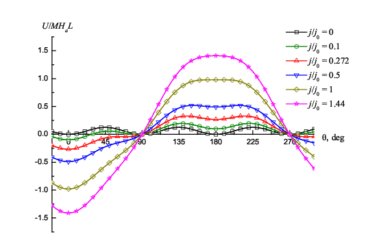
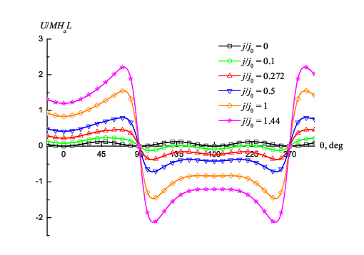
Let us present the stability analysis results for these stationary states in presence of the current under intense injection conditions (as mentioned above, the latter condition allows neglecting the STT contribution). The results are illustrated with plots of the energy as a function of the angle (Figs. 1 and 2) at various values of the current density in forward and backward directions.
1) The parallel configuration () in absence of magnetic field () is stable under forward and backward currents.
2) Under the forward current increasing from zero, the energy minimum corresponding to the original perpendicular configuration () shifts in the direction of the parallel configuration (i.e., angle decreases). This takes place up to the current density value , when the deviation from the original position reaches (i.e., ). At this value, the energy minimum disappears (it changes to an inflection point), and the system switches abruptly to a parallel configuration and remains in that configuration under further variations of the current density, so that the switching is irreversible.
Under backward current increasing from zero, the minimum corresponding to the original perpendicular configuration () shifts in the direction of the antiparallel configuration, and the corresponding angle increases up to some value that tends to
| (8) |
at the high current limit. Under returning to zero current, the perpendicular orientation restores, so that the switching by the backward current is of “temporary” character.
3) The antiparallel configuration () in a magnetic field parallel to the magnetization of the pinned layer () becomes unstable and switched to parallel one under high enough forward current. The threshold current density is
| (9) |
We see from Eq. (9) the mentioned possibility of the switching threshold lowering by means of an applied magnetic field close to (but lower than) the anisotropy field. Such an assistance of the magnetic field does not break the local character of the switching, because the magnetic field lower than the anisotropy field cannot do switching alone (without a current).
The parallel configuration appeared after switching is stable against further variations of the current, so that the switching by the forward current is irreversible.
Under the backward current, the antiparallel configuration becomes unstable at the same (in magnitude) current density , however, in this case switching takes place to a nonequilibrium stationary state or to the symmetrical state . With returning to zero current, the system does not return to antiparallel configuration, but comes to one of two perpendicular configurations or .
Thus the following variants are possible of the switching between stationary states: 1) switching an antiparallel configuration to a parallel one by turning up the forward current of density and subsequent turning off; 2) switching an antiparallel configuration to a perpendicular one by turning up the backward current of the same density and subsequent turning off; 3) switching a perpendicular configuration to a parallel one by turning up and subsequent turning off the forward current of substantially lower density .
4 Resistance of the magnetic tunnel junction
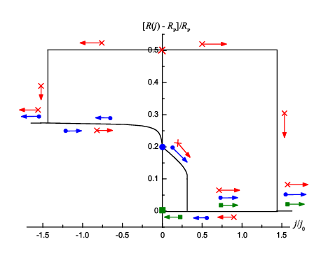
In experiments, the current-driven switching magnetic junction manifests itself, in the first place, as a change of the junction resistance. The resistance depends substantially on the relative orientation of the layers forming the junction; this is the cause of the well-known tunnel magnetoresistance effect.
The conductance of a magnetic tunnel junction with angle between the magnetization vectors of the layers takes the form [17]
| (10) |
where are the junction conductances at parallel () and antiparallel () relative orientation of the layers, respectively.
It is convenient to describe the change of the junction resistance with the following ratio:
| (11) |
where , ; is the tunnel magnetoresistance defined by usual way [18].
To find the resistance dependence on the current direction and density , it is necessary to substitute dependence to Eq. (11). With the foregoing analysis taking into account, the results are obtained shown in Fig. 3. A possibility is seen of the switching between different stationary states corresponding to different electric resistances.
5 Simulation of the magnetic junction switching dynamics
Together with the investigation of the stationary states and the switching between them, the switching dynamics is of great interest, because it determines the speed of response of the devices based on the magnetic junctions.
The time-dependent vector equation (2) describing the dynamics with using polar coordinates takes the form of a set of equations
| (12) |
| (13) |
where
| (14) |
| (15) |
The and functions describing the current effect take the form
| (16) |
| (17) |
for the forward current, and
| (18) |
| (19) |
for the backward current.
Since in fact, the precession of the free layer magnetization vector takes place in the layer plane on the whole, i.e., the vector end describes an ellipse elongated strongly in the plane. So the small terms proportional to were omitted in derivation of Eqs. (12)–(15).
In Ref. [16] an analytical solution was found of Eqs. (12), (13) at in the limiting cases of the zero damping () and strong damping (). In the general case, it is reasonable to use numerical simulation. We used the Simulink software of the MATLAB system that is intended for simulating dynamical systems [19].
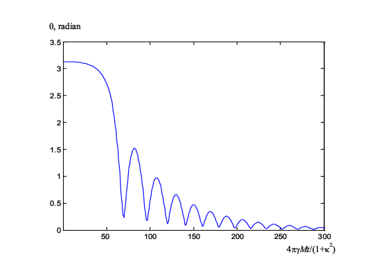
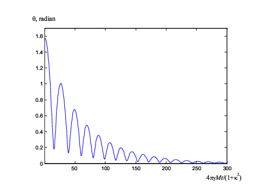
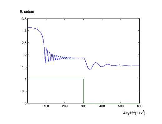
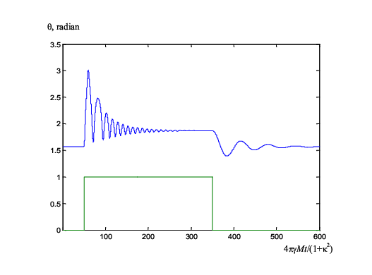
The following parameter values were given: (cf. [5]). The thermal noises initiating deviation of the free layer magnetization from the original unstable equilibrium state were imitated with giving a small initial deviation from such a state by an angle of 0.01 radians in the layer plane where the demagnetization field does not prevent fluctuation-induced deviations, so that minimal fluctuation energy is needed. The time dependences of the magnetization deviation from [100] axis under forward current of density for antiparallel and perpendicular original configuration, respectively, are shown in Figs. 4 and 5, the similar ones for the backward current are shown in Figs. 6 and 7. The dimensionless time is laid off as abscissa with as the time unit; at G one nanosecond corresponds to 200 scale divisions of the abscissa. The steps in Figs. 6 and 7 show the current turning on and turning off times.
The numerical solution (simulation) results consist completely with foregoing analysis based on the angular dependence of the magnetic energy. It is seen that direct switching occurs of the antiparallel and perpendicular configurations to parallel one under the forward current. Under the backward current, the switching occurs to an intermediate nonequilibrium stationary state, from which a transition (or return, when the initial configuration is perpendicular) occurs to the perpendicular state. As was to be expected, the switching is accompanied with damped oscillation due to precession of the magnetization vector.
With given parameter values, the characteristic switching times are of the order of nanoseconds, while the oscillation period is of the order of fractions of nanosecond. With increasing the magnetization and the damping constant, the speed of response rises (the latter up to some limits, because the switching process becomes aperiodic and slows with increasing damping at too strong damping ()).
6 Conclusion
The analysis shows a possibility of increasing the number of the switchable states by using magnetic junctions with cubic-anisotropy layers. The fact is of interest that the switching of the perpendicular configuration to the parallel one requires current density lower by several times, than the switching of the antiparallel configuration. The fruitfulness should be noted of the combination of the energy approach to determining stationary states with numerical simulation of the switching processes.
Acknowledgments
The authors are grateful to Yu. G. Kusraev, N. A. Maksimov and G. M. Mikhailov for useful discussions.
The work was supported by the Russian Foundation for Basic Research, Grant No. 08-07-00290.
References
- [1] J. Grabowski, M. Przybylski, M. Nyvlt, and J. Kirschner, J. Appl. Phys. 104, 113905 (2008).
- [2] R. Lehndorff, M. Buchmeier, D. E. Bürger D.E., et al., Phys. Rev. B 76, 214420 (2007).
- [3] S. G. Wang, R. C. C. Ward, G. X. Du, et al., Phys. Rev. B 78, 180411 (2008).
- [4] A. A. Leonov, U. K. Rößler, and A. N. Bogdanov, J. Appl. Phys. 104, 084304 (2008).
- [5] Yu. V. Gulyaev, P. E. Zilberman, A. I. Panas, and E. M. Epshtein, Zh. Eksp. Teor. Fiz. 134, 1200 (2008) [JETP 107, 1027 (2008)].
- [6] J. C. Slonczewski, J. Magn. Magn. Mater. 159, L1 (1996).
- [7] L. Berger, Phys. Rev. B 54, 9353 (1996).
- [8] C. Heide, P. E. Zilberman, and R. J. Elliott, Phys. Rev. B 63, 064424 (2001).
- [9] Yu. V. Gulyaev, P. E. Zilberman, E. M. Epshtein, and R. J. Elliott, Pis’ma Zh. Eksp. Teor. Fiz. 76, 189 (2002) [JETP Letters 76, 155 (2002)].
- [10] Yu. V. Gulyaev, P. E. Zilberman, E. M. Epshtein, and R. J. Elliott, Zh. Eksp. Teor. Fiz. 127, 1138 (2005) [JETP 100, 1005 (2005)].
- [11] R. J. Elliott, E. M. Epshtein, Yu. V. Gulyaev, and P.E. Zilberman, J. Magn. Magn. Mater. 300, 122 (2006).
- [12] Yu. V. Gulyaev, P. E. Zilberman, A. I. Krikunov, and E. M. Epshtein, Zh. Tekhn. Fiz. 77, No. 9, 67 (2007) [Techn. Phys. 52, 1169 (2007)].
- [13] E. M. Epshtein, Yu. V. Gulyaev, and P. E. Zilberman, J. Magn. Magn. Mater. 312, 200 (2007).
- [14] G. S. Krinchik, Physics of Magnetic Phenomena (Moscow State Univ. Publ., 1976) [in Russian].
- [15] R. J. Elliott, E. M. Epshtein, Yu. V. Gulyaev, and P. E. Zilberman, J. Magn. Magn. Mater. 271, 88 (2004).
- [16] E. M. Epshtein, Radiotekh. Elektron. (Moscow) 54, 339 (2009) [J. Commun. Technol. Electron. 54, 323 (2009)].
- [17] Y. Utsumi, Y. Shimizu, and H. Miyazaki, J. Phys. Soc. Japan 68, 3444 (1999).
- [18] M. Gulliere, Phys. Lett. A 54, 225 (1975).
- [19] S. T. Karris, Introduction to Simulink with Engineering Applications (Orchard Publications, 2006).