Crumpling transition of the discrete planar folding in the negative-bending-rigidity regime
Abstract
The folding of the triangular lattice embedded in two dimensions (discrete planar folding) is investigated numerically. As the bending rigidity varies, the planar folding exhibits a series of crumpling transitions at and . By means of the transfer-matrix method for the system sizes , we analyze the singularity of the transition at . As a result, we estimate the transition point and the latent heat as and , respectively. This result suggests that the singularity belongs to a weak-first-order transition.
pacs
82.45.Mp 05.50.+q 5.10.-a 46.70.HgAt sufficiently low temperatures, a polymerized membrane becomes flattened macroscopically [1]; see Refs. [2, 3, 4, 5] for a review. It still remains unclear [6, 7, 8] whether the crumpling transition (separating the flat and crumpled phases) is critical [9, 10, 11, 12, 13, 14, 15, 16, 17, 18, 19, 20, 21] or belongs to a discontinuous one with an appreciable latent heat [22, 23, 24].
In this paper, we investigate a discretized version of the polymerized membrane embedded in two dimensions [25, 26, 27, 28]; details are overviewed afterward. This model, the so-called discrete planar folding, exhibits a series of crumpling transitions at and [27, 28], as the bending rigidity changes. The latter transition exhibits a pronounced discontinuous character, whereas the nature of the former transition remains unclear. In this paper, we utilized the transfer-matrix method [27] for the system sizes . We implemented a modified folding rule [29], Eq. (5), which enables us to impose the periodic-boundary condition. Technically, the restoration of the translational symmetry admits a substantial reduction of the transfer-matrix size.
To begin with, we explain a basic feature of the discrete planar folding [27, 28]; see Fig. 1 (a). We consider a sheet of the triangular lattice. Along the edges, the sheet folds up. The fold angle is either (complete fold) or (no fold). The elastic energy at each edge is given by with the bending rigidity . The thermodynamic property of the planar folding has been studied extensively [27, 28]. The transfer-matrix simulation for the system sizes [27] revealed a series of crumpling transitions at and . The behavior of the specific heat around indicates that this transition would be a continuous one. The cluster variation method (CVM) of a single-hexagon-cluster approximation [28] indicates that there occur crumpling transitions at and of the continuous and discontinuous characters, respectively.
The crumpling transition is closely related [32] to that of an extended folding [30, 31, 32] at . (The extended folding, the so-called three-dimensional folding, has four possibilities, , as to the joint angle .) That is, according to an argument based on a truncation of the configuration space [32], the following (approximate) relations should hold;
| (1) | |||||
| (2) |
Here, the variables and denote the latent heat for the planar- and three-dimensional-folding models, respectively. A number of results, [32], [33], and [29], have been obtained via the CVM, density-matrix renormalization group, and exact-diagonalization analyses, respectively. The nature of its transition at is not fully clarified, because the three-dimensional folding is computationally demanding. It is a purpose of this paper to shed light on this longstanding issue from the viewpoint of the planar folding. (It has to be mentioned that the planar folding has to a relevance to a wide class of systems [34, 35, 36, 26, 37].)
For the sake of selfconsistency, we present the transfer-matrix formalism for the discrete planar folding explicitly. We place the Ising variables at each triangle (rather than each joint); see Fig. 1 (a). Hereafter, we consider the spin model on the dual (hexagonal) lattice. The Ising-spin configuration specifies each joint angle between the adjacent triangles. That is, provided that the spins are (anti)parallel, , for a pair of adjacent neighbors, and , the joint angle is (). The spin configuration is subjected to a constraint (folding rule); the prefactor of the transfer-matrix element, Eq. (3), enforces the constraint. As a consequence, the discrete folding reduces to an Ising model on the hexagonal lattice. In Fig. 1 (b), a drawing of the transfer-matrix strip is presented. The row-to-row statistical weight yields the transfer-matrix element. The transfer-matrix element for the strip length is given by [27]
| (3) |
with the local Hamiltonian
| (4) |
due to the bending-energy cost for spins surrounding each hexagon . Here, the parameter denotes the bending rigidity, and the expression is Kronecker’s symbol. The periodic-boundary condition is imposed. We set , considering it as a unit of energy.
In practice, the above scheme does not work. The folding rule is too restrictive to impose the periodic-boundary condition. So far, the open-boundary condition has been implemented; more specifically, the range of the running index in Eq. (3) was set to [27]. In this paper, following Ref. [29], we make a modification as to the constraint (prefactor of Eq. (3)) to surmount the difficulty. We replace the above expression with
| (5) |
That is, the constraint is released at a defect hexagon . Additionally, the local bending rigidity at the defect is set to . In order to improve the finite-size behavior, we adjust to
| (6) |
A justification is shown afterward.
Based on the transfer-matrix formalism with a modified folding rule (5), we simulated the planar folding numerically. The numerical diagonalization was performed within a subspace specified by the wave number and the parity even; here, we made use of the spin-inversion symmetry .
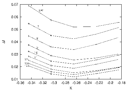
In Fig. 2, we plot the free-energy gap
| (7) |
for the bending rigidity and various system sizes . Here, the free energy per unit cell is given by with the (sub)dominant eigenvalue of the transfer matrix. [Here, the unit cell stands for a triangle of the original lattice rather than a hexagon of the dual lattice; see Fig. 1.] From Fig. 2, we see a signature of a crumpling transition (closure of ) at . The location of the transition point appears to be consistent with the preceding estimates [27, 28].
In Fig. 3, the approximate transition point is plotted for and . The approximate transition point minimizes ; namely the relation
| (8) |
holds. The least-squares fit to a series of results for yields an estimate in the thermodynamic limit . Similarly, for mod , we obtain . (An observation that the data and mod behave differently was noted in Ref. [27].) The above independent results appear to be consistent with each other, validating the -extrapolation scheme. As a result, we estimate the transition point as
| (9) |
We then proceed to estimate the amount of the latent heat with Hamer’s method [38]. A basis of this method is as follows. At the first-order transition point, the low-lying spectrum of the transfer matrix exhibits a level crossing, and the discontinuity (sudden drop) of the slope reflects a release of the latent heat. However, the finite-size artifact (level repulsion) smears out the singularity. According to Hamer [38], regarding the low-lying levels as nearly degenerate, one can resort to the perturbation theory of the degenerated case, and calculate the level splitting (discontinuity of slope) explicitly. To be specific, we consider the matrix
| (10) |
with and the transfer matrix . The bases and are the (nearly degenerate) eigenvectors of with the eigenvalues , respectively. The states are normalized so as to satisfy . According to the perturbation theory, the eigenvalues of Eq. (10) yield the level-splitting slopes due to . Hence, the latent heat (per unit cell) is given by a product of this discontinuity and the coupling constant
| (11) |
for the system size .
In Fig. 4, we plot the latent heat (11) for and . The least-squares fit for yields an estimate in the thermodynamic limit . Similarly, for mod , we obtain . Considering the deviation of these results as a possible systematic error, we obtain
| (12) |
The error margin covers both the statistical and systematic errors.
We consider the -extrapolation scheme. The finite-size data are expected to converge rapidly (exponentially) to the thermodynamic limit around the first-order transition point for periodic boundary conditions, because the correlation length (typical length scale) remains finite. Hence, the dominant finite-size corrections in our case should be described by (rather than ). On the one hand, the curve of Fig. 4 appears to be concave down, indicating an existence of a correction of O. However, this possibility (second-order phase transition) should be excluded: In a preliminary stage, we made a finite-size-scaling analysis, and arrived at a conclusion that the scaling theory does not apply; the critical index estimated from the excitation gap tends to diverge as . Therefore, we set the abscissa scale of Fig. 4 to ; actually, the result of Fig. 3 demonstrates that the abscissa scale is sensible.
As a comparison, we provide a simulation result, setting the defect parameter to tentatively. In Fig. 5, we present the free-energy gap for the bending rigidity ; the scale of is the same as that of Fig. 2, Clearly, the data of Fig. 5 are less conclusive. As a matter of fact, the signatures of the crumpling transition strongly depend on the system size . This result indicates that the choice of the defect parameter affects the finite-size behavior. In the preliminary stage, we survey a parameter space of , and arrive at a conclusion that the above choice, Eq. (6), is an optimal one.
In summary, the crumpling transition of the discrete planar folding in the regime was investigated with the transfer-matrix method for . We adopted a modified-folding rule (5), which enables us to implement the periodic-boundary condition. As a result, we estimate the transition point and the latent heat as and , respectively. The planar- and three-dimensional-folding models are closely related; see Eqs. (1) and (2). Making use of [33] and the present result , we arrive at . The relation (1) appears to hold satisfactorily; a slight deviation indicates that the truncation of the configuration space is not exactly validated. Encouraged by this result, we estimate via Eq. (2). This result is consistent with [33] and [29], indicating that the singularity belongs to a weak-first-order transition rather definitely. Because a direct approach to the three-dimensional folding is computationally demanding, an indirect information from the planar folding would be valuable. A further justification of the configuration-space truncation would be desirable to confirm this claim. This problem will be addressed in the future study.



References
- [1] D. R. Nelson and L. Peliti, J. Phys. (France) 48, 1085 (1987).
- [2] D. Nelson, T. Piran and S. Weinberg, Statistical Mechanics of Membranes and Surfaces, Volume 5 of the Jerusalem Winter School for Theoretical Physics (World Scientific, Singapore, 1989).
- [3] P. Ginsparg, F. David and J. Zinn-Justin, Fluctuating Geometries in Statistical Mechanics and Field Theory (Elsevier Science, The Netherlands, 1996).
- [4] M. J. Bowick and A. Travesset, Phys. Rep. 344, 255 (2001).
- [5] G. Gompper and D. M. Kroll, J. Phys.: Condens. Matter 9, 8795 (1997).
- [6] Y. Kantor and D. R. Nelson, Phys. Rev. Lett. 58, 2774 (1987).
- [7] Y. Kantor and D. R. Nelson, Phys. Rev. A 36, 4020 (1987).
- [8] J.-P. Kownacki and D. Mouhanna, Phys. Rev. E 79, 040101(R) (2009).
- [9] Y. Kantor, M. Kardar and D. R. Nelson, Phys. Rev. Lett. 57, 791 (1986).
- [10] Y. Kantor, M. Kardar and D. R. Nelson, Phys. Rev. A 35, 3056 (1987).
- [11] M. Baig, D. Espriu and J. Wheater, Nucl. Phys. B 314, 587 (1989).
- [12] J. Ambjørn, B. Durhuus and T. Jonsson, Nucl. Phys. B 316, 526 (1989).
- [13] R. Renken and J. Kogut, Nucl. Phys. B 342, 753 (1990).
- [14] R. Harnish and J. Wheater, Nucl. Phys. B 350, 861 (1991).
- [15] M. Baig, D. Espiu and A. Travesset, Nucl. Phys. B 426, 575 (1994).
- [16] M. Bowick, S. Catterall, M. Falcioni, G. Thorleifsson and K. Anagnostopoulos, J. Phys. I (France) 6, 1321 (1996).
- [17] J. F. Wheater and P. Stephenson, Phys. Lett. B 302, 447 (1993).
- [18] J. F. Wheater, Nucl. Phys. B 458, 671 (1996).
- [19] F. David and E. Guitter, Europhys. Lett. 5, 709 (1988).
- [20] P. Le Doussal and L. Radzihovsky, Phys. Rev. Lett. 69, 1209 (1992).
- [21] D. Espriu and A. Travesset, Nucl. Phys. B 468, 514 (1996).
- [22] M. Paczuski, M. Kardar and D. R. Nelson, Phys. Rev. Lett. 60, 2638 (1988).
- [23] J.-Ph. Kownacki and H. T. Diep, Phys. Rev. E 66, 066105 (2002).
- [24] H. Koibuchi, N. Kusano, A. Nidaira, K. Suzuki, and M. Yamada, Phys. Rev. E 69, 066139 (2004).
- [25] Y. Kantor and M. V. Jarić, Europhys. Lett. 11, 157 (1990).
- [26] P. Di Francesco and E. Guitter, Europhys. Lett. 26, 455 (1994).
- [27] P. Di Francesco and E. Guitter, Phys. Rev. E 50, 4418 (1994).
- [28] E. N. M. Cirillo, G. Gonnella and A. Pelizzola, Phys. Rev. E 53, 1479 (1996).
- [29] Y. Nishiyama, Phys. Rev. E 81, 041116 (2010).
- [30] M. Bowick, P. Di Francesco, O. Golinelli and E. Guitter, Nucl. Phys. B 450, 463 (1995).
- [31] E.N.M. Cirillo, G. Gonnella and A. Pelizzola, Phys. Rev. E 53, 3253 (1996).
- [32] M. Bowick, O. Golinelli, E. Guitter and S. Mori, Nucl. Phys. B 495, 583 (1997).
- [33] Y. Nishiyama, Phys. Rev. E 72, 036104 (2005).
- [34] J. E. Moore and D. H. Lee, Phys. Rev. B 69, 104511 (2004).
- [35] C. Castelnovo, C. Chamon, C. Mudry, and P. Pujol, Phys. Rev. B 72, 104405 (2005).
- [36] Paul Fendley, Joel E. Moore, and Cenke Xu, Phys. Rev. E 75, 051120 (2007).
- [37] R. L. Renken and J. B. Kogut, Nucl. Phys. B 350, 554 (1991).
- [38] C.J. Hamer, J. Phys. A 16, 3085 (1983).