Vicious Lévy flights

Diffusive processes with long range jumps play an important role in many physical, chemical and biological phenomena. A Lévy flight is an example of such a process where the probability distribution of the length of an individual step, $r$, is governed by the power-law $r^{-d-\sigma}$, where $d$ is the dimension of the space and $\sigma$ is the Lévy exponent. Smaller values of $\sigma$ therefore produce longer range jumps while for $\sigma\geq 2$, the mean jump length is finite and simple diffusive behavior is recovered. Lévy flights have been used to describe a wide range of processes including epidemic spreading, transcription factor proteins binding to DNA, kinetic Ising models with long-range interactions, foraging animals and light propagation in disordered optical materials [1, 2, 3, 4, 6, 5]. While individual Lévy flights have been studied in great detail, the same is not true if we consider several distinct groups of Lévy flights. One could, for example, be interested in the statistics of encounters between members of different groups. This question is relevant for processes where the outcome depends on the occurrence of such encounters. Examples include sharks and other marine animals searching for prey [7], chemical reactions in turbulent environments [8], electron-hole recombination in disordered media [9] and even male spider-monkeys encountering their mates or other aggressive males in the forest [10].

In this Letter we compute the survival probability, i.e. the probability that no two members of different groups of Lévy flights have met up to time $t$. For the case of simple diffusion with exactly one particle in each group, this corresponds to the classic problem of Gaussian vicious walks [11], i.e. walks that are prohibited from being on the same site at the same time, but remain independent otherwise. Here we generalize this concept to groups of Lévy flights under the same constraints. We term them vicious Lévy flights (VLF). We consider $p$ sets of particles with $n_{i}$ particles in each set, $i=1\dots p$, that are driven by Lévy noise on the $d$ dimensional regular lattice. A pairwise interset short-range (delta-function) interaction is introduced to guarantee that trajectories which continue beyond an intersection are discarded, i.e. have zero statistical weight. This terminates the process at the first encounter between members of different groups. Particles belonging to the same set do not interact. We note that Lévy flights are allowed to jump over each other, unlike ordinary random walks which can only jump to neighboring sites and can not intersect with the vicious constraint. In $d=1$ this means that the ordering is preserved for vicious walks but not for VLF. For simplicity we assume that Lévy exponents for all flights are the same. Generalization to the case of different Lévy exponents will be done elsewhere. At time $t=0$ all particles start in the vicinity of the origin. We are interested in the survival probability of this system at late times.

We start with a field theoretic formulation of the problem. Methods to formulate field theories for such stochastic systems are well established [12, 13]. Specifically for Gaussian vicious walks, such a formulation exists [14] and the form of the action is known. We can adapt the action to our case by replacing the Laplacian $\nabla^{2}$ with the operator $\nabla^{\sigma}$ that generates long-range jumps. This gives

where $\phi_{i}(x,t)$ are $p$ complex order parameters corresponding to $p$ different sets of equivalent Lévy flights and $\lambda_{ij}$ are coupling constants corresponding to interset interactions. The non-intersection property of VLF arises from the choice $\lambda_{ij}\to\infty$ but we will show that to leading order the survival probability does not depend on the particular value of these coupling constants. This action is also similar to the action for the reaction-diffusion problem with long-range interactions [15, 16]. Power counting shows that the upper critical dimension for the above field theory is $d_{c}=\sigma$ for $\sigma<2$ and $d_{c}=2$ for $\sigma\geq 2$. VLF exhibit different phases (see inset Figure 1) depending on the values of $d$ and $\sigma$. In the mean field phase for $d>d_{c}$ (Region I), the survival probability of VLF is non-zero at infinite time because the walks become non-recurrent and particles can avoid each other for all time. For $\sigma\geq 2$ (Region II) VLF reproduce Gaussian vicious walks. For $d<\sigma<2$ (Region III) we expect fluctuations to play an important role. In this phase, we will obtain the critical behavior of the survival probability using $\varepsilon$-expansion ($\varepsilon=\sigma-d$) around mean field theory in two-loop approximation.

We now turn to the renormalization group analysis. The propagator given by (1) is $\Gamma^{(1,1)}_{j}(s,k)=(s+k^{\sigma})^{-1}$. The particular form of the vertex in (1) leads to the fact that there are no diagrams which dress the propagator. This implies that the bare propagator is the exact propagator for the theory. The proper vertex is defined by factoring out external legs from the ordinary 4-point Green’s function of (1) $G^{(2,2)}_{ij}(s_{l},k_{l};\lambda)$. Here $\lambda=\{\lambda_{ij}\}$ is the collection of coupling constants and $(s_{l},k_{l})$ for $l=1\dots 4$ are the energy (Laplace image of time) and momenta respectively [17]. This yields

The renormalized coupling, $\lambda_{Rij}$, is the value of the proper vertex at $(s_{l}=\mu,k_{l}=0),$ for all $l$, where $\mu$ is a renormalization group flow scaling parameter. It is possible to sum all diagrams in the series with the result

where $I_{1}=(2\pi)^{-d}\int d^{d}q(2\mu+2q^{\sigma})^{-1}$. The value of the integral $I_{1}$ is given by $I_{1}=A\mu^{-\varepsilon/\sigma}\varepsilon^{-1}$, where

is the geometric factor at the leading order in $\varepsilon=\sigma-d$. By introducing the redefined coupling constant $g_{Rij}=\lambda_{Rij}\mu^{-\varepsilon/\sigma}$, we obtain the following renormalization group flow equations (see Appendix A for details):

The fixed point of this flow is $g_{*}=\varepsilon A^{-1}$. We note that this value of the fixed point is exact to all orders since all diagrams were taking into account in (3). The stability of the fixed point follows from the fact that $-\partial\beta_{ij}/\partial g_{Rij}|_{g_{Rij}=\varepsilon/A}=-\varepsilon/\sigma<0$ in the VLF region, where $\beta_{ij}=\mu\partial g_{Rij}/\partial\mu$ is renormalization group beta function.

We now consider the survival probability which is defined as the correlation function [14]

with the measure $\int{\cal D}\phi^{\dagger}{\cal D}\phi\exp[-\mathcal{S}]$. The Feynman diagram of (6) at zero order is a vertex with $2N$ external legs. Similar to the case of the $(2,2)$-vertex it is convenient to work with the truncated correlation function $\Gamma(s_{l},k_{l};\lambda)=S(s_{l},k_{l};\lambda)/\prod^{2N}_{m=1}\Gamma^{(1,1)}(s_{m},k_{m})$. The finite renormalized truncated correlation function $\Gamma_{R}(s_{l},k_{l};\lambda_{R},\mu)$, where $\lambda_{R}=\{\lambda_{Rij}\}$ is a collection of renormalized coupling constants, is related to the bare truncated correlation function by $\Gamma_{R}(s_{l},k_{l};\lambda_{R},\mu)=Z(\lambda,\mu)\Gamma(s_{l},k_{l};\lambda)$, where $Z(\lambda,\mu)$ is the scaling function. From this one obtains the renormalization group equation for $\Gamma_{R}(s_{l},k_{l};\lambda_{R},\mu)$ using the chain rule

where $\gamma=\mu\partial\ln Z/\partial\mu.$ At the fixed point (7) reduces to $(\partial/\partial\ln(\mu)+\gamma_{*})\Gamma_{R}(s,\mu)=0$ whose solution is

where $\gamma_{*}=\mu\partial\ln Z/\partial\mu|_{g_{Rij}=g_{*}}$. Since $\gamma_{*}$ is constant at the fixed point we have $\Gamma_{R}\sim\mu^{-\gamma_{*}}$. The fact that the dimensions of field and the action are $[\phi^{\dagger}]=[\phi]=k^{d/2}$ and $[\mathcal{S}]=1$ implies that $[S]=1$. Thus it follows that the survival probability can only be a function of the dimensionless product $\mu t$. From this one infers that the asymptotic behavior of the survival probability is $S(t)\sim t^{-\gamma_{*}}$ which gives $\alpha=\gamma_{*}$. In order to find $Z$ one uses a normalization condition on $\Gamma_{R}$ that fixes the value of $Z$. This can be chosen as $\Gamma_{R}(s_{l},k_{l};\lambda_{R},\mu)=1$ when $s_{l}=\mu$ and $k_{l}=0$ for all $l$. This implies that $Z=\Gamma(\mu,0;\lambda)^{-1}$. $\Gamma(\mu,0;\lambda)$ can be expressed as a series, up to two-loop order, of the integrals corresponding to the diagrams shown in Fig.2 with appropriate combinatorial factors originating from the number of distinct ways in which propagators can be assigned to the same diagram. $I_{1}$ was evaluated before. The integral corresponding to the diagram 2c is

This can be evaluated using Mellin-Barnes representation [18] which replaces the sum in the denominator of $|k+q|^{\sigma}$ and $q^{\sigma}$ by the product of these terms raised to some power. The result for $I_{2}$ up to the leading order reads

where $C=[\psi^{(0)}(\sigma/2)+\log(4\pi)]/2$ and $\psi^{(0)}(x)$ is standard digamma function. The details of the calculations are summarized in Appendix B. Knowing $I_{1},I_{2}$ and the appropriate combinatorial factors allows us to evaluate $\Gamma(\mu,0;\lambda)$ and therefore $Z(\mu,\lambda)$ as a series. Differentiating $\ln Z$ with respect to $\mu$ and substituting $\lambda$ with $\lambda_{R}$ (inverting (3)) and then taking the value at the fixed point gives us the survival probability exponent $\alpha=\gamma_{*}$, with the final result (see Appendix C):

where $Q=6\sum_{1\leq i<j<k\leq p}n_{i}n_{j}n_{k}+\sum_{1\leq i<j\leq p}n_{i}n_{j}(n_{i}+n_{j}-2)$. At the critical dimension $d=d_{c}=\sigma$ we see that the fixed point coincides with the Gaussian point. The interaction becomes marginal in the renormalization group sense. Equation (5) then yields the flow equations for the running coupling constant

with initial condition $\bar{g}_{ij}(1)=g_{Rij}.$ Solving this and substituting the result into (8) we get $S(t)=(\ln t)^{-\alpha_{l}},$ where

Now we describe the details of the numerical simulation that we used to confirm our results in $d=1$. At $t=0$ we start with $N=\sum_{i=1}^{p}n_{i}$ particles belonging to $p$ distinct sets placed equidistantly on the lattice. At each time step we generate $N$ random variables, $x_{j}$, drawn from the uniform distribution on the interval $(0,1)$. Each particle jumps a distance $l_{j}=x_{j}^{-1/\sigma}$ with equal probability to the left or to the right. This procedure generates an independent Lévy flight trajectory for each particle. The process stops whenever particles from different sets land on the same site. We perform $\sim 10^{5}$ iterations for each set of parameter values. The survival probability $S(t)$ is defined by the number of processes that survived beyond time $t$ divided by the total number of iterations. Figure 1 shows the plot of the survival probability as a function of time for $N=2$ for different values of $\sigma$. It is clear that at late times $\ln S(t)$ is linear in $\ln t$ verifying our predicted power-law decay $S(t)\sim t^{-\alpha}$. The critical exponent $\alpha$ is evaluated from the slope of the best fit line of the late time data.

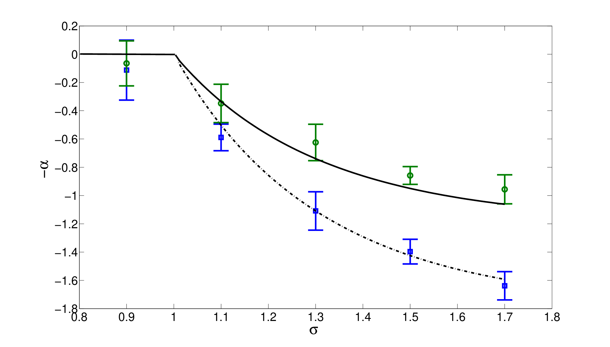
We first consider systems with exactly one particle in each set. Figure 3 shows the value of exponent $\alpha$ for various values of $\sigma$ with the total number of particles $N=2,3$ and $4$ in $d=1$. Values of $\sigma\geq 2$ will reproduce Gaussian vicious walks and we therefore expect our exponents to approach the exact Fisher exponents [11] as seen in Figure 3. For two VLF higher loop corrections are absent (see (11)) and the one-loop result is an exact result in agreement with the simulation. It is interesting to note that the survival probability for the $N=2$ case is equivalent to the first return probability of a single Lévy flight to the origin after time $t$ which scales as $t^{-1+d/\sigma}$ [19] and matches our results. For $\sigma<1$, or $d>d_{c}$, we expect mean field behavior where survival probability at late times approaches a non-zero value implying that there is a finite probability that Lévy flights with $\sigma<1$ will never find each other. The fact that the survival probability tends to a constant at late times is reflected in the small values of $\alpha$ for $\sigma=0.9$. For $1<\sigma<2$, the mean field behavior is incorrect and we expect the fluctuations to shift the decay exponent to some non-trivial value. For $\sigma$ close to one, the 1-loop result is in good agreement with the simulation. For larger values of $\sigma$, the 2-loop corrections perform better (see Fig.3 inset). It is to be noted that the discrepancy between theory and simulation becomes large for higher values of $N$ because the combinatorial factors in (11) become large and we therefore need to keep higher order terms in $\varepsilon$ for the same degree of accuracy. It is interesting that the 1-loop approximation works reasonably well over the entire range of $1<\sigma\leq 2$ simply because the 1-loop term in (11) happens to give the exact Fisher result if we set $\sigma=2$. We notice that in all cases the value of the survival probability exponent $\alpha$ increases with $\sigma$ starting from $\alpha\sim 0$ at $\sigma<1$ and rising to the value of the Fisher exponents for the equivalent Gaussian vicious walks. This is in contrast to diffusion-annihilation reactions with long-range jumps where the density of reactants decays faster for smaller values of $\sigma$ [16].

We now consider a system that consists of 2 sets of identical VLF with different numbers of independent particles in each set. We shall call one set predators and the other set prey. Figure 4 compares the values of the 2-loop exponents to the simulation results for various values of $\sigma$ for two different cases: 4 predators - 1 prey and 3 predators - 2 prey. Similar to the previous case we have mean field and Gaussian behaviors for $\sigma<1$ and $\sigma\geq 2$ respectively. The Gaussian case is also known as the lion-lamb problem and has been studied before [20]. Unlike the lion-lamb problem, however, our results do not depend on the initial ordering of predators and prey because ordering is not preserved for VLF. For a given $\sigma$ and total number of predators plus prey, the number of potentially lethal encounters is maximized when the difference between the number of predators and prey is the smallest implying that the survival probability will decay faster as seen in Fig.4.

Our results suggest that it is interesting to solve the problem in the general case of particles with different diffusion constants and Lévy exponents. The predictive power of the $\varepsilon$-expansion for VLF, that we have demonstrated, should be useful in many applications of practical importance. Examples include the optimization of the predator-prey search [21] or trapping probabilities [22]. Generalization to the case of intelligent predators, i.e. interacting with a prey by means of the long-range potential, may lead to different critical behavior [23, 24, 25]. Simple diffusion processes in power-law small world networks are effectively Lévy flights [26] with the exponent $\sigma$ controlling the distribution of long-range links. Our work could be used to understand what network structure, or what $\sigma$, would optimize the search and how much more efficient several independent searchers will be.

The authors would like to acknowledge UC Merced start-up funds and a James S. McDonnell Foundation Award for Studying Complex Systems.

References

- [1] R. Metzler and J. Klafter, Phys. Rep. 339, 1 (2000).
- [2] M. A. Lomholt, B. van den Broek, S.-M. J. Kalisch, G. J. L. Wuite and R. Metzler, PNAS 106, 8204 (2009).
- [3] N. Menyhard and G. Odor J. Phys. A: Math. Gen. 28, 4505 (1995).
- [4] B. Bergersen and Z. Rácz, Phys. Rev. Lett. 67, 3047 (1991).
- [5] P. Barthelemy, J. Bertolotti and D. S. Wiersma, Nature 453, 495 (2008).
- [6] G. M. Viswanathan, V. Afanasyev, S. V. Buldyrev, E. J. Murphy, P. A. Prince and H. E. Stanley Nature 381, 413 (1996).
- [7] D. W. Sims et al, Nature 451, 1098 (2008).
- [8] M. F. Shlesinger, B. J. West and J. Klafter, Phys. Rev. Lett. 58, 1100 (1987).
- [9] M. F. Shlesinger, Nature 411, 641 (2001).
- [10] G. Ramos-Fernandez, J. L. Mateos, O. Miramontes, G. Cocho, H. Larralde and B. Ayala-Orozco, Behav. Ecol. Sociobiol. 55, 223 (2004).
- [11] M. E. Fisher, J. Stat. Phys. 34, 667 (1984).
- [12] M. Doi, J. Phys. A: Math. Gen. 9, 1465 (1976).
- [13] L. Peliti, J. Physique 46, 1469 (1985).
- [14] J. Cardy and M. Katori, J. Phys. A 36, 609 (2003).
- [15] H. K. Janssen and O. Stenull, Phys. Rev. E 78, 061117 (2008).
- [16] H. Hinrichsen, J. Stat. Mech.: Theor. Exp. P07066 (2007).
- [17] J. B. Bronzan and J. W. Dash, Phys. Rev. D 10, 4208 (1974).
- [18] V. A. Smirnov, Evaluating Feynman Integrals, (Springer, 2004).
- [19] R. Metzler and J. Klafter, J. Phys. A 37, R161 (2004).
- [20] S. Redner, P. L. Krapivsky, Am. J. Phys. 67, 1277 (1999).
- [21] F. Bartumeus, J. Catalan, U. L. Fulco, M. L. Lyra, and G. M. Viswanathan, Phys. Rev. Lett. 88, 097901 (2002).
- [22] R. F. Kayser and J. B. Hubbard Phys. Rev. Lett. 51, 79 (1983)
- [23] I. Goncharenko and A. Gopinathan; arXiv:1003.5970.
- [24] G. Schehr, S. N. Majumdar, A. Comtet and J. Randon-Furling, Phys. Rev. Lett. 101, 150601 (2008).
- [25] C. Nadal and S. N. Majumdar, Phys. Rev. E 79, 061117 (2009).
- [26] B. Kozma, M. B. Hastings and G. Korniss, Phys. Rev. Lett. 95, 018701 (2005).
- [27] I. S. Gradshtein I. M. Ryjik Tables of Integrals, (Academic Press, 1965).