$K\pi$ vector form factor constrained by $\tau\to K\pi\nu_{\tau}$ and $K_{l_{3}}$ decays

The differential decay distributions of $K\to\pi\,l\,\nu_{l}$ ($K_{l_{3}}$) and $\tau\to K\pi\nu_{\tau}$ decays are governed by two Lorentz-invariant $K\pi$ form factors that encode the non-perturbative physics, namely the vector, denoted $F^{K\pi}_{+}(q^{2})$, and the scalar, $F^{K\pi}_{0}(q^{2})$. According to the kinematical configuration, $q$ represents the exchanged ($K_{l_{3}}$) or the total ($\tau\to K\pi\nu_{\tau}$) $K\pi$ four-momentum. A good knowledge of these form factors is of fundamental importance for the determination of many parameters of the Standard Model, such as the quark-mixing matrix element $|V_{us}|$ obtained from $K_{l_{3}}$ decays [1], or the strange-quark mass $m_{s}$ determined from the scalar QCD strange spectral function [2]. Recently, several collaborations have produced data for $K_{l_{3}}$ decays and new high-statistics data for $\tau\to K\pi\nu_{\tau}$ have been published by the $B$ factories. The new data sets provide the substrate for up-to-date theoretical analyses of the $K\pi$ form factors.

Historically, the main source of experimental information on $K\pi$ form factors have been $K_{l_{3}}$ decays. Recently, five experiments have collected data on semileptonic and leptonic $K$ decays: BNL-E865 [3], KLOE [4], KTeV [5], ISTRA+ [6], and NA48 [7]. The results from these analyses yielded an important amount of information on form factors as well as stringent tests of QCD at low-energies and of the Standard Model itself (for recent reviews on theoretical and experimental aspects of kaon physics we refer to Refs. [8, 9]). Additional knowledge on the $K\pi$ form factors can be gained from the dominant Cabibbo-suppressed $\tau$ decay: the channel $\tau\to K\pi\nu_{\tau}$. The $\tau$ is the only known lepton heavy enough to decay into hadrons and its hadronic decays constitute a rather clean environment for the study of QCD at relatively low energies [10] and notably for the determination of the QCD coupling $\alpha_{s}$ [11, 12, 13, 14]. In the 1990s, the $K\pi$ spectrum for $\tau\to K\pi\nu_{\tau}$ was measured by ALEPH [15] and OPAL [16]. Lately, however, the $B$ factories have become a superior source of high-statistics data for this reaction by virtue of the important cross-section for $e^{+}e^{-}\to\tau^{+}\tau^{-}$ around the $\Upsilon(4S)$ peak. As a result, as many as $10^{9}$ $\tau$ pairs were recorded by Belle and BaBar [17]. A detailed spectrum for $\tau\to K_{S}\,\pi^{-}\nu_{\tau}$ produced and analysed by Belle was published in 2008 [18] with an event sample larger than in the LEP experiments by almost a factor of 65, allowing for a detailed analysis of its shape. Also, a preliminary BaBar spectrum with similar statistics has appeared recently in conference proceedings [19] and, finally, BESIII should produce results for this decay in the future [20].

On the theory side, a salient feature of the form factors in the kinematical region relevant for $K_{l_{3}}$ decays, i.e. $m_{l}^{2}<q^{2}<(m_{K}-m_{\pi})^{2}$, is that they are real. Within the allowed phase-space they admit a Taylor expansion and the energy dependence is customarily translated into constants $\lambda_{+,0}^{(n)}$ defined as¹¹ 1 From now on we refrain from writing the superscript $K\pi$ on the form factors.

In $\tau\to K\pi\nu_{\tau}$ decays, however, since $(m_{K}+m_{\pi})^{2}<q^{2}<m_{\tau}^{2}$, one deals with a different kinematical regime in which the form factors develop imaginary parts, rendering the expansion of Eq. (1) inadmissible. One must then resort to more sophisticated treatments. Moreover, in order to fully benefit from the available experimental data, it is desirable to employ representations of the form factors that are valid for both $K_{l_{3}}$ and $\tau\to K\pi\nu_{\tau}$ decays. In Ref. [21], a new expression for $F_{+}(s)$ was derived within the Resonance Chiral Theory (RChT) framework [22] and, subsequently, the authors reanalysed the Belle spectrum for the decay $\tau\to K\pi\nu_{\tau}$ with success [23]. This analysis yielded new values for the constants $\lambda_{+}^{\prime}$ and $\lambda_{+}^{\prime\prime}$ emphasising the interplay between $\tau\to K\pi\nu_{\tau}$ and $K_{l_{3}}$ experiments.

From general principles of analyticity, the form factors must fulfil a dispersion relation. Unitarity provides an additional constraint on the imaginary part of the form factors, rendering possible the design of dispersive representations of $F_{+}$ and $F_{0}$ that are suited to describe both $\tau\to K\pi\nu_{\tau}$ and $K_{l_{3}}$ decays. For the vector form factor, a step towards this feat was taken in Refs. [24, 25] where we introduced several subtracted dispersive representations of $F_{+}$. Our final proposal was a three-times-subtracted dispersive representation in which $\lambda_{+}^{\prime}$ and $\lambda_{+}^{\prime\prime}$ are parameters that were determined via a successful fit to the Belle spectrum. A similar dispersive approach to $F_{+}$ was presented in Ref. [26] and has been used by the KTeV collaboration to fit their $K_{l_{3}}$ spectra [27]. Finally, a dispersive representation for $F_{+}$ that includes inelastic effects was introduced in Ref. [28]. Concerning the scalar form factor, a thorough description that takes into account analyticity, unitarity, the large-$N_{c}$ limit of QCD, and the coupling to $K\eta$ and $K\eta^{\prime}$ channels was introduced in Ref. [29] and updated in Refs. [2, 30, 31]. Another single-channel dispersive representation of $F_{0}$ can be found in Ref. [32] and a description based on the so-called method of unitarity bounds was recently presented in Ref. [33].

The main purpose of our paper is to produce an analysis of the Belle spectrum for $\tau\to K\pi\nu_{\tau}$ incorporating constraints from experimental results on $K_{l_{3}}$ decays. We have already advocated that such a combined treatment of both reactions could further our knowledge of the form factors hence paving the way for a better determination of $|V_{us}|$ [25]. Moreover, we aim at extracting as much information as possible from the $\tau\to K\pi\nu_{\tau}$ spectrum. With the present statistics the spectrum allows for a study of $K\pi$ dynamics in the $P$ wave, which gives the prevailing contribution to the decay. Watson’s theorem [34] guarantees that below inelastic thresholds the phase of the form factor equals the scattering phase and, therefore, one can perform a study of the dominant $K\pi$ $P$-wave threshold parameters. In addition, it has been shown [23, 24] that the present statistics permits a competitive determination of the pole position of the $K^{*}(892)^{\pm}$ as well as the position of a second vector resonance, although less precisely in the latter case. Here, we determine these two poles exploiting a novel strategy in which fits are done directly in terms of the physical pole positions on the second Riemann sheet. This improvement with respect to previous works [18, 23, 24] yields a determination of the pole positions with a better control of uncertainties and correlations.

In our analysis, for the vector form factor we employ the dispersive representation of Ref. [24] whereas for the scalar $K\pi$ form factor we use the up-to-date results of Ref. [31]. Since the details of these descriptions can be found in the original works, here we shall concentrate on the results that arise from our fit, namely i) the pole positions for the $K^{*}(892)^{\pm}$ and $K^{*}(1410)^{\pm}$ resonances, ii) $\lambda_{+}^{\prime}$ and $\lambda_{+}^{\prime\prime}$, iii) the result of the phase-space integrals needed in $K_{l_{3}}$ decays, and iv) the $K\pi$ isospin-$1/2$ $P$-wave scattering phase and the respective threshold parameters.

Our paper is organised as follows. First, in Sec. 2, we briefly review the dispersive treatment of the vector and scalar $K\pi$ form factors. Then, in Sec. 3, we present a fit to $\tau\to K\pi\nu_{\tau}$ data alone. In Sec. 4, the results for a fit incorporating constraints from $K_{l_{3}}$ experiments are given and, in Sec. 5, we derive our results for the phase-space integrals relevant for $K_{l_{3}}$ experiments. We discuss the results for the $K\pi$ threshold parameters and scattering phase shifts in Sec. 6. Our final results and a comparison with other results found in the literature are presented in Sec. 7.

The $K\pi$ form factors are defined as follows [8]

where $F_{+}(q^{2})$ and $F_{0}(q^{2})$ are the vector and scalar form factors respectively and $q^{2}=(k-p)^{2}$. It follows from the definition that both form factors share the same normalisation at zero $F_{+}(0)=F_{0}(0)$. For convenience, we work with normalised form factors $\tilde{F}_{+,0}(q^{2})$ such that

First, in determinations of $|V_{us}|$, a reliable value for the normalisation at zero is crucial in order to disentangle the product $|V_{us}|F_{+}(0)$. In this respect, Chiral Perturbation Theory (ChPT) and lattice QCD are the most trustworthy methods to obtain $F_{+}(0)$. Here we are concerned with another aspect of the form factors, namely their energy dependence encoded in $\tilde{F}_{+,0}(q^{2})$. The precise knowledge of $\tilde{F}_{+,0}(q^{2})$ is needed when performing the phase space integrals for $K_{l_{3}}$ decays or when studying in detail the $\tau\to K\pi\nu_{\tau}$ spectrum. Finally, one should bear in mind that when considering $\tau$ decays, one deals with a crossing-symmetric version of Eq. (2) for the $K\pi$ pair is in the final state. In this case, $q^{2}\equiv s=(k+p)^{2}>(m_{K}+m_{\pi})^{2}$ and the form factors develop imaginary parts.

In $\tau\to K\pi\nu_{\tau}$ and $K_{e_{3}}$ decays, the term containing the vector form factor $F_{+}(q^{2})$ dominates the differential decay widths. The form factor, in its turn, receives a prevailing contribution from the $K^{*}(892)$. This fact motivated the description of Refs. [21, 23] within RChT, which was based on an analogous treatment of the pion vector form factor [37, 38]. Although dominated by the $K^{*}(892)$, the authors of Refs. [21, 23] noted that a second resonance, identified with the $K^{*}(1410)$, must be included in $F_{+}(s)$ to account for the higher-energy part of the $\tau\to K\pi\nu_{\tau}$ spectrum. The description of Refs. [21, 23], albeit successful, has a slight drawback, namely it satisfies the analyticity constraints only in a perturbative sense. Although the violation of analyticity is expected to be of higher orders in the chiral expansion, a description based on a dispersive treatment was necessary to corroborate this pattern. In Ref. [24] we designed such dispersive representations of $F_{+}(s)$.

The rationale for our approach is as follows. From general principles, the form factor must satisfy a dispersion relation. Supplementing this constraint with unitarity, the dispersion relation has a well-known closed-form solution within the elastic approximation referred to as the Omnès representation [39]. Although simple, this solution requires the detailed knowledge of the phase of $F_{+}(s)$ up to infinity, which is unrealistic. An advantageous strategy to circumvent this problem is the use of additional subtractions, as done for the pion form factor in Ref. [40]. Subtractions in the dispersion relation entail a suppression of the integrand in the dispersion integral for higher energies. An $n$-times-subtracted form factor exhibits a suppression of $s^{-(n+1)}$ in the integrand. Thereby, the information that was previously contained in the high-energy part of the integral is translated into $n-1$ subtraction constants. In Ref. [24] we performed fits to the Belle spectrum of $\tau\to K\pi\nu_{\tau}$ varying the number of subtractions and testing the description with one and two vector resonances. The outcome of these tests, described in detail in Ref. [24], is that for our purposes an optimal description of $F_{+}(s)$ was reached with three subtractions and two resonances. Here we quote the resulting expression

In the last equation, $s_{K\pi}=(m_{K^{0}}+m_{\pi^{-}})^{2}$ and the two subtraction constants $\alpha_{1}$ and $\alpha_{2}$ are related to the Taylor expansion of Eq. (1) as $\lambda_{+}^{\prime}=\alpha_{1}$ and $\lambda_{+}^{\prime\prime}=\alpha_{2}+\alpha_{1}^{2}$. It is opportune to treat them as free parameters that capture our ignorance of the higher energy part of the integral. The constants $\lambda_{+}^{\prime}$ and $\lambda_{+}^{\prime\prime}$ can then be determined through the fit. The main advantage of this procedure, advocated for example in Refs. [40, 32, 26, 24], is that the subtraction constants turn out to be less model dependent as they are determined by the best fit to the data. The calculation of these constants, on the other hand, depends strongly on the perfect knowledge of $\delta(s)$. However, since now $\alpha_{1,2}$ are determined by the data, in the limit $s\to\infty$ the asymptotic behaviour of $F_{+}(s)$ cannot be satisfied. This is so because a perfect cancellation between terms containing $\alpha_{1}$ and $\alpha_{2}$ with polynomial terms coming from the dispersion integral must occur in order to guarantee that $F_{+}(s)$ vanishes as $1/s$. We have checked that our form factor, within the entire range where we apply it (and beyond), is indeed a decreasing function of $s$ which renders this approach credible.

With Eq. (4), the transition from the kinematical region of $\tau\to K\pi\nu_{\tau}$ to that of $K_{l_{3}}$ decays is straightforward and the dominant low-energy behaviour of $F_{+}(s)$ is encoded in $\lambda_{+}^{\prime}$ and $\lambda_{+}^{\prime\prime}$. The cut-off $s_{\rm cut}$ in the dispersion integral is introduced to quantify the suppression of the higher energy part of the integrand. The stability of the results is checked varying this cut-off in a wide range from $1.8\,\mbox{GeV}<\sqrt{s_{\rm cut}}<\infty$. It is important to stress that Eq. (4) remains valid beyond the elastic approximation provided $\delta(s)$ is the phase of the form factor, instead of the corresponding scattering phase. But, of course, in order to employ it in practice we must have a model for the phase. As described in detail in Ref. [24], we take a form inspired by the RChT treatment of Refs. [21, 23] with two vector resonances. Here we relegate the details concerning $\delta$ to Appendix A. However, one important remark is in order. Since we keep the real part of the loop bubble integral $\mbox{Re}\,\tilde{H}(s)$ in Eq. (26), the mass and width parameters of Ref. [24] are shifted as compared with those of Refs. [18, 21, 23]. This shift emphasises the need for the computation of the physical pole position of the resonances on the second Riemann sheet. We have shown [24, 25] that although the mass and width parameters from Refs. [18, 23, 24] differ considerably, the pole positions arising from the models are in good agreement. To clarify this issue further, in this work we implement a numerical improvement in our codes that allows us to perform the fits directly in terms of the pole positions on the second Riemann sheet. This new procedure is clearer as it avoids the cumbersome intermediate stage where one must compute the pole positions from the unphysical parameters to obtain meaningful results [36]. Furthermore, correlations and uncertainties are obtained directly for the physical poles and are therefore more reliable.

In the previous analysis of Refs. [23, 24] the scalar form factor was shown to play an important role for the low-energy part of the $\tau\to K\pi\nu_{\tau}$ spectrum, between threshold and $\sim 0.8$ GeV. On the other hand, the fit was not very sensitive to the details of $F_{0}$ as it is in the case of $F_{+}$. Therefore, we again rely on the coupled channel representation of $F_{0}$ first presented in Ref. [29] and updated in Refs. [2, 30, 31]. The main features of this treatment can be found in Appendix A.

Before proceeding to a fit that combines information from $\tau\to K\pi\nu_{\tau}$ and $K_{l_{3}}$ data, we shall perform in this section a short update of Ref. [24]. The aim is twofold. First we want to ascertain the impact of performing the fit directly in terms of the physical pole positions for the vector resonances. Second, the results of this section serve as a point of reference for the new analysis. For the sake of completeness, we recall here how the $K\pi$ form factors enter the description of $\tau\to K\pi\nu_{\tau}$.

Assuming isospin invariance, the differential decay distribution for $\tau\to K\pi\nu_{\tau}$ can be cast in terms of the $K\pi$ form factors as

where we summed over the two possible decay channels $\tau^{-}\to\bar{K}^{0}\pi^{-}\nu_{\tau}$ and $\tau^{-}\to K^{-}\pi^{0}\nu_{\tau}$ that contribute in the ratio $2:1$. In Eq. (5), $S_{\mbox{\tiny EW}}$ is an electroweak correction factor, $\Delta_{K\pi}\equiv m_{K}^{2}-m_{\pi}^{2}$, $s=(k+p)^{2}$ with $k$ and $p$ being respectively the kaon and pion momenta, and

is the kaon momentum in the rest frame of the hadronic system. In order to analyse the data, one must rely on an ansatz for the number of events observed in a given bin of the experimental spectrum. As explained in Ref. [23] the theoretical number of events $N_{i}^{\rm th}$ in the $i$-th bin is taken to be

where $\mathcal{N}_{T}$ is the total number of events, the factor $\frac{1}{2}$ and $\frac{2}{3}$ account for the fact that the $K_{S}\pi^{-}$ channel was analysed, $\Delta^{i}_{\rm b}$ is the width of the $i$-th bin, $\Gamma_{\tau}$ is the total $\tau$ decay width, $\bar{B}_{K\pi}$ is a normalisation constant that, for a perfect description of the spectrum, should be the $\tau\to K\pi\nu_{\tau}$ branching ratio, and, finally, $s_{\rm b}^{i}$ is the centre of the $i$-th bin. In the case of Belle’s spectrum [18] one has $\mathcal{N}_{T}=53110$ and a constant bin width $\Delta_{\rm b}=11.5$ MeV.

In this fit, we minimise the $\chi^{2}$ function given by

where $N^{\rm exp}_{i}$ and $\sigma_{N^{\rm exp}_{i}}$ are, respectively, the experimental number of events and the corresponding uncertainty in the $i$-th bin. The prime in the symbol of sum indicates that bins 5, 6, and 7 are excluded from the minimisation²² 2 If these three points are included in the fit the results do not change significantly although the $\chi^{2}$ is larger. Furthermore, there is no indication for a peak at this energy and BaBar spectra do not display a bump close to threshold. Hence, we decided, following Refs. [23, 24], to exclude these points. For a visual account, points not included in the $\chi^{2}$ are shown as unfilled circles in Fig. 1.. In the $\chi^{2}$, following a suggestion of the experimentalists [35], we include data up to bin number 90 which corresponds to $\sqrt{s}=1.65925$ GeV. Finally, the lowest data point is not taken into account since, with physical meson masses, its centre lies below the $K\pi$ threshold. The second term on the right-hand side of Eq. (8) was not included in the $\chi^{2}$ function of Ref. [24]. It introduces an additional restriction that allows us to treat the normalisation $\bar{B}_{K\pi}$ of Eq. (7) as a free parameter. Then, the parameters of the fit are 8 in total. First, the two constants $\lambda_{+}^{\prime}$ and $\lambda_{+}^{\prime\prime}$ responsible for the behaviour of $\tilde{F}_{+}(s)$ near the origin. Second, the five parameters that determine the resonance properties, i.e. the complex pole positions of the $K^{*}(892)$ and³³ 3 For simplicity, in tables we refer to the $K^{*}(892)$ and the $K^{*}(1410)$ simply as $K^{*}$ and $K^{*\prime}$ respectively. $K^{*}(1410)$ and the mixing parameter $\gamma$ [see Eq. (25)]. The mass and width of the resonances are extracted from the complex pole position $s_{R}$ as [36]

The phase of the form factor is fully determined by the latter set of parameters. The 8th parameter of the fit is the normalisation $\bar{B}_{K\pi}$.

In the fit, we employ the following numerical values: $|V_{us}|F_{+}(0)=0.2163(5)$ [9], $G_{F}=1.16637(1)\times 10^{-5}$ GeV^-2 [41], $m_{\tau}=1776.84$ MeV [41], $S_{\rm EW}=1.0201(3)$ [42], $f_{\pi}=92.21(14)$ MeV [43], $f_{K}/f_{\pi}=1.197(6)$ [43], and $B^{\rm exp}_{K\pi}=0.418(11)\%$ [44, 45]. We recall that the cut-off $s_{\rm cut}$ of Eq. (4) has to be varied in order to check the stability of the results upon the high-energy part of the dispersion integral. When quoting final results one must therefore include an uncertainty due to the small residual dependence on $s_{\rm cut}$. The results of fits with four values of $s_{\rm cut}$, namely $s_{\rm cut}=3.24$ GeV², 4 GeV², 9 GeV², and $s_{\rm cut}\to\infty$, are displayed in Tab. 1.

Some of the results of Tab. 1 are to be compared with those of Tab. 4.2 of Ref. [24]. Concerning $\lambda_{+}^{\prime}$, $\lambda_{+}^{\prime\prime}$ and $\gamma$ they are very similar if not identical. However, in Ref. [24], the $\chi^{2}$ that was minimised did not include the second term in the right-hand side of Eq. (8) and therefore $\bar{B}_{K\pi}$ was kept fixed or, otherwise, the strong positive correlation between $\bar{B}_{K\pi}$ and the constant $\lambda_{+}^{\prime}$ would render a good determination of these parameters impracticable. The main difference between the two fits lies, as already stressed, in the pole positions of the vector resonances. In Tab. 1, the results correspond to physical masses and widths obtained from the pole positions in the second Riemann sheet according to Eq. (9) whereas the results of Tab. 4.2 of Ref. [24] are non-physical parameters. Consequently, results for masses and widths presented here should not be directly compared with the parameters of Tab. 4.2 of Ref. [24]. Instead, one should compare with the physical poles that can be found in Eqs. (5.4) and (5.5) of Ref. [24]. One sees that the central values agree nicely. On the other hand, the treatment of the uncertainties affecting the poles is here much more trustworthy. The results of Tab. 1 come from an analysis performed by the MINOS function of the CERN-Minuit library. The errors are smaller than the ones quoted in Ref. [24] due to the proper inclusion of correlations. Finally, the fit is very stable against changes in $s_{\rm cut}$. This is specially true for the mass and width of the $K^{*}(892)$ but in all other cases variations are at most at the level of one standard deviation. In order to produce a feeling for the correlation coefficients between the parameters of our fits, as an example we display in Tab. 2 those corresponding to $s_{\rm cut}=4$ GeV².

Dispersive representations of $K\pi$ form factors can be used in order to simultaneously fit both $\tau\to K\pi\nu_{\tau}$ and $K_{l_{3}}$ spectra. We have recently advocated [25], performing Monte Carlo (MC) simulations, that the main benefit of such a combined fit would be the reduction of the uncertainties on the parameters $\lambda_{+}^{\prime}$ and $\lambda_{+}^{\prime\prime}$, leading to smaller uncertainties in the phase-space integrals needed for the extraction of $V_{us}$ from kaon decays. For the want of an unfolded data set from $K_{l_{3}}$ experiments, we perform here a fit to $\tau\to K\pi\nu_{\tau}$ constrained by results for $\lambda_{+}^{\prime}$ and $\lambda_{+}^{\prime\prime}$ obtained from a compilation of $K_{l_{3}}$ analyses [9].

In results obtained from quadratic representations such as the one of Eq. (1), the errors on $\lambda_{+,0}^{(n)}$ have a clear statistical meaning. In principle, therefore, it is straightforward to include that information in the $\chi^{2}$ that is to be minimised by the fit. In this case, the statistical correlation between $\lambda_{+}^{\prime}$ and $\lambda_{+}^{\prime\prime}$ must be taken into account. The $\chi^{2}$ to be minimised contains then one additional term

where the first two terms in the right-hand side are the same as in Eq. (8) whereas the last one encodes the information from $K_{l_{3}}$ analyses. In this last term, the vectors $\mbox{\boldmath$\lambda$}_{+}^{\rm th,exp}$ are given by

and the $2\times 2$ matrix $V$ is the experimental error matrix for $\mbox{\boldmath$\lambda$}_{+}$ such that

where the indices refer to $\lambda_{+}^{\prime}$ and $\lambda_{+}^{\prime\prime}$, $\rho_{ij}$ is the correlation coefficient ($\rho_{ij}=1$ if $i=j$), and $\sigma_{i}$ the experimental errors on $\lambda_{+}^{\prime}$ and $\lambda_{+}^{\prime\prime}$. For the experimental values we employ the results of the compilation of $K_{L}$ analyses performed by Antonelli et al. for the FlaviaNet Working Group on Kaon Decays in Ref. [9]: $\lambda_{+}^{\prime\,\rm exp}=(24.9\pm 1.1)\times 10^{-3}$, $\lambda_{+}^{\prime\prime\,\rm exp}=(16\pm 5)\times 10^{-4}$ and $\rho_{\lambda_{+}^{\prime},\lambda_{+}^{\prime\prime}}=-0.95$. Results for fits using the $\chi^{2}$ function of Eq. (10) with $s_{\rm cut}=3.24$ GeV², 4 GeV², 9 GeV², and $s_{\rm cut}\to\infty$ are shown in Tab. 3. In Fig. 1, the Belle spectrum for $\tau\to K\pi\nu_{\tau}$ is confronted with the results for the fit with $s_{\rm cut}=4$ GeV². Finally, as an example, the correlation matrix for $s_{\rm cut}=4$ GeV² is given in Tab. 4.

Comparing the results of the fit constrained by $K_{l_{3}}$ analyses, Tab. 3, with the results of the fit to $\tau\to K\pi\nu_{\tau}$ alone, Tab. 1, one sees that the statistical uncertainty in $\lambda_{+}^{\prime}$ and $\lambda_{+}^{\prime\prime}$ is reduced roughly by a factor of 2. Another advantage of the new fit is that the results for $\lambda_{+}^{\prime}$ and $\lambda_{+}^{\prime\prime}$ are much more stable against changes in $s_{\rm cut}$. The errors in $\lambda_{+}^{\prime}$ are largely dominated by statistics in sharp contrast with Tab. 1 where the model dependent uncertainties arising from the $s_{\rm cut}$ dependence were of the same order as the statistical ones. The central results of $\lambda_{+}^{\prime}$ and $\lambda_{+}^{\prime\prime}$ exhibit a small shift because $K_{l_{3}}$ experiments favour larger values. The mass of the $K^{*}(892)$, in its turn, turns out to be almost the same as in the previous fit and is still very stable with respect to changes in $s_{\rm cut}$. The $K^{*}(892)$ width is slightly larger than before but compatible within one sigma with the previous result. The parameters of the second resonance have still large uncertainties but remain compatible with the results of Tab. 1. Finally the normalisation $\bar{B}_{K\pi}$ turns out larger than in the previous fit due to a positive correlation with $\lambda_{+}^{\prime}$ and $\lambda_{+}^{\prime\prime}$ but fully compatible with the experimental experimental average $B_{K\pi}^{\rm exp}=0.418(11)$.

From the results of our fits shown in Tab. 3 one can calculate the phase-space integral needed in the computation of $K_{l_{3}}$ decay widths. The phase-space integral is defined as⁴⁴ 4 We employ the notation of Ref. [8] but the definition of the integral is identical to that of Ref. [1].

where $m_{l}$ is the mass of the lepton and

with $r_{\pi}=m_{\pi}^{2}/m_{K}^{2}$. In the phase-space integral for the decays with an electron in the final state, $I_{K_{e_{3}}}$, the smallness of the electron mass makes the contribution of $F_{0}$ immaterial. The scalar form factor gives nevertheless a non-negligible contribution for $K_{\mu_{3}}$ decays. In phase-space integrals for decays of charged kaons, we have assumed that the normalised form factors $\tilde{F}_{+,0}$ are isospin invariant, which amounts to assuming that isospin breaking effects are solely contained in $F_{+}(0)$. Then, for the phase-space factors of charged-kaon integrals we employ the mass of the charged kaon and that of the neutral pion. Tab. 5 contains our results for the integrals. In order to take into account all errors and correlations, a MC sample of parameter values employing the results from Tabs. 3 and 4 was generated. The integrals were computed for each set of parameters in these samples. The errors quoted in Tab. 5 are of a gaussian nature to a good approximation.

The decay $\tau\to K\pi\nu_{\tau}$ offers a good environment for the study of $K\pi$ dynamics. From the point of view of strong interactions, the $K\pi$ pair in the final state is isolated. As a matter of fact, this decay is certainly a better laboratory for the study of the $K\pi$ phase than the hadronic reactions used in the classical determinations of the $K\pi$ phase shifts. Watson’s theorem states that below the first inelastic threshold the form factors and the respective partial-wave scattering amplitudes share the same phase [34]. In the case of the $P$ wave, the first inelastic channel one can consider is the quasi-two-body $K^{*}\pi$ which opens at $\sim 1030$ MeV [28]. Therefore, below this value, the phase of our vector form factor can be compared with the respective scattering results. In Fig. 2, we compare our phase with those from LASS [46] and Estabrooks et al. [47]. In this comparison, one should bear in mind that isospin breaking effects could play a small role since the hadronic experiments measured the neutral channel whereas we have the charged one. Nevertheless, from the inspection of Fig. 2, it is clear that our results are compatible with the experimental determinations of the $K\pi$ $I=1/2$ $P$-wave scattering phase shift between 850 MeV and roughly $1$ GeV, just before inelasticity sets in. From threshold up to 850 MeV our results seem to be systematically lower than those from hadronic reactions. It is interesting to remark that the same behaviour is also observed in the recent Roy-Steiner-type analysis of $K\pi$ scattering performed by Büttiker, Descotes-Genon and Moussallam [48]. Their phase is also somewhat below the experimental data up to about 950 MeV. Finally, we remind that the low-energy results from Estabrooks et al. [47] have been shown to be inconsistent with a dispersive analysis of $K\pi$ scattering [49] and, unfortunately, LASS results [46] do not span the energy region close to threshold.

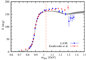
Within the elastic domain, the phase of our form factor $F_{+}(s)$ equals the scattering phase for the $P$ wave with $I$=1/2. From the expansion of the corresponding partial wave $t$-matrix near threshold we can obtain the threshold parameters. Following Ref. [48], they are defined for isospin $I$ and angular momentum $l$ as

where $q(s)$ is given by Eq. (6). It is simple to express our results in the form of Eq. (15) using

Then, using Eq. (24) and the results of Tab. 3 we can compute the threshold parameters. The first three of them are given in Tab. 6 for the four values of $s_{\rm cut}$ investigated in our main fit. The uncertainties in Tab. 6 are obtained from a MC that takes into account all errors and correlations given in Tabs. 3 and 4. One should however note that the functional form of the threshold parameters, unlike $\lambda_{+}^{\prime}$ and $\lambda_{+}^{\prime\prime}$, is determined by our model of $\delta(s)$. Their values depend mainly upon the masses and widths of the resonances, most notably that of the $K^{*}(892)$. Since the pole of the $K^{*}(892)$ is very well determined in our fits, the uncertainties in the scattering lengths are accordingly small. Tab. 6 contains only the propagation of statistical uncertainties. The systematics uncertainty associated with the threshold parameters will be estimated in Sec. 7.

In this section we present our final results. They are obtained from the main fit displayed in Tab. 3. Throughout this section, central values correspond to the average of the extrema found after the variation of $s_{\rm cut}$ in Tab. 3. Let us start with the mass and width of the $K^{*}(892)^{\pm}$. To the statistical uncertainty one should add another source of error: the imperfect knowledge of the detector response. To that end, we rely on the original analysis performed by the Belle collaboration where it is found to be 0.44 MeV for the mass of the $K^{*}(892)^{\pm}$ and 1.0 MeV for its width⁵⁵ 5 The determination of the error due to detector effects is rather involved and depends on the model that is assumed for the analysis. Therefore, we take these values as mere estimates [50]. [18]. In principle, one should include an uncertainty due to the residual dependence on $s_{\rm cut}$ but Tab. 3 shows that the results are almost invariant under changes of this parameter. Therefore, this source can safely be neglected. Our final results for the mass and width of the $K^{*}(892)^{\pm}$ defined from its pole position as in Eq. (9) are then

Before comparing this result with other analyses of the same data, one should note that in Refs. [18, 23] a different definition of the mass of the $K^{*}(892)^{\pm}$ was used. Therefore, we have computed the pole position for the other analyses in order to harmonise the definition of mass. Moreover, the use of Eq. (9) provides less model dependent results for the resonance parameters [36]. In Fig. 3, we compare the PDG recommended values $m_{K^{*}(892)^{\pm}}^{\rm PDG}=891.66\pm 0.26$ MeV and $\Gamma_{K^{*}(892)^{\pm}}^{\rm PDG}=50.8\pm 0.9$ MeV [41] with results for the mass and width of the $K^{*}(892)^{\pm}$ obtained from the pole position computed from the results of three different analyses of the Belle data set of $\tau\to K\pi\nu_{\tau}$ decays. Additional care should be taken when comparing these results since the PDG values are obtained chiefly from the parameters of Breit-Wigner-type expressions. On the basis of our results we claim that there is no tension between the mass found from $\tau$ decays and the PDG recommended value provided the pole position prescription is used for the former. On the other hand, the PDG value for the width is only marginally compatible with the one from Eq. (17). The width from analyses of the Belle data on $\tau\to K\pi\nu_{\tau}$ tend to lower values. Let us conclude by quoting another unambiguous result that can be derived from our analysis: the point $s_{\pi/2}$ satisfying $\delta(s_{\pi/2})=\pi/2$. Often, this point is used as the definition of the so-called visible or peak mass of a resonance since it is extracted from the direct comparison with experimental data⁶⁶ 6 If the resonance in question is narrow and isolated enough from other resonances and, furthermore, if no background is present, then the mass and width obtained in this way should be equal to the pole mass definition [36]. We observe that the pole mass is close but not the same as the peak mass. This is due to the fact that we are not in the ideal situation stated before.. In our fits, this value is also very stable with respect to changes in $s_{\rm cut}$ and reads

Our final values for $\lambda_{+}^{\prime}$ and $\lambda_{+}^{\prime\prime}$ come from the fits of Tab. 3. The results are again very stable with respect to changes in $s_{\rm cut}$. However, since now the statistical uncertainties are quite small, this model dependence contributes to the total error (specially in the case of $\lambda_{+}^{\prime\prime}$). From the mean of values of Tab. 3 we obtain

Concerning $\lambda_{+}^{\prime}$, Fig. 4 shows that the results from $K_{l_{3}}$ and $\tau\to K\pi\nu_{\tau}$ decays are in very good agreement⁷⁷ 7 For consistency we compare our results with dispersive analyses of $K_{l_{3}}$ decays. Data analyses that employ the quadratic Taylor expansion of Eq. (1) have much larger errors but agree as well with our numbers. For results from the quadratic form factor, see for instance [51] (ISTRA+), [52] (KLOE), [53] (NA48), and [54] (KTeV).. Our combined analysis produces a result in agreement with the others and with a rather small uncertainty. For $\lambda_{+}^{\prime\prime}$ the situation is somewhat different. Due to the restricted phase-space, quadratic fits of $K_{l_{3}}$ data do not provide a good determination of $\lambda_{+}^{\prime\prime}$ and dispersive analyses employ form factors with two subtractions, hence with only one subtraction constant determined directly from the data, namely $\lambda_{+}^{\prime}$. In Fig. 4, for $K_{l_{3}}$ experiments, we display results derived from the two-times subtracted form factor of Ref. [26]. We compare our results also to an average of analyses that employ Eq. (1) for $F_{+}$ [9]. Results from $\tau$ decay data have a better precision, and are compatible with results from $K_{l_{3}}$ experiments within their larger error bands.

From the expansion of Eq (4) we can calculate the third coefficient of a Taylor series of the type of Eq. (1) as

References

- [1] H. Leutwyler and M. Roos, Determination of the elements and of the Kobayashi-Maskawa matrix, Z. Physik C 25 (1984) 91.
- [2] M. Jamin, J. A. Oller and A. Pich, Light quark masses from scalar sum rules, Eur. Phys. J. C 24 (2002) 237 [hep-ph/0110194].
- [3] R. Appel et al. [E865 Collaboration], A large acceptance, high-resolution detector for rare decay experiments, Nucl. Instrum. Meth. A479 (2002) 349.
- [4] F. Bossi et al. [KLOE Collaboration], Precision kaon and hadron physics with KLOE, Riv. Nuovo Cim. 031, 531-623 (2008) [hep-ex/0811.1929].
- [5] N. Solomey [KTeV Collaboration], Development and performance of the KTeV transition radiation detector system, Nucl. Instrum. Meth. A419 (1998) 637.
- [6] V.N.Bolotov et al., Preprint IHEP 95-111, Protvino, 1995.
- [7] V. Fanti et al. [NA48 Collaboration], The Beam and detector for the NA48 neutral kaon CP violations experiment at CERN, Nucl. Instrum. Meth. A574 (2007) 433.
- [8] M. Antonelli et al. [FlaviaNet Working Group on Kaon Decays], Precision tests of the Standard Model with leptonic and semileptonic kaon decays, hep-ph/0801.1817.
- [9] M. Antonelli et al., An evaluation of and precise tests of the Standard Model from world data on leptonic and semileptonic kaon decays, \arXivid1005.2323.
- [10] E. Braaten, S. Narison, and A. Pich, QCD analysis of the hadronic width, Nucl. Phys. B 373 (1992) 581
- [11] P. A. Baikov, K. G. Chetyrkin and J. H. Kühn, Order QCD Corrections to and Decays, Phys. Rev. Lett. 101 (2008) 012002 [\arXivid0801.1821].
- [12] M. Davier, S. Descotes-Genon, A. Höcker, B. Malaescu, and Z. Zhang, The determination of from decays revisited, Eur. Phys. J. C 56 (2008) 305 [\arXivid0803.0979].
- [13] M. Beneke and M. Jamin, and the hadronic width: fixed-order, contour-improved and higher-order perturbation theory, J. High Energy Phys. 09 (2008) 044 [\arXivid0806.3156]
- [14] K. Maltman and T. Yavin, from hadronic decays, Phys. Rev. D 78 (2008) 094020 [\arXivid0807.0650]
- [15] R. Barate et al., Study of decays involving kaons, spectral functions and determination of the strange quark mass, Eur. Phys. J. C 11 (1999) 599 [hep-ex/9903015].
- [16] G. Abbiendi et al., Measurement of the strange spectral function in hadronic decays, Eur. Phys. J. C 35 (2004) 437 [hep-ex/0406007].
- [17] A. Lusiani,Tau decays at the B-factories, [\arXivid0905.1511].
- [18] D. Epifanov et al. [Belle Collaboration], Study of decay at Belle, Phys. Lett. B 654 (2007) 65 [\arXivid0706.2231]
- [19] S. Paramesvaran [BaBar Collaboration], proceedings of Meeting of the Division of Particles and Fields of the American Physical Society (DPF 2009), Detroit, Michigan, 26-31 Jul 2009, [\arXivid0910.2884].
- [20] D. M. Asner et al,Physics at BES-III, Edited by K. T. Chao and Y. F. Wang, Int. Int. J. Mod. Phys. A 24 (2009) 1 supp [\arXivid0809.1869].
- [21] M. Jamin, A. Pich and J. Portolés, Spectral distribution for the decay , Phys. Lett. B 640 (2006) 176 [hep-ph/0605096]
- [22] G. Ecker, J. Gasser, A. Pich and E. de Rafael, The role of resonances in chiral perturbation theory, Nucl. Phys. B 321 (1989) 311.
- [23] M. Jamin, A. Pich and J. Portolés, What can be learned from the Belle spectrum for the decay , Phys. Lett. B 664 (2008) 78 [\arXivid0803.1786].
- [24] D. R. Boito, R. Escribano and M. Jamin, vector form factor, dispersive constraints and decays, Eur. Phys. J. C 59 (2009) 821 [\arXivid0807.4883].
- [25] D. R. Boito, R. Escribano and M. Jamin, Dispersive representation of the vector form factor and fits to and data, PoS EFT09 (2009) 064 [\arXivid0904.0425]
- [26] V. Bernard, M. Oertel, E. Passemar and J. Stern, Dispersive representation and shape of the form factors: robustness, Phys. Rev. D 80 (2009) 034034 [\arXivid0903.1654].
- [27] E. Abouzaid et al. [ KTeV Collaboration ], Dispersive analysis of and scalar and vector form factors using KTeV data, Phys. Rev. D 81 (2010) 052001 [\arXivid0912.1291].
- [28] B. Moussallam, Analyticity constraints on the strangeness changing vector current and applications to , , Eur. Phys. J. C 53 (2008) 401 [\arXivid0710.0548].
- [29] M. Jamin, J. A. Oller and A. Pich, Strangeness-changing scalar form factors, Nucl. Phys. B 622 (2002) 279 [hep-ph/0110193].
- [30] M. Jamin, J. A. Oller and A. Pich, Order chiral couplings from the scalar form-factor, J. High Energy Phys. 02 (2004) 047 [hep-ph/0401080].
- [31] M. Jamin, J. A. Oller and A. Pich, Scalar form factor and light quark masses, Phys. Rev. D 74 (2006) 074009 [hep-ph/0605095].
- [32] V. Bernard, M. Oertel, E. Passemar and J. Stern, decay: A stringent test of right-handed quark currents, Phys. Lett. B 638 (2006) 480 [hep-ph/0603202].
- [33] G. Abbas, B. Ananthanarayan, I. Caprini, I. Sentitemsu Imsong and S. Ramanan, “Stringent constraints on the scalar form factor from analyticity, unitarity and low-energy theorems,” Eur. Phys. J. C 44 (2010) 175 [\arXivid0912.2831].
- [34] K. M. Watson, The effect of final state interactions on reaction cross-sections, Phys. Rev. D 88 (1952) 1163.
- [35] D. Epifanov, email communication.
- [36] R. Escribano, A. Gallegos, J. L. Lucio M, G. Moreno and J. Pestieau, On the mass, width and coupling constants of the , Eur. Phys. J. C 28 (2003) 107 [hep-ph/0204338].
- [37] J. J. Sanz-Cillero and A. Pich, meson properties in the Chiral Theory framework, Eur. Phys. J. C 27 (2003) 587 [hep-ph/0208199].
- [38] F. Guerrero and A. Pich, Effective field theory description of the pion form factor, Phys. Lett. B 412 (1997) 382 [hep-ph/9707347].
- [39] R. Omnès, On the solution of certain singular integral equations of Quantum Field Theory, Nuovo Cim. 8 (1958) 316.
- [40] A. Pich and J. Portolés, The vector form factor of the pion from unitarity and analyticity: a model-independent approach, Phys. Rev. D 63 (2001) 093005 [hep-ph/0101194].
- [41] C. Amsler et al. [Particle Data Group], The review of particle physics, Phys. Lett. B 667 (2008) 1.
- [42] J. Erler, Electroweak radiative corrections to semileptonic decays, Rev. Mex. Fis. 50, 200 (2004) [hep-ph/0211345].
- [43] J. L. Rosner and S. Stone, Leptonic decays of charged pseudoscalar mesons, [\arXivid1002.1655].
- [44] A. Wren, talk presented at Tau08, Novosibirsk, Russia. http://tau08.inp.nsk.su/talks/24/Wren.pdf
- [45] B. Aubert et al. [BABAR Collaboration], Measurement of using the BaBar detector, Nucl. Phys. B 189 (2009) 193 [\arXivid0808.1121].
- [46] D. Aston et al., A Study of scattering in the reaction at 11 GeV/c, Nucl. Phys. B 296 (1988) 493.
- [47] P. Estabrooks, R. K. Carnegie, A. D. Martin, W. M. Dunwoodie, T. A. Lasinski and D. W. G. Leith, Study of scattering using the reactions And at 13 GeV/c, Nucl. Phys. B 133 (1978) 490.
- [48] P. Büttiker, S. Descotes-Genon and B. Moussallam, A new analysis of scattering from Roy and Steiner type equations, Eur. Phys. J. C 33 (2004) 409 [hep-ph/0310283].
- [49] C. B. Lang and W. Porod, Symmetry breaking and the amplitudes in the unphysical region, Phys. Rev. D 21 (1980) 1295.
- [50] Simon Eidelman and Boris Shwartz, email communication.
- [51] O. P. Yushchenko et al., High statistic measurement of the decay form-factors, Phys. Lett. B 589 (2004) 111 [hep-ex/0404030].
- [52] F. Ambrosino et al. [KLOE Collaboration], Measurement of the form-factor parameters with the KLOE detector, J. High Energy Phys. 12 (2007) 105 [\arXivid0710.4470].
- [53] A. Lai et al. [NA48 Collaboration], Measurement of form factors, Phys. Lett. B 604 (2004) 1 [hep-ex/0410065].
- [54] T. Alexopoulos et al. [KTeV Collaboration], Measurements of semileptonic decay form factors, Phys. Rev. D 70 (2004) 092007 [hep-ex/0406003].
- [55] A. Lai et al. [NA48 Collaboration], Measurement of form factors, Phys. Lett. B 647 (2007) 341 [hep-ex/0703002].
- [56] The result from ISTRA+ can be found in Tab. 11 of Ref. [9]. The authors of Ref. [9] cite a communication by O. Yushchenko.
- [57] E. Passemar, Precision SM calculations and theoretical interests beyond the SM in and decays, PoS KAON09 (2009) 024 [\arXivid1003.4696].
- [58] J. Gasser, H. Leutwyler, Low-energy expansion of meson form-factors, Nucl. Phys. B 250 (1985) 517.
- [59] J. Bijnens and P. Talavera, “Pion and kaon electromagnetic form factors,” J. High Energy Phys. 03 (2002) 046 [hep-ph/0203049].
- [60] V. Bernard, N. Kaiser and, U. G. Meißner, scattering in chiral perturbation theory to one loop, Nucl. Phys. B 357 (1991) 129.
- [61] J. Bijnens, P. Dhonte and P. Talavera, scattering in three flavor ChPT, J. High Energy Phys. 05 (2004) 036 [hep-ph/0404150].
- [62] V. Bernard, N. Kaiser, U. G. Meißner, Chiral perturbation theory in the presence of resonances: application to and scattering, Nucl. Phys. B 364 (1991) 283.
- [63] M. Jamin, J. A. Oller and A. Pich, -wave scattering in chiral perturbation theory with resonances, Nucl. Phys. B 587 (2000) 331 [hep-ph/0006045].