跳到论文正文
W Papers独立论文阅读器 arXiv:1007.1852 论文正文 计算阅读时间 · 0%
引用这篇论文根据当前论文元数据生成,正式投稿前建议核对。


License: arXiv.org perpetual non-exclusive license
arXiv:1007.1852v2 [math.NA] 30 Nov 2010

A Generalized Sampling Theorem for Stable Reconstructions in Arbitrary Bases

Ben Adcock Affiliation: Department of Mathematics, Simon Fraser University,    Anders C. Hansen Affiliation: Department of Applied Mathematics and Theoretical Physics, University of Cambridge.
Abstract

We introduce a generalized framework for sampling and reconstruction in separable Hilbert spaces. Specifically, we establish that it is always possible to stably reconstruct a vector in an arbitrary Riesz basis from sufficiently many of its samples in any other Riesz basis. This framework can be viewed as an extension of that of Eldar et al. However, whilst the latter imposes stringent assumptions on the reconstruction basis, and may in practice be unstable, our framework allows for recovery in any (Riesz) basis in a manner that is completely stable.

Whilst the classical Shannon Sampling Theorem is a special case of our theorem, this framework allows us to exploit additional information about the approximated vector (or, in this case, function), for example sparsity or regularity, to design a reconstruction basis that is better suited. Examples are presented illustrating this procedure.

Keywords: Sampling Theory; Stable Reconstruction; Shannon Sampling Theorem; Infinite Matrices; Hilbert Space; Wavelets

00footnotetext: AMS classification:94A20, 65T99, 47A99, 42C40, 42A10

1 Introduction

The Shannon Sampling Theorem, or the Nyquist–Shannon Sampling Theorem as it is also called (we will refer to it as the NS-Sampling Theorem throughout the paper), is a mainstay in modern signal processing and has become one of the most important theorems in mathematics of information [26]. The list of applications of the theorem is long, and ranges from Magnetic Resonance Imaging (MRI) to sound engineering. We will in this paper address the question on whether or not the NS-Sampling Theorem can be improved. In particular, given the same set of information, could one design a reconstruction of a function that would be better than that provided by the NS-Sampling Theorem. The answer to such a question will obviously depend on the type of functions considered. However, suppose that we have some extra information about the functions to be reconstructed. One may, for example, have information about a basis that is particularly suited for such functions. Could this information be used to improve the reconstruction given by the NS-Sampling Theorem, even if it is based on the same sampling procedure? Although such a question has been posed before, and numerous extensions of the NS-Sampling Theorem have been developed [1, 2, 9, 10, 27], the generalization we introduce in this paper is, to the best of our knowledge, a novel approach for this problem.

The well known NS-Sampling Theorem [18, 20, 23, 24, 28] states that if

f=ℱg,g∈L(ℝ)2,f=\mathcal{F}g,\qquad g\in L{{}^{2}}(\mathbb{R}),

and supp⁡(g)⊂[−T,T]\mathrm{supp}(g)\subset[-T,T] for some T>0T>0, then both ff and gg can be reconstructed from point samples of ff. In particular, if ϵ≤12​T\epsilon\leq\frac{1}{2T} then

f⁡(t)=∑k=−∞∞f⁡(k​ϵ)​sinc​(t+k​ϵϵ)L​and unif. convergence,2f(t)=\sum_{k=-\infty}^{\infty}f(k\epsilon)\mathrm{sinc}\left(\frac{t+k\epsilon}{\epsilon}\right)\quad L{{}^{2}}\,\text{and unif. convergence,}
g(⋅)=ϵ∑k=−∞∞f(kϵ)e2πiϵk⋅L convergence.2g(\cdot)=\epsilon\sum_{k=-\infty}^{\infty}f(k\epsilon)e^{2\pi\mathrm{i}\epsilon k\cdot}\qquad L{{}^{2}}\text{ convergence.}

The quantity 12​T,\frac{1}{2T}, which is the largest value of ϵ\epsilon such that the theorem holds, is often referred to as the Nyquist rate [23]. In practice, when trying to reconstruct ff or gg, one will most likely not be able to access the infinite amount of information required, namely, {f⁡(k​ϵ)}k∈ℤ.\{f(k\epsilon)\}_{k\in\mathbb{Z}}. Moreover, even if we had access to all samples, we are limited by both processing power and storage to taking only a finite number. Thus, a more realistic scenario is that one will be given a finite number of samples {f⁡(k​ϵ)}|k|≤N\{f(k\epsilon)\}_{|k|\leq N}, for some N<∞N<\infty, and seek to reconstruct ff from these samples. The question is therefore: are the approximations

fN(⋅)=∑k=−NNf(kϵ)sinc(⋅+k​ϵϵ),gN(⋅)=ϵ∑k=−NNf(kϵ)e2πiϵk⋅f_{N}(\cdot)=\sum_{k=-N}^{N}f(k\epsilon)\mathrm{sinc}\left(\frac{\cdot+k\epsilon}{\epsilon}\right),\qquad g_{N}(\cdot)=\epsilon\sum_{k=-N}^{N}f(k\epsilon)e^{2\pi\mathrm{i}\epsilon k\cdot}

optimal for ff and gg given the information {f⁡(k​ϵ)}|k|≤N\{f(k\epsilon)\}_{|k|\leq N}? To formalize this question consider the following. For N∈ℕN\in\mathbb{N} and ϵ>0\epsilon>0, let

ΩN,ϵ={ξ∈ℂ2​N+1:ξ={f(kϵ)}|k|≤N,f∈L2(ℝ)∩C(ℝ)}.\begin{split}\Omega_{N,\epsilon}&=\{\xi\in\mathbb{C}^{2N+1}:\quad\xi=\{f(k\epsilon)\}_{|k|\leq N},\,f\in L^{2}(\mathbb{R})\cap C(\mathbb{R})\}.\end{split} (1.1)

(C⁡(ℝ)C(\mathbb{R}) denotes the set of continuous functions on ℝ\mathbb{R}). Define the mappings (with a slight abuse of notation)

ΛN,ϵ,1:ΩN,ϵ→L2​(ℝ),ΛN,ϵ,2:ΩN,ϵ→L2​(ℝ),\Lambda_{N,\epsilon,1}:\Omega_{N,\epsilon}\rightarrow L^{2}(\mathbb{R}),\quad\Lambda_{N,\epsilon,2}:\Omega_{N,\epsilon}\rightarrow L^{2}(\mathbb{R}),
ΛN,ϵ,1(f)=∑k=−NNf(kϵ)sinc(⋅+k​ϵϵ)ΛN,ϵ,2(f)=ϵ∑k=−NNf(kϵ)e2πiϵk⋅.\begin{split}\Lambda_{N,\epsilon,1}(f)=\sum_{k=-N}^{N}f(k\epsilon)\mathrm{sinc}\left(\frac{\cdot+k\epsilon}{\epsilon}\right)\qquad\Lambda_{N,\epsilon,2}(f)=\epsilon\sum_{k=-N}^{N}f(k\epsilon)e^{2\pi\mathrm{i}\epsilon k\cdot}.\end{split} (1.2)

The question is, given a class of functions Θ⊂L2​(ℝ)\Theta\subset L^{2}(\mathbb{R}), could there exist mappings ΞN,ϵ,1:ΩN,ϵ→L2​(ℝ)\Xi_{N,\epsilon,1}:\Omega_{N,\epsilon}\rightarrow L^{2}(\mathbb{R}) and ΞN,ϵ,2:ΩN,ϵ→L2​(ℝ)\Xi_{N,\epsilon,2}:\Omega_{N,\epsilon}\rightarrow L^{2}(\mathbb{R}) such that

‖ΞN,ϵ,1​(f)−f‖L∞​(ℝ)<‖ΛN,ϵ,1​(f)−f‖L∞​(ℝ)∀f,f=ℱ​g,g∈Θ,\begin{split}\|\Xi_{N,\epsilon,1}(f)-f\|_{L^{\infty}(\mathbb{R})}<\|\Lambda_{N,\epsilon,1}(f)-f\|_{L^{\infty}(\mathbb{R})}\quad\forall f,f=\mathcal{F}g,g\in\Theta,\end{split}
‖ΞN,ϵ,2​(f)−g‖L2​(ℝ)<‖ΛN,ϵ,2​(f)−g‖L2​(ℝ)∀f,f=ℱ​g,g∈Θ.\begin{split}\|\Xi_{N,\epsilon,2}(f)-g\|_{L^{2}(\mathbb{R})}<\|\Lambda_{N,\epsilon,2}(f)-g\|_{L^{2}(\mathbb{R})}\quad\forall f,f=\mathcal{F}g,g\in\Theta.\end{split}

As we will see later, the answer to this question may very well be yes, and the problem is therefore to find such mappings ΞN,ϵ,1\Xi_{N,\epsilon,1} and ΞN,ϵ,2.\Xi_{N,\epsilon,2}.

Refer to caption
Refer to caption
Figure 1: The figure shows ΛN,ϵ,2​(f)\Lambda_{N,\epsilon,2}(f) for f=ℱ​gf=\mathcal{F}g, N=500N=500 and ϵ=0.5\epsilon=0.5 (left) as well as gg (right).

As motivation for our work, consider the following reconstruction problem. Let gg be defined by

g⁡(t)={1t∈[0,1/2)−1t∈[1/2,1]0t∈ℝ∖[0,1].g(t)=\begin{cases}1&t\in[0,1/2)\\ -1&t\in[1/2,1]\\ 0&t\in\mathbb{R}\setminus[0,1].\end{cases}

This is the well-known Haar wavelet. Due to the discontinuity, there is no way one can exactly reconstruct this function with only finitely many function samples if one insists on using the mapping ΛN,ϵ,2\Lambda_{N,\epsilon,2}. We have visualized the reconstruction of gg using ΛN,ϵ,2\Lambda_{N,\epsilon,2} in Figure 1. In addition to gg not being reconstructed exactly, the approximation ΛN,ϵ,2​(g)\Lambda_{N,\epsilon,2}(g) is polluted by oscillations near the discontinuities of gg. Such oscillations are indicative of the well-known Gibbs phenomenon in recovering discontinuous signals from samples of their Fourier transforms [17]. This phenomenon is a major hurdle in many applications, including image and signal processing. Its resolution has, and continues to be, the subject of significant inquiry [25].

However, it is tempting to think that one could construct a mapping ΞN,ϵ,2\Xi_{N,\epsilon,2} that would yield a better result. Suppose for a moment that we do not know gg, but we do have some extra information. In particular, suppose that we know that g∈Θg\in\Theta, where

Θ={h∈L2​(ℝ):h=∑k=1Mβk​ψk},\Theta=\left\{h\in L^{2}(\mathbb{R}):h=\sum_{k=1}^{M}\beta_{k}\psi_{k}\right\}, (1.3)

for some finite number MM and where {ψk}\{\psi_{k}\} are the Haar wavelets on the interval [0,1].[0,1]. Could we, based on the extra knowledge of Θ\Theta, construct mappings ΞN,ϵ,1:ΩN,ϵ→L2​(ℝ)\Xi_{N,\epsilon,1}:\Omega_{N,\epsilon}\rightarrow L^{2}(\mathbb{R}) and ΞN,ϵ,2:ΩN,ϵ→L2​(ℝ)\Xi_{N,\epsilon,2}:\Omega_{N,\epsilon}\rightarrow L^{2}(\mathbb{R}) such that

sup{∥ΞN,ϵ,1(f)−f∥L∞​(ℝ):g∈Θ,f=ℱg}<sup{∥ΛN,ϵ,1(f)−f∥L∞​(ℝ):g∈Θ,f=ℱg},sup{∥ΞN,ϵ,2(f)−g∥L2​(ℝ):g∈Θ,f=ℱg}<sup{∥ΛN,ϵ,2(f)−g∥L2​(ℝ):g∈Θ,f=ℱg}?\begin{split}\sup\{\|\Xi_{N,\epsilon,1}(f)-f\|_{L^{\infty}(\mathbb{R})}:g\in\Theta,f=\mathcal{F}g\}&<\sup\{\|\Lambda_{N,\epsilon,1}(f)-f\|_{L^{\infty}(\mathbb{R})}:g\in\Theta,f=\mathcal{F}g\},\\ \sup\{\|\Xi_{N,\epsilon,2}(f)-g\|_{L^{2}(\mathbb{R})}:g\in\Theta,f=\mathcal{F}g\}&<\sup\{\|\Lambda_{N,\epsilon,2}(f)-g\|_{L^{2}(\mathbb{R})}:g\in\Theta,f=\mathcal{F}g\}?\end{split}

Indeed, this is the case, and a consequence of our framework is that it is possible to find ΞN,ϵ,1\Xi_{N,\epsilon,1} and ΞN,ϵ,2\Xi_{N,\epsilon,2} such that

sup{∥ΞN,ϵ,1(f)−f∥L∞​(ℝ):g∈Θ,f=ℱg}=0,sup{∥ΞN,ϵ,2(f)−g∥L2​(ℝ):g∈Θ,f=ℱg}=0,\begin{split}\sup\{\|\Xi_{N,\epsilon,1}(f)-f\|_{L^{\infty}(\mathbb{R})}:g\in\Theta,f=\mathcal{F}g\}&=0,\\ \sup\{\|\Xi_{N,\epsilon,2}(f)-g\|_{L^{2}(\mathbb{R})}:g\in\Theta,f=\mathcal{F}g\}&=0,\end{split}

provided NN is sufficiently large. In other words, one gets perfect reconstruction. Moreover, the reconstruction is done in a completely stable way.

The main tool for this task is a generalization of the NS-Sampling Theorem that allows reconstructions in arbitrary bases. Having said this, whilst the Shannon Sampling Theorem is the most standard example, the framework we develop addresses the more abstract problem of recovering a vector (belonging to some separable Hilbert space ℋ\mathcal{H}) given a finite number of its samples with respect any Riesz basis of ℋ\mathcal{H}.

1.1 Organization of the Paper

We have organized the paper as follows. In Section 2 we introduce notation and idea of finite sections of infinite matrices, a concept that will be crucial throughout the paper, and in Section 3 we discuss existing literature on this topic, including the work of Eldar et al [7, 8, 27]. The main theorem is presented and proved in Section 4, where we also show the connection to the classical NS-Sampling Theorem. The error bounds in the generalized sampling theorem involve several important constants, which can be estimated numerically. We therefore devote Section 5 to discussions on how to compute crucial constants and functions that are useful for providing error estimates. Finally, in Section 6 we provide several examples to support the generalized sampling theorem and to justify our approach.

2 Background and Notation

Let i\mathrm{i} denote the imaginary unit. Define the Fourier transform ℱ\mathcal{F} by

(ℱf)(y)=∫ℝdf(x)e−2πix⋅ydx,f∈L1(ℝd),(\mathcal{F}f)(y)=\int_{\mathbb{R}^{d}}f(x)e^{-2\pi\mathrm{i}x\cdot y}\,dx,\qquad f\in L^{1}(\mathbb{R}^{d}),

where, for vectors x,y∈ℝd,x,y\in\mathbb{R}^{d}, x⋅y=x1​y1+…+xd​yd.x\cdot y=x_{1}y_{1}+\ldots+x_{d}y_{d}. Aside from the Hilbert space L2​(ℝd)L^{2}(\mathbb{R}^{d}), we now introduce two other important Hilbert spaces: namely,

l2​(ℕ)={α={α1,α2,…}:∑k∈ℕ|αk2|<∞}l^{2}(\mathbb{N})=\left\{\alpha=\{\alpha_{1},\alpha_{2},\ldots\}:\sum_{k\in\mathbb{N}}|\alpha^{2}_{k}|<\infty\right\}

and

l2​(ℤ)={β={…​β−1,β0,β1​…}:∑k∈ℤ|βk2|<∞},l^{2}(\mathbb{Z})=\left\{\beta=\{\ldots\beta_{-1},\beta_{0},\beta_{1}\ldots\}:\sum_{k\in\mathbb{Z}}|\beta^{2}_{k}|<\infty\right\},

with their obvious inner products. We will also consider abstract Hilbert spaces. In this case we will use the notation ℋ\mathcal{H}. Note that {ej}j∈ℕ\{e_{j}\}_{j\in\mathbb{N}} and {ej}j∈ℤ\{e_{j}\}_{j\in\mathbb{Z}} will always denote the natural bases for l2​(ℕ)l^{2}(\mathbb{N}) and l2​(ℤ)l^{2}(\mathbb{Z}) respectively. We may also use the notation ℋ\mathcal{H} for both l2​(ℕ)l^{2}(\mathbb{N}) and l2​(ℤ)l^{2}(\mathbb{Z}) (the meaning will be clear from the context). Throughout the paper, the symbol ⊗\otimes will denote the standard tensor product on Hilbert spaces.

The concept of infinite matrices will be quite crucial in the theory, and also finite sections of such matrices. We will consider infinite matrices as operators from both l2​(ℕ)l^{2}(\mathbb{N}) to l2​(ℤ)l^{2}(\mathbb{Z}) and l2​(ℕ)l^{2}(\mathbb{N}) to l2​(ℕ)l^{2}(\mathbb{N}). The set of bounded operators from a Hilbert space ℋ1\mathcal{H}_{1} to a Hilbert space ℋ2\mathcal{H}_{2} will be denoted by ℬ⁡(ℋ1,ℋ2)\mathcal{B}(\mathcal{H}_{1},\mathcal{H}_{2}). As infinite matrices are unsuitable for computations we must reduce any infinite matrix to a more tractable finite-dimensional object. The standard means in which to do this is via finite sections. In particular, let

U=(⋰u−1,1u−1,2u−1,3…u0,1u0,2u0,3…u1,1u1,2u1,3…⋱),U∈ℬ⁡(l2​(ℕ),l2​(ℤ)).U=\left(\begin{matrix}\vdots&\vdots&\vdots&\iddots\\ u_{-1,1}&u_{-1,2}&u_{-1,3}&\ldots\\ u_{0,1}&u_{0,2}&u_{0,3}&\ldots\\ u_{1,1}&u_{1,2}&u_{1,3}&\ldots\\ \vdots&\vdots&\vdots&\ddots\\ \end{matrix}\right),\quad U\in\mathcal{B}(l^{2}(\mathbb{N}),l^{2}(\mathbb{Z})).

For n∈ℕn\in\mathbb{N}, define PnP_{n} to be the projection onto span⁡{e1,…,en}\mathrm{span}\{e_{1},\ldots,e_{n}\} and, for odd m∈ℕm\in\mathbb{N}, let P~m\widetilde{P}_{m} be the projection onto span⁡{e−m−12,…,em−12}\mathrm{span}\{e_{-\frac{m-1}{2}},\ldots,e_{\frac{m-1}{2}}\}. Then P~m​U​Pn\widetilde{P}_{m}UP_{n} may be interpreted as

(u−m−12,1…u−m−12,num−12,1…um−12,n),\left(\begin{matrix}u_{-\frac{m-1}{2},1}&\ldots&u_{-\frac{m-1}{2},n}\\ \vdots&\vdots&\vdots\\ u_{\frac{m-1}{2},1}&\ldots&u_{\frac{m-1}{2},n}\\ \end{matrix}\right),

a m×nm\times n finite section of UU. Finally, the spectrum of any operator T∈ℬ⁡(ℋ)T\in\mathcal{B}(\mathcal{H}) will be denoted by σ⁡(T).\sigma(T).

3 Connection to Earlier Work

The idea of reconstructing signals in arbitrary bases is certainly not a new idea and this topic has gone through extensive investigations in the last several decades. The papers by Unser and Aldroubi [1, 27] have been very influential and these ideas have been generalized to arbitrary Hilbert spaces by Eldar [7, 8]. The abstract framework introduced by Eldar is very powerful because of its general nature. Our framework is based on similar generalizations, yet it incorporates several key distinctions, resulting in a number of advantages. Before introducing this framework, let us first review some of the key concepts of [8].

Let ℋ\mathcal{H} be a separable Hilbert space and let f∈ℋf\in\mathcal{H} be an element we would like to reconstruct from some measurements. Suppose that we are given linearly independent sampling vectors {sk}k∈ℕ\{s_{k}\}_{k\in\mathbb{N}} that span a subspace 𝒮⊂ℋ\mathcal{S}\subset\mathcal{H} and form a Riesz basis, and assume that we can access the sampled inner products ck=⟨sk,f⟩c_{k}=\langle s_{k},f\rangle, k=1,2​…k=1,2\ldots. Suppose also that we are given linearly independent reconstruction vectors {wk}k∈ℕ\{w_{k}\}_{k\in\mathbb{N}} that span a subspace 𝒲⊂ℋ\mathcal{W}\subset\mathcal{H} and also form a Riesz basis. The task is to obtain a reconstruction f~∈𝒲\tilde{f}\in\mathcal{W} based on the sampling data {ck}k∈ℕ\{c_{k}\}_{k\in\mathbb{N}}. The natural choice, as suggested in [8], is

f~=W​(S∗​W)−1​S∗​f,\tilde{f}=W(S^{*}W)^{-1}S^{*}f, (3.1)

where the so-called synthesis operators S,W:l2​(ℕ)→ℋS,W:l^{2}(\mathbb{N})\rightarrow\mathcal{H} are defined by

S​x=x1​s1+x2​s2+…,W​y=y1​w1+y2​w2+…,Sx=x_{1}s_{1}+x_{2}s_{2}+\ldots,\qquad Wy=y_{1}w_{1}+y_{2}w_{2}+\ldots,

and their adjoints S∗,W∗:ℋ→l2​(ℕ)S^{*},W^{*}:\mathcal{H}\rightarrow l^{2}(\mathbb{N}) are easily seen to be

S∗​g={⟨s1,g⟩,⟨s2,g⟩,…},W∗​h={⟨w1,h⟩,⟨w2,h⟩​…}.S^{*}g=\{\langle s_{1},g\rangle,\langle s_{2},g\rangle,\ldots\},\qquad W^{*}h=\{\langle w_{1},h\rangle,\langle w_{2},h\rangle\ldots\}.

Note that S∗​WS^{*}W will be invertible if and only if

ℋ=𝒲⊕𝒮⟂.\mathcal{H}=\mathcal{W}\oplus\mathcal{S}^{\perp}.

This gives a very nice and intuitive abstract formulation of the reconstruction. However, in practice we will never have the luxury of being able to acquire nor process the infinite amount of samples ⟨sk,f⟩\langle s_{k},f\rangle, k=1,2​…k=1,2\ldots, needed to construct f~\tilde{f}. An important question to ask is therefore:

  • What if we are given only the first m∈ℕm\in\mathbb{N} samples ⟨sk,f⟩\langle s_{k},f\rangle, k=1,…,mk=1,\ldots,m? In this case we cannot use (3.1), and we may ask: what to do?

Fortunately, there is a simple finite dimensional analog to the infinite dimensional ideas discussed above. Suppose that we are given m∈ℕm\in\mathbb{N} linearly independent sampling vectors {s1,…,sm}\{s_{1},\ldots,s_{m}\} that span a subspace 𝒮m⊂ℋ\mathcal{S}_{m}\subset\mathcal{H}, and assume that we can access the sampled inner products ck=⟨sk,f⟩c_{k}=\langle s_{k},f\rangle, k=1,…,mk=1,\ldots,m. Suppose also that we are given linearly independent reconstruction vectors {w1,…,wm}\{w_{1},\ldots,w_{m}\} that span a subspace 𝒲m⊂ℋ\mathcal{W}_{m}\subset\mathcal{H}. The task is to construct an approximation f~∈𝒲m\tilde{f}\in\mathcal{W}_{m} to ff based on the samples {ck}k=1m.\{c_{k}\}_{k=1}^{m}. In particular, we are interested in finding coefficients {dk}k=1m\{d_{k}\}_{k=1}^{m} (that are computed from the samples {ck}k=1m\{c_{k}\}_{k=1}^{m}) such that f~=∑k=1mdk​wk\tilde{f}=\sum_{k=1}^{m}d_{k}w_{k}. The reconstruction suggested in [6] is

f~=∑k=1mdk​wk=Wm​(Sm∗​Wm)−1​Sm∗​f,\tilde{f}=\sum_{k=1}^{m}d_{k}w_{k}=W_{m}(S_{m}^{*}W_{m})^{-1}S_{m}^{*}f, (3.2)

where the operators Sm,Wm:ℂm→ℋS_{m},W_{m}:\mathbb{C}^{m}\rightarrow\mathcal{H} are defined by

Sm​x=x1​s1+…+xm​sm,Wm​y=y1​w1+…+ym​wm,S_{m}x=x_{1}s_{1}+\ldots+x_{m}s_{m},\qquad W_{m}y=y_{1}w_{1}+\ldots+y_{m}w_{m}, (3.3)

and their adjoints S∗,W∗:ℋ→ℂmS^{*},W^{*}:\mathcal{H}\rightarrow\mathbb{C}^{m} are easily seen to be

Sm∗​g={⟨s1,g⟩,…,⟨sm,g⟩},Wm∗​h={⟨w1,h⟩,…,⟨wm,h⟩}.S_{m}^{*}g=\{\langle s_{1},g\rangle,\ldots,\langle s_{m},g\rangle\},\qquad W_{m}^{*}h=\{\langle w_{1},h\rangle,\ldots,\langle w_{m},h\rangle\}.

From this it is clear that we can express Sm∗​Wm:ℂm→ℂmS_{m}^{*}W_{m}:\mathbb{C}^{m}\rightarrow\mathbb{C}^{m} as the matrix

(⟨s1,w1⟩…⟨s1,wm⟩⟨sm,w1⟩…⟨sm,wm⟩).\left(\begin{matrix}\langle s_{1},w_{1}\rangle&\ldots&\langle s_{1},w_{m}\rangle\\ \vdots&\vdots&\vdots\\ \langle s_{m},w_{1}\rangle&\ldots&\langle s_{m},w_{m}\rangle\\ \end{matrix}\right). (3.4)

Also, Sm∗​WmS_{m}^{*}W_{m} is invertible if and only if and ([6, Prop. 3])

𝒲m∩𝒮m⟂={0}.\mathcal{W}_{m}\cap\mathcal{S}_{m}^{\perp}=\{0\}. (3.5)

Thus, to construct f~\tilde{f} one simply solves a linear system of equations. The error can now conveniently be bounded from above and below by

‖f−P𝒲m​f‖≤‖f−f~‖≤1cos⁡(θ𝒲m​𝒮m)​‖f−P𝒲m​f‖,\|f-P_{\mathcal{W}_{m}}f\|\leq\|f-\tilde{f}\|\leq\frac{1}{\cos(\theta_{\mathcal{W}_{m}\mathcal{S}_{m}})}\|f-P_{\mathcal{W}_{m}}f\|,

where P𝒲mP_{\mathcal{W}_{m}} is the projection onto 𝒲m\mathcal{W}_{m},

cos(θ𝒲m​𝒮m)=inf{∥P𝒮mg∥:g∈𝒲m,∥g∥=1}\cos(\theta_{\mathcal{W}_{m}\mathcal{S}_{m}})=\mathrm{inf}\{\|P_{\mathcal{S}_{m}}g\|:g\in\mathcal{W}_{m},\|g\|=1\}

is the cosine of the angles between the subspaces 𝒮m\mathcal{S}_{m} and 𝒲m\mathcal{W}_{m} and P𝒮mP_{\mathcal{S}_{m}} is the projection onto 𝒮m\mathcal{S}_{m} [6]. Note that if f∈𝒲mf\in\mathcal{W}_{m}, then f~=f\tilde{f}=f exactly, a feature known as perfect recovery. Another facet of this framework is so-called consistency: the samples ⟨sj,f~⟩\langle s_{j},\tilde{f}\rangle, j=1,…,mj=1,\ldots,m, of the approximation f~\tilde{f} are identical to those of the original function ff (indeed, f~\tilde{f}, as given by (3.2), can be equivalently defined as the unique element in 𝒲m\mathcal{W}_{m} that is consistent with ff).

Returning to this issue at hand, there are now several important questions to ask:

  • (i)

    What if 𝒲m∩𝒮m⟂≠{0}\mathcal{W}_{m}\cap\mathcal{S}_{m}^{\perp}\neq\{0\} so that Sm∗​WmS_{m}^{*}W_{m} is not invertible? It is very easy to construct theoretical examples such that Sm∗​WmS_{m}^{*}W_{m} is not invertible, however (as we will see below), such situations may very well occur in applications. In fact, 𝒲m∩𝒮m⟂={0}\mathcal{W}_{m}\cap\mathcal{S}_{m}^{\perp}=\{0\} is a rather strict condition. If we have that 𝒲m∩𝒮m⟂≠{0}\mathcal{W}_{m}\cap\mathcal{S}_{m}^{\perp}\neq\{0\} does that mean that is is impossible to construct an approximation f~\tilde{f} from the samples Sm∗​fS_{m}^{*}f?

  • (ii)

    What if ‖(Sm∗​Wm)−1‖\|(S_{m}^{*}W_{m})^{-1}\| is large? The stability of the method must clearly depend on the quantity ‖(Sm∗​Wm)−1‖\|(S_{m}^{*}W_{m})^{-1}\|. Thus, even if (Sm∗​Wm)−1(S_{m}^{*}W_{m})^{-1} exists, one may not be able to use the method in practice as there will likely be increased sensitivity to both round-off error and noise.

Our framework is specifically designed to tackle these issues. But before we present our idea, let us consider some examples where the issues in (i) and (ii) will be present.

Refer to caption
Refer to caption
Figure 2: This figure shows log10⁡‖(Sϵ,m∗​Wm)−1‖\log_{10}\|(S^{*}_{\epsilon,m}W_{m})^{-1}\| as a function of mm and ϵ\epsilon for m=1,2,…,100m=1,2,\ldots,100. The left plot corresponds to ϵ=1\epsilon=1, whereas the right plot corresponds to ϵ=7/8\epsilon=7/8 (circles), ϵ=1/2\epsilon=1/2 (crosses) and ϵ=1/8\epsilon=1/8 (diamonds).
Example 3.1.

As for (i), the simplest example is to let ℋ=l2​(ℤ)\mathcal{H}=l^{2}(\mathbb{Z}) and {ej}j∈ℤ\{e_{j}\}_{j\in\mathbb{Z}} be the natural basis (eje_{j} is the infinite sequence with 11 in its jj-th coordinate and zeros elsewhere). For m∈ℕm\in\mathbb{N}, let the sampling vectors {sk}k=−mm\{s_{k}\}_{k=-m}^{m} and the reconstruction vectors {wk}k=−mm\{w_{k}\}_{k=-m}^{m} be defined by sk=eks_{k}=e_{k} and wk=ek+1.w_{k}=e_{k+1}. Then, clearly, 𝒲m∩𝒮m⟂=span⁡{em+1}\mathcal{W}_{m}\cap\mathcal{S}_{m}^{\perp}=\mathrm{span}\{e_{m+1}\}.

Example 3.2.

For an example of more practical interest, consider the following: For 0<ϵ≤10<\epsilon\leq 1 let ℋ=L2​([0,1/ϵ])\mathcal{H}=L^{2}([0,1/\epsilon]), and, for odd m∈ℕm\in\mathbb{N}, define the sampling vectors

{sϵ,k}k=−(m−1)/2(m−1)/2,sϵ,k=e−2πiϵk⋅χ[0,1/ϵ],\{s_{\epsilon,k}\}_{k=-(m-1)/2}^{(m-1)/2},\qquad s_{\epsilon,k}=e^{-2\pi\mathrm{i}\epsilon k\cdot}\chi_{[0,1/\epsilon]},

(this is exactly the type of measurement vector that will be used if one models Magnetic Resonance Imaging) and let the reconstruction vectors {wk}k=1m\{w_{k}\}_{k=1}^{m} denote the mm first Haar wavelets on [0,1][0,1] (including the constant function, w1=χ[0,1]w_{1}=\chi_{[0,1]}). Let Sϵ,mS_{\epsilon,m} and WmW_{m} be as in (3.3), according to the sampling and reconstruction vectors just defined. A plot of ‖(Sϵ,m∗​Wm)−1‖\|(S_{\epsilon,m}^{*}W_{m})^{-1}\| as a function of mm and ϵ\epsilon is given in Figure 2. As we observe, for ϵ=1\epsilon=1 only certain values of mm yield stable reconstruction, whereas for the other values of ϵ\epsilon the quantity ‖(Sϵ,m∗​Wm)−1‖\|(S_{\epsilon,m}^{*}W_{m})^{-1}\| grows exponentially with mm, making the problem severely ill-conditioned. Further computations suggest that ‖(Sϵ,m∗​Wm)−1‖\|(S_{\epsilon,m}^{*}W_{m})^{-1}\| increases exponentially with mm not just for these values of ϵ\epsilon, but for all 0<ϵ<1.0<\epsilon<1.

Example 3.3.

Another example can be made by replacing the Haar wavelet basis with the basis consisting of Legendre polynomials (orthogonal polynomials on [−1,1][-1,1] with respect to the Euclidean inner product).

In Figure 3 we plot the quantity ‖(Sϵ,m∗​Wm)−1‖\|(S_{\epsilon,m}^{*}W_{m})^{-1}\|. Unlike the previous example, this quantity grows exponentially and monotonically in mm. Whilst this not only makes the method highly susceptible to round-off error and noise, it can also prevent convergence of the approximation f~\tilde{f} (as m→∞m\rightarrow\infty). In essence, for convergence to occur, the error ‖f−P𝒲m​f‖\|f-P_{\mathcal{W}_{m}}f\| must decay more rapidly than the quantity ‖(Sϵ,m∗​Wm)−1‖\|(S_{\epsilon,m}^{*}W_{m})^{-1}\| grows. Whenever this is not the case, convergence is not assured. To illustrate this shortcoming, in Figure 3 we also plot the error ‖f−f~‖\|f-\tilde{f}\|, where f⁡(x)=11+16​x2f(x)=\frac{1}{1+16x^{2}}. The complex singularity at x=±14​ix=\pm\frac{1}{4}\mathrm{i} limits the convergence rate of ‖f−P𝒲m​f‖\|f-P_{\mathcal{W}_{m}}f\| sufficiently so that f~\tilde{f} does not converge to ff. Note that this effect is well documented as occurring in a related reconstruction problem, where a function defined on [−1,1][-1,1] is interpolated at mm equidistant pointwise samples by a polynomial of degree m−1m-1. This is the famous Runge phenomenon. The problem considered above (reconstruction from mm Fourier samples) can be viewed as a continuous analogue of this phenomenon.

Refer to caption
Refer to caption
Figure 3: The left figure shows log10⁡‖(Sϵ,m∗​Wm)−1‖\log_{10}\|(S_{\epsilon,m}^{*}W_{m})^{-1}\| as a function of mm for m=2,4,…,50m=2,4,\ldots,50 and ϵ=1,78,12,18\epsilon=1,\frac{7}{8},\frac{1}{2},\frac{1}{8} (squares, circles, crosses and diamonds respectively). The right figure shows log10⁡‖f−P𝒲m​f‖\log_{10}\|f-P_{\mathcal{W}_{m}}f\| (squares) and log10⁡‖f−f~‖\log_{10}\|f-\tilde{f}\| (circles) for m=2,4,6,…,100m=2,4,6,\ldots,100, where f⁡(x)=11+16​x2f(x)=\frac{1}{1+16x^{2}}.

Actually, the phenomenon illustrated in Examples 3.2 and 3.3 is not hard to explain if one looks at the problem from an operator-theoretical point of view. This is the topic of the next section.

3.1 Connections to the Finite Section Method

To illustrate the idea, let {sk}k∈ℕ\{s_{k}\}_{k\in\mathbb{N}} and {wk}k∈ℕ\{w_{k}\}_{k\in\mathbb{N}} be two sequences of linearly independent elements in a Hilbert space ℋ\mathcal{H}. Define the infinite matrix UU by

U=(u11u12u13…u21u22u23…u31u32u33…⋱),ui​j=⟨si,wj⟩.U=\left(\begin{matrix}u_{11}&u_{12}&u_{13}&\ldots\\ u_{21}&u_{22}&u_{23}&\ldots\\ u_{31}&u_{32}&u_{33}&\ldots\\ \vdots&\vdots&\vdots&\ddots\\ \end{matrix}\right),\qquad u_{ij}=\langle s_{i},w_{j}\rangle. (3.6)

Thus, by (3.4) the operator Sm∗​WmS_{m}^{*}W_{m} is simply the mm by mm finite section of UU. In particular

Sm∗​Wm=Pm​U​Pm|Pm​l2​(ℕ).S_{m}^{*}W_{m}=P_{m}UP_{m}|_{P_{m}l^{2}(\mathbb{N})}.

The finite section method has been studied extensively for the last decades [3, 12, 13, 21]. It is well known that even if UU is invertible then Pm​U​Pm|Pm​l2​(ℕ)P_{m}UP_{m}|_{P_{m}l^{2}(\mathbb{N})} may never be invertible for any mm. In fact one must have rather strict conditions on UU for Pm​U​Pm|Pm​l2​(ℕ)P_{m}UP_{m}|_{P_{m}l^{2}(\mathbb{N})} to be invertible with uniformly bounded inverse (such as positive self-adjointness, for example [21]). In addition, even if U:l2​(ℕ)→l2​(ℕ)U:l^{2}(\mathbb{N})\rightarrow l^{2}(\mathbb{N}) is invertible and Pm​U​Pm|Pm​l2​(ℕ)P_{m}UP_{m}|_{P_{m}l^{2}(\mathbb{N})} is invertible for all m∈ℕ,m\in\mathbb{N}, it may be the case that, if

x=U−1​y,x,y∈l2​(ℕ),xm=(Pm​U​Pm|Pm​l2​(ℕ))−1​Pm​yx=U^{-1}y,\quad x,y\in l^{2}(\mathbb{N}),\qquad x_{m}=(P_{m}UP_{m}|_{P_{m}l^{2}(\mathbb{N})})^{-1}P_{m}y

then

xm↛x,m→∞.x_{m}\nrightarrow x,\qquad m\rightarrow\infty.

Suppose that {sk}k∈ℕ\{s_{k}\}_{k\in\mathbb{N}} and {wk}k∈ℕ\{w_{k}\}_{k\in\mathbb{N}} are two Riesz bases for closed subspaces 𝒮\mathcal{S} and 𝒲\mathcal{W} of a separable Hilbert space ℋ\mathcal{H}. Define the operators S,W:l2​(ℕ)→ℋS,W:l^{2}(\mathbb{N})\rightarrow\mathcal{H} by

S​x=x1​s1+x2​s2+…,W​y=y1​w1+y2​w2+….Sx=x_{1}s_{1}+x_{2}s_{2}+\ldots,\qquad Wy=y_{1}w_{1}+y_{2}w_{2}+\ldots. (3.7)

Suppose now that (S∗​W)−1(S^{*}W)^{-1} exists. For m∈ℕm\in\mathbb{N}, let the spaces 𝒮m,𝒲m\mathcal{S}_{m},\mathcal{W}_{m} and operators Sm,Wm:ℂm→ℋS_{m},W_{m}:\mathbb{C}^{m}\rightarrow\mathcal{H} be defined as in Section 3 according to the vectors {sk}k=1m\{s_{k}\}_{k=1}^{m} and {wk}k=1m\{w_{k}\}_{k=1}^{m} respectively. The following scenarios may now arise:

  • (i)

    𝒲∩𝒮⟂={0}\mathcal{W}\cap\mathcal{S}^{\perp}=\{0\}, yet

    𝒲m∩𝒮m⟂≠{0},∀m∈ℕ.\mathcal{W}_{m}\cap\mathcal{S}^{\perp}_{m}\neq\{0\},\qquad\forall\,m\in\mathbb{N}.
  • (ii)

    ‖(S∗​W)−1‖<∞\|(S^{*}W)^{-1}\|<\infty and the inverse (Sm∗​Wm)−1(S_{m}^{*}W_{m})^{-1} exists for all m∈ℕm\in\mathbb{N}, but

    ‖(Sm∗​Wm)−1‖⟶∞,m→∞.\|(S_{m}^{*}W_{m})^{-1}\|\longrightarrow\infty,\qquad m\rightarrow\infty.
  • (iii)

    (Sm∗​Wm)−1(S_{m}^{*}W_{m})^{-1} exists for all m∈ℕ,m\in\mathbb{N}, however

    Wm​(Sm∗​Wm)−1​Sm∗​f↛f,m→∞,W_{m}(S_{m}^{*}W_{m})^{-1}S_{m}^{*}f\nrightarrow f,\qquad m\rightarrow\infty,

    for some f∈𝒲f\in\mathcal{W}.

Thus, in order for us to have a completely general sampling theorem we must try to extend the framework described in this section in order to overcome the obstacles listed above.

4 The New Approach

4.1 The Idea

One would like to have a completely general sampling theory that can be described as follows:

  • (i)

    We have a signal f∈ℋf\in\mathcal{H} and a Riez basis {wk}k∈ℕ\{w_{k}\}_{k\in\mathbb{N}} that spans some closed subspace 𝒲⊂ℋ\mathcal{W}\subset\mathcal{H}, and

    f=∑k=1∞βk​wk,βk∈ℂ.f=\sum_{k=1}^{\infty}\beta_{k}w_{k},\qquad\beta_{k}\in\mathbb{C}.

    So f∈𝒲f\in\mathcal{W} (we may also typically have some information on the decay rate of the βk\beta_{k}s, however, this is not crucial for our theory).

  • (ii)

    We have sampling vectors {sk}k∈ℕ\{s_{k}\}_{k\in\mathbb{N}} that form a Riez basis for a closed subspace 𝒮⊂ℋ,\mathcal{S}\subset\mathcal{H}, (note that we may not have the luxury of choosing such sampling vectors as they may be specified by some particular model, as is the case in MRI) and we can access the sampling values {⟨sk,f⟩}k∈ℕ.\{\langle s_{k},f\rangle\}_{k\in\mathbb{N}}.

Goal: reconstruct the best possible approximation f~∈𝒲\tilde{f}\in\mathcal{W} based on the finite subset {⟨sk,f⟩}k=1m\{\langle s_{k},f\rangle\}_{k=1}^{m} of the sampling information {⟨sk,f⟩}k∈ℕ\{\langle s_{k},f\rangle\}_{k\in\mathbb{N}}.

We could have chosen mm vectors {w1,…,wm}\{w_{1},\ldots,w_{m}\} and defined the operators SmS_{m} and WmW_{m} as in (3.3) (from {w1,…,wm}\{w_{1},\ldots,w_{m}\} and {s1,…,sm}\{s_{1},\ldots,s_{m}\}) and let f~\tilde{f} be defined by (3.2). However, this may be impossible as Sm∗​WmS_{m}^{*}W_{m} may not be invertible (or the inverse may have a very large norm), as discussed in Examples 3.2 and 3.3. The question is then: what to do?

To deal with these issues we will launch an abstract sampling theorem that extends the ideas discussed above. To do so, we first notice that, since {sj}\{s_{j}\} and {wj}\{w_{j}\} are Riesz bases, there exist constants A,B,C,D>0A,B,C,D>0 such that

A​∑k∈ℕ|αk|2≤‖∑k∈ℕαk​wk‖2≤B​∑k∈ℕ|αk|2C∑k∈ℕ|αk|2≤‖∑k∈ℕαksk‖2≤D∑k∈ℕ|αk|2,∀{α1,α2,…}∈l2(ℕ).\begin{split}&A\sum_{k\in\mathbb{N}}|\alpha_{k}|^{2}\leq\left\|\sum_{k\in\mathbb{N}}\alpha_{k}w_{k}\right\|^{2}\leq B\sum_{k\in\mathbb{N}}|\alpha_{k}|^{2}\\ &C\sum_{k\in\mathbb{N}}|\alpha_{k}|^{2}\leq\left\|\sum_{k\in\mathbb{N}}\alpha_{k}s_{k}\right\|^{2}\leq D\sum_{k\in\mathbb{N}}|\alpha_{k}|^{2},\quad\forall\,\{\alpha_{1},\alpha_{2},\ldots\}\in l^{2}(\mathbb{N}).\end{split} (4.1)

Now let UU be defined as in (3.6). Instead of dealing with Pm​U​Pm|Pm​l2​(ℕ)=Sm∗​WmP_{m}UP_{m}|_{P_{m}l^{2}(\mathbb{N})}=S_{m}^{*}W_{m} we propose to choose n∈ℕn\in\mathbb{N} and compute the solution {β~1,…,β~n}\{\tilde{\beta}_{1},\ldots,\tilde{\beta}_{n}\} of the following equation:

A(β~1β~2β~n)=PnU∗Pm(⟨s1,f⟩⟨s2,f⟩⟨sm,f⟩),A=PnU∗PmUPn|Pn​ℋ,A\left(\begin{matrix}\tilde{\beta}_{1}\\ \tilde{\beta}_{2}\\ \vdots\\ \tilde{\beta}_{n}\\ \end{matrix}\right)=P_{n}U^{*}P_{m}\left(\begin{matrix}\langle s_{1},f\rangle\\ \langle s_{2},f\rangle\\ \vdots\\ \langle s_{m},f\rangle\\ \end{matrix}\right),\qquad A=P_{n}U^{*}P_{m}UP_{n}\lvert_{P_{n}\mathcal{H}}, (4.2)

provided a solution exists (later we will provide estimates on the size of n,mn,m for (4.2) to have a unique solution). Finally we let

f~=∑k=1nβ~k​wk.\tilde{f}=\sum_{k=1}^{n}\tilde{\beta}_{k}w_{k}. (4.3)

Note that, for n=mn=m this is equivalent to (3.2), and thus we have simply extended the framework discussed in Section 3. However, for m>nm>n this is no longer the case. As we later establish, allowing mm to range independently of nn is the key to the advantage possessed by this framework.

Before doing so, however, we first mention that the framework proposed above differs from that discussed previously in that it is inconsistent. Unlike (3.2), the samples ⟨sj,f~⟩\langle s_{j},\tilde{f}\rangle do not coincide with those of the function ff. Yet, as we shall now see, by dropping the requirement of consistency, we obtain a reconstruction which circumvents the aforementioned issues associated with (3.2).

4.2 The Abstract Sampling Theorem

The task is now to analyze the model in (4.2) by both establishing existence of f~\tilde{f} and providing error bounds for ‖f−f~‖\|f-\tilde{f}\|. We have

Theorem 4.1.

Let ℋ\mathcal{H} be a separable Hilbert space and 𝒮,𝒲⊂ℋ\mathcal{S},\mathcal{W}\subset\mathcal{H} be closed subspaces such that 𝒲∩𝒮⟂={0}\mathcal{W}\cap\mathcal{S}^{\perp}=\{0\}. Suppose that {sk}k∈ℕ\{s_{k}\}_{k\in\mathbb{N}} and {wk}k∈ℕ\{w_{k}\}_{k\in\mathbb{N}} are Riesz bases for 𝒮\mathcal{S} and 𝒲\mathcal{W} respectively with constants A,B,C,D>0A,B,C,D>0. Suppose that

f=∑k∈ℕβkwk,β={β1,β2,…,}∈l2(ℕ).f=\sum_{k\in\mathbb{N}}\beta_{k}w_{k},\qquad\beta=\{\beta_{1},\beta_{2},\ldots,\}\in l^{2}(\mathbb{N}). (4.4)

Let n∈ℕn\in\mathbb{N}. Then there is an M∈ℕM\in\mathbb{N} (in particular M=min{k:0∉σ(PnU∗PkUPn|Pn​ℋ)}M=\min\{k:0\notin\sigma(P_{n}U^{*}P_{k}UP_{n}\lvert_{P_{n}\mathcal{H}})\}) such that, for all m≥Mm\geq M, the solution {β~1,…,β~n}\{\tilde{\beta}_{1},\ldots,\tilde{\beta}_{n}\} to (4.2) is unique. Also, if f~\tilde{f} is as in (4.3), then

‖f−f~‖ℋ≤B​(1+Kn,m)​‖Pn⟂​β‖l2​(ℕ),\|f-\tilde{f}\|_{\mathcal{H}}\leq\sqrt{B}(1+K_{n,m})\|P_{n}^{\perp}\beta\|_{l^{2}(\mathbb{N})}, (4.5)

where

Kn,m=‖(PnU∗PmUPn|Pn​ℋ)−1PnU∗PmUPn⟂‖.K_{n,m}=\left\|(P_{n}U^{*}P_{m}UP_{n}\lvert_{P_{n}\mathcal{H}})^{-1}P_{n}U^{*}P_{m}UP_{n}^{\perp}\right\|. (4.6)

The theorem has an immediate corollary that is useful for estimating the error. We have

Corollary 4.2.

With the same assumptions as in Theorem 4.1 and fixed n∈ℕn\in\mathbb{N},

‖(PnU∗PmUPn|Pn​ℋ)−1‖⟶‖(PnU∗UPn|Pn​ℋ)−1‖≤‖(U∗U)−1‖≤1A​C,m→∞.\left\|(P_{n}U^{*}P_{m}UP_{n}\lvert_{P_{n}\mathcal{H}})^{-1}\right\|\longrightarrow\left\|(P_{n}U^{*}UP_{n}\lvert_{P_{n}\mathcal{H}})^{-1}\right\|\leq\left\|(U^{*}U)^{-1}\right\|\leq\frac{1}{AC},\quad m\rightarrow\infty. (4.7)

In addition, if UU is an isometry (in particular, when {wk}k∈ℕ,{sk}k∈ℕ\{w_{k}\}_{k\in\mathbb{N}},\{s_{k}\}_{k\in\mathbb{N}} are orthonormal) then it follows that

Kn,m⟶0,m→∞.K_{n,m}\longrightarrow 0,\qquad m\rightarrow\infty.
Proof of Theorem 4.1.

Let UU be as in as in (3.6). Then (4.4) yields the following infinite system of equations:

(⟨s1,f⟩⟨s2,f⟩⟨s3,f⟩)=(u11u12u13…u21u22u23…u31u32u33…⋱)​(β1β2β3).\left(\begin{matrix}\langle s_{1},f\rangle\\ \langle s_{2},f\rangle\\ \langle s_{3},f\rangle\\ \vdots\\ \end{matrix}\right)=\left(\begin{matrix}u_{11}&u_{12}&u_{13}&\ldots\\ u_{21}&u_{22}&u_{23}&\ldots\\ u_{31}&u_{32}&u_{33}&\ldots\\ \vdots&\vdots&\vdots&\ddots\\ \end{matrix}\right)\left(\begin{matrix}\beta_{1}\\ \beta_{2}\\ \beta_{3}\\ \vdots\\ \end{matrix}\right). (4.8)

Note that UU must be a bounded operator. Indeed, let SS and WW be as in (3.7). Since

⟨S∗​W​ej,ei⟩=⟨si,wj⟩,i,j∈ℕ,\langle S^{*}We_{j},e_{i}\rangle=\langle s_{i},w_{j}\rangle,\qquad i,j\in\mathbb{N},

it follows that U=S∗​WU=S^{*}W. However, from (4.1) we find that both WW and SS are bounded as mappings from l2​(ℕ)l^{2}(\mathbb{N}) onto 𝒲\mathcal{W} and 𝒮\mathcal{S} respectively, with ‖W‖≤B\|W\|\leq\sqrt{B}, ‖S‖≤D\|S\|\leq\sqrt{D}, thus yielding our claim. Note also that, by the assumption that 𝒲∩𝒮⟂={0}\mathcal{W}\cap\mathcal{S}^{\perp}=\{0\}, (4.8) has a unique solution. Indeed, since 𝒲∩𝒮⟂={0}\mathcal{W}\cap\mathcal{S}^{\perp}=\{0\} it follows that inf‖x‖=1‖S∗​W​x‖≠0\inf_{\|x\|=1}\|S^{*}Wx\|\neq 0, so UU must be injective.

Now let ηf={⟨s1,f⟩,⟨s1,f⟩,…}\eta_{f}=\{\langle s_{1},f\rangle,\langle s_{1},f\rangle,\ldots\}, then (4.8) gives us that

Pn​U∗​Pm​ηf=Pn​U∗​Pm​U​(Pn+Pn⟂)​β.P_{n}U^{*}P_{m}\eta_{f}=P_{n}U^{*}P_{m}U\left(P_{n}+P_{n}^{\perp}\right)\beta. (4.9)

Suppose for a moment that we can show that there exists an M>0M>0 such that PnU∗PmUPn|Pn​ℋP_{n}U^{*}P_{m}UP_{n}\lvert_{P_{n}\mathcal{H}} is invertible for all m≥Mm\geq M. Hence, we may appeal to (4.9), whence

(PnU∗PmUPn|Pn​ℋ)−1PnU∗Pmηf=Pnβ+(PnU∗PmUPn|Pn​ℋ)−1PnU∗PmUPn⟂β,\begin{split}(P_{n}U^{*}P_{m}UP_{n}\lvert_{P_{n}\mathcal{H}})^{-1}P_{n}U^{*}P_{m}\eta_{f}=P_{n}\beta+(P_{n}U^{*}P_{m}UP_{n}\lvert_{P_{n}\mathcal{H}})^{-1}P_{n}U^{*}P_{m}UP_{n}^{\perp}\beta,\end{split} (4.10)

and therefore, by (4.9) and (4.1),

‖f−∑k=1nβ~k​wk‖ℋ≤B‖(PnU∗PmUPn|Pn​ℋ)−1PnU∗Pmηf−β‖l2​(ℕ)=B‖(Pn⟂−(PnU∗PmUPn|Pn​ℋ)−1PnU∗PmUPn⟂)β‖l2​(ℕ)≤B​(1+Kn,m)​‖Pn⟂​β‖l2​(ℕ),\begin{split}\left\|f-\sum_{k=1}^{n}\tilde{\beta}_{k}w_{k}\right\|_{\mathcal{H}}&\leq\sqrt{B}\left\|(P_{n}U^{*}P_{m}UP_{n}\lvert_{P_{n}\mathcal{H}})^{-1}P_{n}U^{*}P_{m}\eta_{f}-\beta\right\|_{l^{2}(\mathbb{N})}\\ &=\sqrt{B}\left\|(P_{n}^{\perp}-(P_{n}U^{*}P_{m}UP_{n}\lvert_{P_{n}\mathcal{H}})^{-1}P_{n}U^{*}P_{m}UP_{n}^{\perp})\beta\right\|_{l^{2}(\mathbb{N})}\\ &\leq\sqrt{B}\left(1+K_{n,m}\right)\left\|P_{n}^{\perp}\beta\right\|_{l^{2}(\mathbb{N})},\\ \end{split}

where

Kn,m=‖(PnU∗PmUPn|Pn​ℋ)−1PnU∗PmUPn⟂‖.K_{n,m}=\left\|(P_{n}U^{*}P_{m}UP_{n}\lvert_{P_{n}\mathcal{H}})^{-1}P_{n}U^{*}P_{m}UP_{n}^{\perp}\right\|.

Thus, (4.5) is established, provided we can show the following claim:

Claim: There exists an M>0M>0 such that PnU∗PmUPn|Pn​ℋP_{n}U^{*}P_{m}UP_{n}\lvert_{P_{n}\mathcal{H}} is invertible for all m≥Mm\geq M. Moreover,

‖(PnU∗PmUPn|Pn​ℋ)−1‖⟶‖(PnU∗UPn|Pn​ℋ)−1‖≤‖(U∗U)−1‖,m→∞.\left\|(P_{n}U^{*}P_{m}UP_{n}\lvert_{P_{n}\mathcal{H}})^{-1}\right\|\longrightarrow\left\|(P_{n}U^{*}UP_{n}\lvert_{P_{n}\mathcal{H}})^{-1}\right\|\leq\left\|(U^{*}U)^{-1}\right\|,\qquad m\rightarrow\infty.

To prove the claim, we first need to show that PnU∗UPn|Pn​l2​(ℕ)P_{n}U^{*}UP_{n}\lvert_{P_{n}l^{2}(\mathbb{N})} is invertible for all n∈ℕn\in\mathbb{N}. To see this, let Θ:ℬ⁡(l2​(ℕ))→ℂ\Theta:\mathcal{B}(l^{2}(\mathbb{N}))\rightarrow\mathbb{C} denote the numerical range. Note that U∗​UU^{*}U is self-adjoint and invertible. The latter implies that there is a neighborhood ω\omega around zero such that σ⁡(U∗​U)∩ω=∅\sigma(U^{*}U)\cap\omega=\emptyset and the former implies that the numerical range Θ⁡(U∗​U)∩ω=∅.\Theta(U^{*}U)\cap\omega=\emptyset. Now the spectrum σ(PnU∗UPn|Pn​l2​(ℕ))⊂Θ(PnU∗UPn|Pn​l2​(ℕ))⊂Θ(U∗U).\sigma(P_{n}U^{*}UP_{n}\lvert_{P_{n}l^{2}(\mathbb{N})})\subset\Theta(P_{n}U^{*}UP_{n}\lvert_{P_{n}l^{2}(\mathbb{N})})\subset\Theta(U^{*}U). Thus,

σ(PnU∗UPn|Pn​l2​(ℕ))∩ω=∅,∀n∈ℕ,\sigma(P_{n}U^{*}UP_{n}\lvert_{P_{n}l^{2}(\mathbb{N})})\cap\omega=\emptyset,\qquad\forall\,n\in\mathbb{N},

thus, PnU∗UPn|Pn​l2​(ℕ)P_{n}U^{*}UP_{n}\lvert_{P_{n}l^{2}(\mathbb{N})} is always invertible. Now, make the following two observations

Pn​U∗​Pm​U​Pn=∑j=1m(Pnξj)⊗(Pnξ¯j),ξj=U∗ej,Pn​U∗​U​Pn=∑j=1∞(Pn​ξj)⊗(Pn​ξ¯j),\begin{split}P_{n}U^{*}P_{m}UP_{n}&=\sum_{j=1}^{m}(P_{n}\xi_{j})\otimes(P_{n}\bar{\xi}_{j}),\qquad\xi_{j}=U^{*}e_{j},\\ P_{n}U^{*}UP_{n}&=\sum_{j=1}^{\infty}(P_{n}\xi_{j})\otimes(P_{n}\bar{\xi}_{j}),\end{split} (4.11)

where the last series converges at least strongly (it converges in norm, but that is a part of the proof). The first is obvious. The second observation follows from the fact that Pm​U→UP_{m}U\rightarrow U strongly as m→∞.m\rightarrow\infty. Note that

∥Pnξj∥2=⟨Pnξj,Pnξj⟩=⟨UPnU∗ej,ej,⟩.\|P_{n}\xi_{j}\|^{2}=\langle P_{n}\xi_{j},P_{n}\xi_{j}\rangle=\langle UP_{n}U^{*}e_{j},e_{j},\rangle.

However, U∗​Pn​UU^{*}P_{n}U must be trace class since ran⁡(Pn)\mathrm{ran}(P_{n}) is finite-dimensional. Thus, by (4.11) we find that

‖Pn​U∗​Pm​U​Pn−Pn​U∗​U​Pn‖≤∑j=m+1∞‖(Pn​ξj)⊗(Pn​ξ¯j)‖≤∑j=m+1∞⟨UPnU∗ej,ej,⟩⟶0,m→∞.\begin{split}\|P_{n}U^{*}P_{m}UP_{n}-P_{n}U^{*}UP_{n}\|&\leq\sum_{j=m+1}^{\infty}\left\|(P_{n}\xi_{j})\otimes(P_{n}\bar{\xi}_{j})\right\|\\ &\leq\sum_{j=m+1}^{\infty}\langle UP_{n}U^{*}e_{j},e_{j},\rangle\longrightarrow 0,\qquad m\rightarrow\infty.\end{split}

Hence, the claim follows (the fact that ‖(PnU∗UPn|Pn​ℋ)−1‖≤‖(U∗U)−1‖\left\|(P_{n}U^{*}UP_{n}\lvert_{P_{n}\mathcal{H}})^{-1}\right\|\leq\left\|(U^{*}U)^{-1}\right\| is clear from the observation that U∗​UU^{*}U is self-adjoint) and we are done. ∎

Proof of Corollary 4.2.

Note that the claim in the proof of Theorem 4.1 yields the first part of (4.7), and the second part follows from the fact that U=S∗​WU=S^{*}W (where S,WS,W are also defined in the proof of Theorem 4.1) and (4.1). Thus, we are now left with the task of showing that Kn,m→0K_{n,m}\rightarrow 0 as m→∞m\rightarrow\infty when UU is an isometry. Note that the assertion will follow, by (4.6), if we can show that

‖Pn​U∗​Pm​U​Pn⟂‖⟶0,m⟶∞.\left\|P_{n}U^{*}P_{m}UP_{n}^{\perp}\right\|\longrightarrow 0,\qquad m\longrightarrow\infty.

However, this is straightforward, since a simple calculation yields

‖Pn​U∗​Pm​U​Pn⟂‖≤‖U‖​(‖Pn​U∗​Pm​U​Pn−Pn​U∗​U​Pn‖)1/2.\left\|P_{n}U^{*}P_{m}UP_{n}^{\perp}\right\|\leq\|U\|(\|P_{n}U^{*}P_{m}UP_{n}-P_{n}U^{*}UP_{n}\|)^{1/2}. (4.12)

∎

Remark 4.3.

Note that the trained eye of an operator theorist will immediately spot that the claim in the proof of Theorem 4.1 and Corollary 4.2 follows (with an easy reference to known convergence properties of finite rank operators in the strong operator topology) without the computations done in our exposition. However, we feel that the exposition illustrates ways of estimating bounds for

‖(PnU∗PmUPn|Pn​ℋ)−1‖,‖PnU∗PmUPn⟂‖,\left\|\left(P_{n}U^{*}P_{m}UP_{n}\lvert_{P_{n}\mathcal{H}}\right)^{-1}\right\|,\qquad\left\|P_{n}U^{*}P_{m}UP_{n}^{\perp}\right\|,

which are crucial in order to obtain a bound for Kn,mK_{n,m}. This is demonstrated in Section 5.

Remark 4.4.

Note that S∗​WS^{*}W (and hence also UU) is invertible if and only if ℋ=𝒲⊕𝒮⟂\mathcal{H}=\mathcal{W}\oplus\mathcal{S}^{\perp}, which is equivalent to 𝒲∩𝒮⟂={0}\mathcal{W}\cap\mathcal{S}^{\perp}=\{0\} and 𝒲⟂∩𝒮={0}\mathcal{W}^{\perp}\cap\mathcal{S}=\{0\}. This requirement is quite strong as we may very well have that 𝒲≠ℋ\mathcal{W}\neq\mathcal{H} and 𝒮=ℋ\mathcal{S}=\mathcal{H} (e.g. Example 3.2 when ϵ<1\epsilon<1). In this case we obviously have that 𝒲⟂∩𝒮≠{0}\mathcal{W}^{\perp}\cap\mathcal{S}\neq\{0\}. However, as we saw in Theorem 4.1, as long as we have f∈𝒲f\in\mathcal{W} we only need injectivity of UU, which is guaranteed when 𝒲∩𝒮⟂={0}\mathcal{W}\cap\mathcal{S}^{\perp}=\{0\}.

If one wants to write our framework in the language used in Section 3, it is easy to see that our reconstruction can be written as

f~=Wn​(Wn∗​Sm​Sm∗​Wn)−1​Wn∗​Sm​Sm∗​f,\tilde{f}=W_{n}(W_{n}^{*}S_{m}S_{m}^{*}W_{n})^{-1}W_{n}^{*}S_{m}S_{m}^{*}f, (4.13)

where the operators Sm:ℂm→ℋS_{m}:\mathbb{C}^{m}\rightarrow\mathcal{H} and Wn:ℂn→ℋW_{n}:\mathbb{C}^{n}\rightarrow\mathcal{H} are defined as in (3.3), and SmS_{m} and WnW_{n} corresponds to the spaces

𝒮m=span⁡{s1,…,sm},𝒲n=span⁡{w1,…,wn},\mathcal{S}_{m}=\mathrm{span}\{s_{1},\ldots,s_{m}\},\qquad\mathcal{W}_{n}=\mathrm{span}\{w_{1},\ldots,w_{n}\}, (4.14)

where {wk}k∈ℕ\{w_{k}\}_{k\in\mathbb{N}} and {sk}k∈ℕ\{s_{k}\}_{k\in\mathbb{N}} are as in Theorem 4.1. In particular, we get the following corollary:

Corollary 4.5.

Let ℋ\mathcal{H} be a separable Hilbert space and 𝒮,𝒲⊂ℋ\mathcal{S},\mathcal{W}\subset\mathcal{H} be closed subspaces such that 𝒲∩𝒮⟂={0}\mathcal{W}\cap\mathcal{S}^{\perp}=\{0\}. Suppose that {sk}k∈ℕ\{s_{k}\}_{k\in\mathbb{N}} and {wk}k∈ℕ\{w_{k}\}_{k\in\mathbb{N}} are Riesz bases for 𝒮\mathcal{S} and 𝒲\mathcal{W} respectively. Then, for each n∈ℕn\in\mathbb{N} there is an M∈ℕM\in\mathbb{N} such that, for all m≥Mm\geq M, the mapping Wn∗​Sm​Sm∗​Wn:ℂn→ℂnW_{n}^{*}S_{m}S_{m}^{*}W_{n}:\mathbb{C}^{n}\rightarrow\mathbb{C}^{n} is invertible (with SmS_{m} and WnW_{n} defined as above). Moreover, if f~\tilde{f} is as in (4.13), then

‖P𝒲n⟂​f‖ℋ≤‖f−f~‖ℋ≤(1+Kn,m)​‖P𝒲n⟂​f‖ℋ,\left\|P_{\mathcal{W}_{n}}^{\perp}f\right\|_{\mathcal{H}}\leq\|f-\tilde{f}\|_{\mathcal{H}}\leq(1+K_{n,m})\left\|P_{\mathcal{W}_{n}}^{\perp}f\right\|_{\mathcal{H}},

where P𝒲nP_{\mathcal{W}_{n}} is the orthogonal projection onto 𝒲n\mathcal{W}_{n}, and

Kn,m=‖Wn​(Wn∗​Sm​Sm∗​Wn)−1​Wn∗​Sm​Sm∗​P𝒲n⟂‖.K_{n,m}=\left\|W_{n}(W_{n}^{*}S_{m}S_{m}^{*}W_{n})^{-1}W_{n}^{*}S_{m}S_{m}^{*}P_{\mathcal{W}_{n}}^{\perp}\right\|.

Moreover, when {sk}\{s_{k}\} and {wk}\{w_{k}\} are orthonormal bases, then, for fixed nn, Cn,m→0C_{n,m}\rightarrow 0 as m→∞m\rightarrow\infty.

Proof.

The fact that Wn∗​Sm​Sm∗​Wn:ℂn→ℂnW_{n}^{*}S_{m}S_{m}^{*}W_{n}:\mathbb{C}^{n}\rightarrow\mathbb{C}^{n} is invertible for large mm follows from the the observation that 𝒲∩𝒮⟂={0}\mathcal{W}\cap\mathcal{S}^{\perp}=\{0\} and the proof of Theorem 4.1, by noting that Sm∗​Wn=Pm​U​PnS_{m}^{*}W_{n}=P_{m}UP_{n}, where UU is as in Theorem 4.1. Now observe that

Wn∗​Sm​Sm∗​f=Wn∗​Sm​Sm∗​(P𝒲n​f+P𝒲n⟂​f)=Wn∗​Sm​Sm∗​Wn​(Wn∗​Wn)−1​Wn∗​f+Wn∗​Sm​Sm∗​P𝒲n⟂​f.\begin{split}W_{n}^{*}S_{m}S_{m}^{*}f&=W_{n}^{*}S_{m}S_{m}^{*}(P_{\mathcal{W}_{n}}f+P_{\mathcal{W}_{n}}^{\perp}f)\\ &=W_{n}^{*}S_{m}S_{m}^{*}W_{n}(W^{*}_{n}W_{n})^{-1}W_{n}^{*}f+W_{n}^{*}S_{m}S_{m}^{*}P_{\mathcal{W}_{n}}^{\perp}f.\end{split} (4.15)

Note also that Wn∗​Wn:ℂn→ℂnW^{*}_{n}W_{n}:\mathbb{C}^{n}\rightarrow\mathbb{C}^{n} is clearly invertible, since {wk}k=1n\{w_{k}\}_{k=1}^{n} are linearly independent. Now (4.15) yields

Wn​(Wn∗​Sm​Sm∗​Wn)−1​Wn∗​Sm​Sm∗​f=P𝒲n​f+Wn​(Wn∗​Sm​Sm∗​Wn)−1​Wn∗​Sm​Sm∗​P𝒲n⟂​f.W_{n}(W_{n}^{*}S_{m}S_{m}^{*}W_{n})^{-1}W_{n}^{*}S_{m}S_{m}^{*}f=P_{\mathcal{W}_{n}}f+W_{n}(W_{n}^{*}S_{m}S_{m}^{*}W_{n})^{-1}W_{n}^{*}S_{m}S_{m}^{*}P_{\mathcal{W}_{n}}^{\perp}f.

Thus,

‖f−f~‖ℋ≤‖P𝒲n⟂−Wn​(Wn∗​Sm​Sm∗​Wn)−1​Wn∗​Sm​Sm∗​P𝒲n⟂‖ℋ​‖P𝒲n⟂​f‖ℋ,\|f-\tilde{f}\|_{\mathcal{H}}\leq\left\|P_{\mathcal{W}_{n}}^{\perp}-W_{n}(W_{n}^{*}S_{m}S_{m}^{*}W_{n})^{-1}W_{n}^{*}S_{m}S_{m}^{*}P_{\mathcal{W}_{n}}^{\perp}\right\|_{\mathcal{H}}\left\|P_{\mathcal{W}_{n}}^{\perp}f\right\|_{\mathcal{H}},

which gives the first part of the corollary. The second part follows from similar reasoning as in the proof of Corollary 4.2. ∎

Remark 4.6.

The framework explained in Section 3 is equivalent to using the finite section method, and this may work for certain bases, however, not in general (as Example 3.2 shows). Computing with infinite matrices can be a challenge since the qualities of any finite section may be very different from the original infinite matrix. The use of uneven sections (as we do in this paper) of infinite matrices seems to be the best way to combat these problems. The reader may consult [11, 14, 15] for other examples of uneven section techniques.

When compared to the method of Eldar et al, the framework presented here has a number of important advantages:

  • (i)

    It allows reconstructions in arbitrary bases and does not need extra assumptions as in (3.5).

  • (ii)

    The conditions on mm (as a function of nn) for PnU∗PmUPn|Pn​ℋP_{n}U^{*}P_{m}UP_{n}\lvert_{P_{n}\mathcal{H}} to be invertible (such that we have a unique solution) can be numerically computed. Moreover, bounds on the constant Kn,mK_{n,m} can also be computed efficiently. This is the topic in Section 5.

  • (iii)

    It is numerically stable: the matrix A=Pn​U∗​Pm​U​Pn|Pn​ℋA=P_{n}U^{*}P_{m}UP_{n}|_{P_{n}\mathcal{H}} has bounded inverse (Corollary 4.2) for all nn and mm sufficiently large.

  • (iv)

    The approximation f~\tilde{f} is quasi-optimal (in nn). It converges at the same rate as the tail ‖Pn⟂​β‖l2​(ℕ)\|P^{\perp}_{n}\beta\|_{l^{2}(\mathbb{N})}, in contrast to (3.2) which converges more slowly whenever the parameter 1cos⁡(θ𝒲m​𝒮m)\frac{1}{\cos(\theta_{\mathcal{W}_{m}\mathcal{S}_{m}})} grows with n=mn=m.

As mentioned, this method is inconsistent. However, since {sj}\{s_{j}\} is a Riesz basis, we deduce that

∑j=1m|⟨sj,f−f~⟩|2≤c​‖f−f~‖2,\sum^{m}_{j=1}|\langle s_{j},f-\tilde{f}\rangle|^{2}\leq c\|f-\tilde{f}\|^{2},

for some constant c>0c>0. Hence, the departure from consistency (i.e. the left-hand side) is bounded by a constant multiple of the approximation error, and thus can also be bounded by ‖Pn⟂​β‖l2​(ℕ)\|P^{\perp}_{n}\beta\|_{l^{2}(\mathbb{N})}.

4.3 The Generalized (Nyquist-Shannon) Sampling Theorem

In this section, we apply the abstract sampling theorem (Theorem 4.1) to the classical sampling problem of recovering a function from samples of its Fourier transform. As we shall see, when considered in this way, the corresponding theorem, which we call the generalized (Nyquist–Shannon) Sampling Theorem, extends the classical Shannon theorem (which corresponds to a special case) by allow reconstructions in arbitrary bases.

Proposition 4.7.

Let ℱ\mathcal{F} denote the Fourier transform on L2​(ℝd).L^{2}(\mathbb{R}^{d}). Suppose that {φj}j∈ℕ\{\varphi_{j}\}_{j\in\mathbb{N}} is a Riesz basis with constants A,BA,B (as in (4.1)) for a subspace 𝒲⊂L2​(ℝd)\mathcal{W}\subset L^{2}(\mathbb{R}^{d}) such that there exists a T>0T>0 with supp⁡(φj)⊂[−T,T]d\mathrm{supp}(\varphi_{j})\subset[-T,T]^{d} for all j∈ℕ.j\in\mathbb{N}. For ϵ>0\epsilon>0, let ρ:ℕ→(ϵ​ℤ)d\rho:\mathbb{N}\rightarrow(\epsilon\mathbb{Z})^{d} be a bijection. Define the infinite matrix

U=(u11u12u13…u21u22u23…u31u32u33…⋱),ui​j=(ℱ​φj)​(ρ⁡(i)).U=\left(\begin{matrix}u_{11}&u_{12}&u_{13}&\ldots\\ u_{21}&u_{22}&u_{23}&\ldots\\ u_{31}&u_{32}&u_{33}&\ldots\\ \vdots&\vdots&\vdots&\ddots\\ \end{matrix}\right),\qquad u_{ij}=(\mathcal{F}\varphi_{j})(\rho(i)).

Then, for ϵ≤12​T\epsilon\leq\frac{1}{2T}, we have that U:l2​(ℕ)→l2​(ℕ)U:l^{2}(\mathbb{N})\rightarrow l^{2}(\mathbb{N}) is bounded and invertible on its range with ‖U‖≤ϵ−d​B\|U\|\leq\sqrt{\epsilon^{-d}B} and ‖(U∗​U)−1‖≤ϵd​A−1\|(U^{*}U)^{-1}\|\leq\epsilon^{d}A^{-1} . Moreover, if {φj}j∈ℕ\{\varphi_{j}\}_{j\in\mathbb{N}} is an orthonormal set, then ϵd/2​U\epsilon^{d/2}U is an isometry.

Theorem 4.8.

(The Generalized Sampling Theorem) With the same setup as in Proposition 4.7, set

f=ℱ​g,g=∑j=1∞βj​φj∈L2​(ℝd),f=\mathcal{F}g,\quad g=\sum_{j=1}^{\infty}\beta_{j}\varphi_{j}\in L^{2}(\mathbb{R}^{d}),

and let PnP_{n} denote the projection onto span⁡{e1,…,en}\mathrm{span}\{e_{1},\ldots,e_{n}\}. Then, for every n∈ℕn\in\mathbb{N} there is an M∈ℕM\in\mathbb{N} such that, for all m≥Mm\geq M, the solution to

A(β~1β~2β~n)=PnU∗Pm(f⁡(ρ⁡(1))f⁡(ρ⁡(2))f⁡(ρ⁡(m))),A=PnU∗PmUPn|Pn​ℋ,A\left(\begin{matrix}\tilde{\beta}_{1}\\ \tilde{\beta}_{2}\\ \vdots\\ \tilde{\beta}_{n}\end{matrix}\right)=P_{n}U^{*}P_{m}\left(\begin{matrix}f(\rho(1))\\ f(\rho(2))\\ \vdots\\ f(\rho(m))\\ \end{matrix}\right),\qquad A=P_{n}U^{*}P_{m}UP_{n}\lvert_{P_{n}\mathcal{H}},

is unique. Also, if

g~=∑j=1nβ~j​φj,f~=∑j=1nβ~j​ℱ​φj,\tilde{g}=\sum_{j=1}^{n}\tilde{\beta}_{j}\varphi_{j},\qquad\tilde{f}=\sum_{j=1}^{n}\tilde{\beta}_{j}\mathcal{F}\varphi_{j},

then

‖g−g~‖L2​(ℝd)≤B​(1+Kn,m)​‖Pn⟂​β‖l2​(ℕ),β={β1,β2,…},\|g-\tilde{g}\|_{L^{2}(\mathbb{R}^{d})}\leq\sqrt{B}(1+K_{n,m})\|P_{n}^{\perp}\beta\|_{l^{2}(\mathbb{N})},\quad\beta=\{\beta_{1},\beta_{2},\ldots\}, (4.16)

and

‖f−f~‖L∞​(ℝd)≤(2​T)d/2​B​(1+Kn,m)​‖Pn⟂​β‖l2​(ℕ),\|f-\tilde{f}\|_{L^{\infty}(\mathbb{R}^{d})}\leq(2T)^{d/2}\sqrt{B}(1+K_{n,m})\|P_{n}^{\perp}\beta\|_{l^{2}(\mathbb{N})}, (4.17)

where Kn,mK_{n,m} is given by (4.6) and satisfies (4.7). Moreover, when {φj}j∈ℕ\{\varphi_{j}\}_{j\in\mathbb{N}} is an orthonormal set, we have

Kn,m⟶0,m→∞,K_{n,m}\longrightarrow 0,\qquad m\rightarrow\infty,

for fixed nn.

Proof of Proposition 4.7.

Note that

ui​j=∫ℝdφj(x)e−2πiρ(i)⋅xdx=∫[−T,T]dφj(x)e−2πiρ(i)⋅xdx.\begin{split}u_{ij}=\int_{\mathbb{R}^{d}}\varphi_{j}(x)e^{-2\pi\mathrm{i}\rho(i)\cdot x}\,dx=\int_{[-T,T]^{d}}\varphi_{j}\left(x\right)e^{-2\pi\mathrm{i}\rho(i)\cdot x}\,dx.\end{split}

Since ρ:ℕ→(ϵ​ℤ)N\rho:\mathbb{N}\rightarrow(\epsilon\mathbb{Z})^{N} is a bijection, it follows that the functions {x↦ϵd/2e−2πiρ(i)⋅x}i∈ℕ\{x\mapsto\epsilon^{d/2}e^{-2\pi\mathrm{i}\rho(i)\cdot x}\}_{i\in\mathbb{N}} form an orthonormal basis for L2​([−(2​ϵ)−1,(2​ϵ)−1]d)⊃L2​([−T,T]d)L^{2}([-(2\epsilon)^{-1},(2\epsilon)^{-1}]^{d})\supset L^{2}([-T,T]^{d}). Let

⟨⋅,⋅⟩=⟨⋅,⋅⟩¯L2​([−(2​ϵ)−1,(2​ϵ)−1]d),\langle\cdot,\cdot\rangle=\overline{\langle\cdot,\cdot\rangle}_{L^{2}([-(2\epsilon)^{-1},(2\epsilon)^{-1}]^{d})},

denote a new inner product on L2​([−(2​ϵ)−1,(2​ϵ)−1]d)L^{2}([-(2\epsilon)^{-1},(2\epsilon)^{-1}]^{d}). Thus, we are now in the setting of Theorem 4.1 and Corollary 4.2 with C=D=ϵdC=D=\epsilon^{d}. It follows by Theorem 4.1 and Corollary 4.2 that UU is bounded and invertible on its range with ‖U‖≤ϵ−d​B\|U\|\leq\sqrt{\epsilon^{-d}B} and ‖(U∗​U)−1‖≤ϵd​A−1\|(U^{*}U)^{-1}\|\leq\epsilon^{d}A^{-1}. Also, ϵd/2​U\epsilon^{d/2}U is an isometry whenever A=B=1A=B=1, in particular when {φk}k∈ℕ\{\varphi_{k}\}_{k\in\mathbb{N}} is an orthonormal set. ∎

Proof of Theorem 4.8.

Note that (4.16) now automatically follows from Theorem 4.1. To get (4.17) we simply observe that, by the definition of the Fourier transform and using the Cauchy–Schwarz inequality,

supx∈ℝd|f⁡(x)−∑j=1nβ~j​ℱ​φj​(x)|≤∫[−T,T]d|g⁡(y)−∑j=1nβ~j​φj​(y)|​𝑑y≤(2​T)d/2​‖g−∑j=1nβ~j​φj‖L2​(ℝd)≤(2​T)d/2​B​(1+Kn,m)​‖Pn⟂​β‖l2​(ℕ),\begin{split}&\sup_{x\in\mathbb{R}^{d}}\left|f(x)-\sum_{j=1}^{n}\tilde{\beta}_{j}\mathcal{F}\varphi_{j}(x)\right|\leq\int_{[-T,T]^{d}}\left|g(y)-\sum_{j=1}^{n}\tilde{\beta}_{j}\varphi_{j}(y)\right|\,dy\\ &\leq(2T)^{d/2}\left\|g-\sum_{j=1}^{n}\tilde{\beta}_{j}\varphi_{j}\right\|_{L^{2}(\mathbb{R}^{d})}\leq(2T)^{d/2}\sqrt{B}(1+K_{n,m})\|P_{n}^{\perp}\beta\|_{l^{2}(\mathbb{N})},\end{split}

where the last inequality follows from the already established (4.16). Hence we are done with the first part of the theorem. To see that Kn,m→0K_{n,m}\rightarrow 0 as m→∞m\rightarrow\infty when {φj}j∈ℕ\{\varphi_{j}\}_{j\in\mathbb{N}} is an orthonormal set, we observe that orthonormality yields A=B=1A=B=1 and hence (since we already have established the values of CC and DD) ϵd/2​U\epsilon^{d/2}U must be an isometry. The convergence to zero now follows from Theorem 4.1. ∎

Note that the bijection ρ:ℕ→(ϵ​ℤ)d\rho:\mathbb{N}\rightarrow(\epsilon\mathbb{Z})^{d} is only important when d>1d>1 to obtain an operator U:l2​(ℕ)→l2​(ℕ)U:l^{2}(\mathbb{N})\rightarrow l^{2}(\mathbb{N}). However, when d=1,d=1, there is nothing preventing us from avoiding ρ\rho and forming an operator U:l2​(ℕ)→l2​(ℤ)U:l^{2}(\mathbb{N})\rightarrow l^{2}(\mathbb{Z}) instead. The idea follows below. Let ℱ\mathcal{F} denote the Fourier transform on L2​(ℝ),L^{2}(\mathbb{R}), and let f=ℱ​gf=\mathcal{F}g for some g∈L2​(ℝ)g\in L^{2}(\mathbb{R}). Suppose that {φj}j∈ℕ\{\varphi_{j}\}_{j\in\mathbb{N}} is a Riesz basis for a closed subspace in L2​(ℝ)L^{2}(\mathbb{R}) with constants A,B>0A,B>0, such that there is a T>0T>0 with supp⁡(φj)⊂[−T,T]\mathrm{supp}(\varphi_{j})\subset[-T,T] for all j∈ℕ.j\in\mathbb{N}. For ϵ>0\epsilon>0, let

U^=(⋰u−1,1u−1,2u−1,3…u0,1u0,2u0,3…u1,1u1,2u1,3…⋱),ui,j=(ℱ​φj)​(i​ϵ).\widehat{U}=\left(\begin{matrix}\vdots&\vdots&\vdots&\iddots\\ u_{-1,1}&u_{-1,2}&u_{-1,3}&\ldots\\ u_{0,1}&u_{0,2}&u_{0,3}&\ldots\\ u_{1,1}&u_{1,2}&u_{1,3}&\ldots\\ \vdots&\vdots&\vdots&\ddots\\ \end{matrix}\right),\qquad u_{i,j}=(\mathcal{F}\varphi_{j})(i\epsilon). (4.18)

Thus, as argued in the proof of Theorem 4.8, U^∈ℬ⁡(l2​(ℕ),l2​(ℤ)),\widehat{U}\in\mathcal{B}(l^{2}(\mathbb{N}),l^{2}(\mathbb{Z})), provided ϵ≤12​T\epsilon\leq\frac{1}{2T}. Next, let Pn∈ℬ⁡(l2​(ℕ))P_{n}\in\mathcal{B}(l^{2}(\mathbb{N})) and, for odd mm, P~m∈ℬ⁡(l2​(ℤ))\tilde{P}_{m}\in\mathcal{B}(l^{2}(\mathbb{Z})) be the projections onto

span⁡{e1,…,en},span⁡{e−m−12,…,em−12}\mathrm{span}\{e_{1},\ldots,e_{n}\},\qquad\mathrm{span}\{e_{-\frac{m-1}{2}},\ldots,e_{\frac{m-1}{2}}\}

respectively. Define {β~1,…,β~n}\{\tilde{\beta}_{1},\ldots,\tilde{\beta}_{n}\} by (this is understood to be for sufficiently large mm)

A^(β~1β~2β~3β~n)=PnU^∗Pm(f⁡(−m−12)f⁡(0)f⁡(m−12)),A^=PnU^∗PmU^Pn|Pn​ℋ.\widehat{A}\left(\begin{matrix}\tilde{\beta}_{1}\\ \tilde{\beta}_{2}\\ \tilde{\beta}_{3}\\ \vdots\\ \tilde{\beta}_{n}\\ \end{matrix}\right)=P_{n}\widehat{U}^{*}P_{m}\left(\begin{matrix}f(-\frac{m-1}{2})\\ \vdots\\ f(0)\\ \vdots\\ f(\frac{m-1}{2})\\ \end{matrix}\right),\,\,\widehat{A}=P_{n}\widehat{U}^{*}P_{m}\widehat{U}P_{n}\lvert_{P_{n}\mathcal{H}}. (4.19)

By exactly the same arguments as in the proof of Theorem 4.8, it follows that, if g=∑j=1∞βj​φjg=\sum_{j=1}^{\infty}\beta_{j}\varphi_{j}, g~=∑j=1nβ~j​φj\tilde{g}=\sum_{j=1}^{n}\tilde{\beta}_{j}\varphi_{j}, f=ℱ​gf=\mathcal{F}g and f~=∑j=1nβ~j​ℱ​φj\tilde{f}=\sum_{j=1}^{n}\tilde{\beta}_{j}\mathcal{F}\varphi_{j}, then

‖g−g~‖L2​(ℝ)≤B(1+Kn,m)∥Pn⟂β∥l2​(ℕ),β={β1,β2,…},‖f−f~‖L∞​(ℝ)≤2​T​B​(1+Kn,m)​‖Pn⟂​β‖l2​(ℕ),\begin{split}\|g-\tilde{g}\|_{L^{2}(\mathbb{R})}&\leq\sqrt{B}(1+K_{n,m})\|P_{n}^{\perp}\beta\|_{l^{2}(\mathbb{N})},\,\,\beta=\{\beta_{1},\beta_{2},\ldots\},\\ \|f-\tilde{f}\|_{L^{\infty}(\mathbb{R})}&\leq\sqrt{2T}\sqrt{B}(1+K_{n,m})\|P_{n}^{\perp}\beta\|_{l^{2}(\mathbb{N})},\end{split} (4.20)

where Kn,mK_{n,m} is as in (4.6).

Remark 4.9.

Note that (as the proof of the next corollary will show) the classical NS-Sampling Theorem is just a special case of Theorem 4.8.

Corollary 4.10.

Suppose that f=ℱ​gf=\mathcal{F}g and supp⁡(g)⊂[−T,T]\mathrm{supp}(g)\subset[-T,T]. Then, for 0<ϵ≤12​T0<\epsilon\leq\frac{1}{2T} we have that

g(⋅)=ϵ∑k=−∞∞f(kϵ)e2πiϵk⋅L convergence2.g(\cdot)=\epsilon\sum_{k=-\infty}^{\infty}f(k\epsilon)e^{2\pi\mathrm{i}\epsilon k\cdot}\qquad L{{}^{2}}\text{ convergence}.
f⁡(t)=∑k=−∞∞f⁡(k​ϵ)​sinc​(t+k​ϵϵ)L​and unif. convergence.2f(t)=\sum_{k=-\infty}^{\infty}f(k\epsilon)\mathrm{sinc}\left(\frac{t+k\epsilon}{\epsilon}\right)\qquad L{{}^{2}}\,\text{and unif. convergence.}
Proof.

Define the basis {φj}j∈ℕ\{\varphi_{j}\}_{j\in\mathbb{N}} for L2​([−(2​ϵ)−1,(2​ϵ)−1])L^{2}([-(2\epsilon)^{-1},(2\epsilon)^{-1}]) by

φ1​(x)=ϵχ[−12​ϵ,12​ϵ]​(x),φ2​(x)=ϵ​e2​π​i​ϵ​x​χ[−12​ϵ,12​ϵ]​(x),φ3​(x)=ϵ​e2​π​i​ϵ​(−1)​x​χ[−12​ϵ,12​ϵ]​(x),φ4​(x)=ϵ​e2​π​i​ϵ​2​x​χ[−12​ϵ,12​ϵ]​(x),φ5​(x)=ϵ​e2​π​i​ϵ​(−2)​x​χ[−12​ϵ,12​ϵ]​(x),φ6​(x)=ϵe2​π​i​ϵ​3​xχ[−12​ϵ,12​ϵ](x)etc.\begin{split}\varphi_{1}(x)=\sqrt{\epsilon}&\chi_{[-\frac{1}{2\epsilon},\frac{1}{2\epsilon}]}(x),\quad\varphi_{2}(x)=\sqrt{\epsilon}e^{2\pi\mathrm{i}\epsilon x}\chi_{[-\frac{1}{2\epsilon},\frac{1}{2\epsilon}]}(x),\\ \varphi_{3}(x)&=\sqrt{\epsilon}e^{2\pi\mathrm{i}\epsilon(-1)x}\chi_{[-\frac{1}{2\epsilon},\frac{1}{2\epsilon}]}(x),\\ \varphi_{4}(x)&=\sqrt{\epsilon}e^{2\pi\mathrm{i}\epsilon 2x}\chi_{[-\frac{1}{2\epsilon},\frac{1}{2\epsilon}]}(x),\\ \varphi_{5}(x)&=\sqrt{\epsilon}e^{2\pi\mathrm{i}\epsilon(-2)x}\chi_{[-\frac{1}{2\epsilon},\frac{1}{2\epsilon}]}(x),\\ \varphi_{6}(x)&=\sqrt{\epsilon}e^{2\pi\mathrm{i}\epsilon 3x}\chi_{[-\frac{1}{2\epsilon},\frac{1}{2\epsilon}]}(x)\quad\text{etc.}\end{split}

Letting U^={uk,l}k∈ℤ,l∈ℕ,\widehat{U}=\{u_{k,l}\}_{k\in\mathbb{Z},l\in\mathbb{N}}, where uk,l=(ℱ​φl)​(k​ϵ),u_{k,l}=(\mathcal{F}\varphi_{l})(k\epsilon), an easy computation shows that

U^=(⋰00001ϵ…001ϵ00…1ϵ0000…01ϵ000…0001ϵ0…⋱).\widehat{U}=\left(\begin{matrix}\vdots&\vdots&\vdots&\vdots&\vdots&\iddots\\ 0&0&0&0&\frac{1}{\sqrt{\epsilon}}&\ldots\\ 0&0&\frac{1}{\sqrt{\epsilon}}&0&0&\ldots\\ \frac{1}{\sqrt{\epsilon}}&0&0&0&0&\ldots\\ 0&\frac{1}{\sqrt{\epsilon}}&0&0&0&\ldots\\ 0&0&0&\frac{1}{\sqrt{\epsilon}}&0&\ldots\\ \vdots&\vdots&\vdots&\vdots&\vdots&\ddots\\ \end{matrix}\right).

By choosing m=nm=n in (4.19), we find that β~1=ϵ​f​(0),\tilde{\beta}_{1}=\sqrt{\epsilon}f(0), β~2=ϵ​f​(ϵ),\tilde{\beta}_{2}=\sqrt{\epsilon}f(\epsilon), β~3=ϵ​f​(−ϵ),\tilde{\beta}_{3}=\sqrt{\epsilon}f(-\epsilon), etc and that Kn,m=0K_{n,m}=0 in (4.20). The corollary then follows from (4.20). ∎

Remark 4.11.

Returning to the general case, recall the definition of ΩN,ϵ\Omega_{N,\epsilon} from (1.1), the mappings ΛN,ϵ,1\Lambda_{N,\epsilon,1}, ΛN,ϵ,2\Lambda_{N,\epsilon,2} from (1.2) and Θ\Theta from (1.3). Define ΞN,ϵ,1:ΩN,ϵ→L2​(ℝ)\Xi_{N,\epsilon,1}:\Omega_{N,\epsilon}\rightarrow L^{2}(\mathbb{R}) and ΞN,ϵ,2:ΩN,ϵ→L2​(ℝ)\Xi_{N,\epsilon,2}:\Omega_{N,\epsilon}\rightarrow L^{2}(\mathbb{R}) by

ΞN,ϵ,1​(f)=∑j=1nβ~j​ℱ​φj​(⋅),ΞN,ϵ,2​(f)=∑j=1nβ~j​φj​(⋅),\Xi_{N,\epsilon,1}(f)=\sum_{j=1}^{n}\tilde{\beta}_{j}\mathcal{F}\varphi_{j}(\cdot),\qquad\Xi_{N,\epsilon,2}(f)=\sum_{j=1}^{n}\tilde{\beta}_{j}\varphi_{j}(\cdot),

where β~={β~1,…,β~n}\tilde{\beta}=\{\tilde{\beta}_{1},\ldots,\tilde{\beta}_{n}\} is the solution to (4.19) with N=m.N=m. Then, for n>Mn>M (recall MM from the definition of Θ\Theta (1.3)), and

m=m(γ)=min{k∈ℕ:∥(PnU^∗PkU^Pn|Pn​ℋ)−1∥≤ϵγ},γ>1,m=m(\gamma)=\min\{k\in\mathbb{N}:\|(P_{n}\widehat{U}^{*}P_{k}\widehat{U}P_{n}\lvert_{P_{n}\mathcal{H}})^{-1}\|\leq\epsilon\gamma\},\quad\gamma>1,

it follows that

‖ΞN,ϵ,1​(f)−f‖L∞​(ℝ)=0<|ΛN,ϵ,1​(f)−f|∀L∞​(ℝ)⁡f,f=ℱ​g,g∈Θ,‖ΞN,ϵ,2​(f)−g‖L2​(ℝ)=0<|ΛN,ϵ,2​(f)−g|∀L2​(ℝ)⁡f,f=ℱ​g,g∈Θ.\begin{split}\|\Xi_{N,\epsilon,1}(f)-f\|_{L^{\infty}(\mathbb{R})}&=0<\|\Lambda_{N,\epsilon,1}(f)-f\|_{L^{\infty}(\mathbb{R})}\forall f,f=\mathcal{F}g,g\in\Theta,\\ \|\Xi_{N,\epsilon,2}(f)-g\|_{L^{2}(\mathbb{R})}&=0<\|\Lambda_{N,\epsilon,2}(f)-g\|_{L^{2}(\mathbb{R})}\forall f,f=\mathcal{F}g,g\in\Theta.\end{split}

Hence, under the aforementioned assumptions on mm and nn, both ff and gg are recovered exactly by this method, provided g∈Θg\in\Theta. Moreover, the reconstruction is done in a stable manner, where the stability depends on the parameter γ\gamma.

To complete this section, let us sum up several of the key features of Theorem 4.8. First, whenever mm is sufficiently large, the error incurred by g~\tilde{g} is directly related to the properties of gg with respect to the reconstruction basis. In particular, as previously noted, gg is reconstructed exactly under certain conditions. Second, for fixed nn, by increasing mm we can get arbitrarily close to the best approximation to gg in the reconstruction basis whenever the reconstruction vectors are orthonormal. Thus, provided an appropriate basis is known, this procedure allows for near-optimal recovery. The main question that remains, however, is how to guarantee that the conditions of Theorem 4.8 are satisfied. This is the topic of the next section.

5 Norm Bounds

5.1 Determining mm

Recall that the constant Kn,mK_{n,m} in the error bound in Theorem 4.1 (recall also UU from the same theorem) is given by

Kn,m=‖(PnU∗PmUPn|Pn​ℋ)−1PnU∗PmUPn⟂‖.K_{n,m}=\left\|(P_{n}U^{*}P_{m}UP_{n}\lvert_{P_{n}\mathcal{H}})^{-1}P_{n}U^{*}P_{m}UP_{n}^{\perp}\right\|.

It is therefore of utmost importance to estimate Kn,mK_{n,m}. This can be done numerically. Note that we already have established bounds on ‖U‖\|U\| depending on the Riesz constants in (4.1) and since we obviously have that Kn,m≤∥(PnU∗PmUPn|Pn​ℋ)−1∥∥U∥2,K_{n,m}\leq\|(P_{n}U^{*}P_{m}UP_{n}\lvert_{P_{n}\mathcal{H}})^{-1}\|\|U\|^{2}, we only require an estimate for the quantity ∥(PnU∗PmUPn|Pn​ℋ)−1∥\|(P_{n}U^{*}P_{m}UP_{n}\lvert_{P_{n}\mathcal{H}})^{-1}\|.

Recall also from Theorem 4.1 that, if UU is an isometry up to a constant, then Kn,m→0K_{n,m}\rightarrow 0 as m→∞.m\rightarrow\infty. In the rest of this section we will assume that UU has this quality. In this case we are interested in the following problem: given n∈ℕ,θ∈ℝ+n\in\mathbb{N},\theta\in\mathbb{R}_{+}, what is the smallest m∈ℕm\in\mathbb{N} such that Kn,m≤θK_{n,m}\leq\theta? More formally, we wish to estimate the function Φ:𝒰⁡(l2​(ℕ))×ℕ×ℝ+→ℕ,\Phi:\mathcal{U}(l^{2}(\mathbb{N}))\times\mathbb{N}\times\mathbb{R}_{+}\rightarrow\mathbb{N},

Φ(U,n,θ)=min{m∈ℕ:‖(PnU∗PmUPn|Pn​ℋ)−1PnU∗PmUPn⟂‖≤θ},\begin{split}\Phi(U,n,\theta)=\min\left\{m\in\mathbb{N}:\left\|(P_{n}U^{*}P_{m}UP_{n}\lvert_{P_{n}\mathcal{H}})^{-1}P_{n}U^{*}P_{m}UP_{n}^{\perp}\right\|\leq\theta\right\},\end{split} (5.1)

where

𝒰(l2(ℕ))={U∈ℬ(l2(ℕ)):U∗U=cI,c∈ℝ+}.\mathcal{U}(l^{2}(\mathbb{N}))=\left\{U\in\mathcal{B}(l^{2}(\mathbb{N})):U^{*}U=cI,c\in\mathbb{R}_{+}\right\}.

Note that Φ\Phi is well defined for all θ∈ℝ+\theta\in\mathbb{R}_{+}, since we have established that Kn,m→0K_{n,m}\rightarrow 0 as m→∞.m\rightarrow\infty.

5.2 Computing Upper and Lower Bounds on Kn,mK_{n,m}

The fact that U​Pn⟂UP_{n}^{\perp} has infinite rank makes the computation of Kn,mK_{n,m} a challenge. However, we may compute approximations from above and below. For M∈ℕM\in\mathbb{N}, define

Kn,m,M=‖(PnU∗PmUPn|Pn​ℋ)−1PnU∗PmUPn⟂PM‖,K_{n,m,M}=\left\|(P_{n}U^{*}P_{m}UP_{n}\lvert_{P_{n}\mathcal{H}})^{-1}P_{n}U^{*}P_{m}UP_{n}^{\perp}P_{M}\right\|,
K~n,m=‖(PnU∗PmUPn|Pn​ℋ)−1PnU∗Pm‖.\widetilde{K}_{n,m}=\left\|(P_{n}U^{*}P_{m}UP_{n}\lvert_{P_{n}\mathcal{H}})^{-1}P_{n}U^{*}P_{m}\right\|.

Then, for L≥ML\geq M

Kn,m,M=supξ∈PM​ℋ,‖ξ‖=1‖(PnU∗PmUPn|Pn​ℋ)−1PnU∗PmUPn⟂PMξ‖≤supξ∈PL​ℋ,‖ξ‖=1‖(PnU∗PmUPn|Pn​ℋ)−1PnU∗PmUPn⟂PLξ‖≤supξ∈ℋ,‖ξ‖=1‖(PnU∗PmUPn|Pn​ℋ)−1PnU∗PmUPn⟂ξ‖=Kn,m.\begin{split}K_{n,m,M}&=\sup_{\xi\in P_{M}\mathcal{H},\|\xi\|=1}\left\|(P_{n}U^{*}P_{m}UP_{n}\lvert_{P_{n}\mathcal{H}})^{-1}P_{n}U^{*}P_{m}UP_{n}^{\perp}P_{M}\xi\right\|\\ &\leq\sup_{\xi\in P_{L}\mathcal{H},\|\xi\|=1}\left\|(P_{n}U^{*}P_{m}UP_{n}\lvert_{P_{n}\mathcal{H}})^{-1}P_{n}U^{*}P_{m}UP_{n}^{\perp}P_{L}\xi\right\|\\ &\leq\sup_{\xi\in\mathcal{H},\|\xi\|=1}\left\|(P_{n}U^{*}P_{m}UP_{n}\lvert_{P_{n}\mathcal{H}})^{-1}P_{n}U^{*}P_{m}UP_{n}^{\perp}\xi\right\|=K_{n,m}.\end{split}

Clearly, Kn,m≤‖U‖​K~n,mK_{n,m}\leq\|U\|\widetilde{K}_{n,m} and, since PM​ξ→ξP_{M}\xi\rightarrow\xi as M→∞M\rightarrow\infty for all ξ∈ℋ\xi\in\mathcal{H}, and by the reasoning above, it follows that

Kn,m,M≤Kn,m≤‖U‖​K~n,m,Kn,m,M↗Kn,m,M→∞.K_{n,m,M}\leq K_{n,m}\leq\|U\|\widetilde{K}_{n,m},\qquad K_{n,m,M}\nearrow K_{n,m},\quad M\rightarrow\infty.

Note that

(PnU∗PmUPn|Pn​ℋ)−1PnU∗PmUPn⟂PM:PMℋ→Pnℋ(P_{n}U^{*}P_{m}UP_{n}\lvert_{P_{n}\mathcal{H}})^{-1}P_{n}U^{*}P_{m}UP_{n}^{\perp}P_{M}:P_{M}\mathcal{H}\rightarrow P_{n}\mathcal{H}

has finite rank. Therefore we may easily compute Kn,m,MK_{n,m,M}. In Figure 4 we have computed Kn,m,MK_{n,m,M} for different values of n,m,Mn,m,M. Note the rapid convergence in both examples.

Refer to caption
Refer to caption
Figure 4: The figure shows Kn,m,MK_{n,m,M} for n=75n=75, m=350m=350 and M=n+1,…,6000M=n+1,\ldots,6000 (left) and Kn,m,MK_{n,m,M} for n=100n=100, m=400m=400 and M=n+1,…,6000M=n+1,\ldots,6000 (right) for the Haar wavelets on [0,1][0,1].

5.3 Wavelet bases

Whilst in the general case Φ⁡(U,n,θ)\Phi(U,n,\theta) must be computed numerically, in certain cases we are able to derive explicit analytical bounds for this quantity. As an example, we now describe how to obtain bounds for bases consisting of compactly supported wavelets. Wavelets and their various generalizations present an extremely efficient means in which to represent functions (or, more commonly, signals) [4, 5, 22]. Given their long list of applications, the development of wavelet-based reconstruction methods is naturally a topic of utmost importance.

Let us review the basic wavelet approach on how to create orthonormal subsets {φk}k∈ℕ⊂L2​(ℝ)\{\varphi_{k}\}_{k\in\mathbb{N}}\subset L^{2}(\mathbb{R}) with the property that L2​([0,a])⊂cl⁡(span​{φk}k∈ℕ)L^{2}([0,a])\subset\mathrm{cl}(\mathrm{span}\{\varphi_{k}\}_{k\in\mathbb{N}}) for some a>0a>0. Suppose that we are given a mother wavelet ψ\psi and a scaling function ϕ\phi such that supp⁡(ψ)=supp⁡(ϕ)=[0,a]\mathrm{supp}(\psi)=\mathrm{supp}(\phi)=[0,a] for some a>0a>0. The most obvious approach is to consider the following collection of functions:

Ωa={ϕk,ψj,k:j∈ℤ+,k∈ℤ,supp(ϕk)o∩[0,a]≠∅,supp(ψj,k)o∩[0,a]≠∅},\Omega_{a}=\{\phi_{k},\psi_{j,k}:j\in\mathbb{Z}_{+},k\in\mathbb{Z},\mathrm{supp}(\phi_{k})^{o}\cap[0,a]\neq\emptyset,\,\mathrm{supp}(\psi_{j,k})^{o}\cap[0,a]\neq\emptyset\},

where

ϕk=ϕ(⋅−k),ψj,k=2j2ψ(2j⋅−k).\phi_{k}=\phi(\cdot-k),\qquad\psi_{j,k}=2^{\frac{j}{2}}\psi(2^{j}\cdot-k).

(The notation KoK^{o} denotes the interior of a set K⊂ℝK\subset\mathbb{R}.) Then we will have that

L2​([0,a])⊂cl⁡(span⁡{φ:φ∈Ωa})⊂L2​[−T,T],L^{2}([0,a])\subset\mathrm{cl}(\mathrm{span}\{\varphi:\varphi\in\Omega_{a}\})\subset L^{2}[-T,T],

where T>0T>0 is such that [−T,T][-T,T] contains the support of all functions in Ωa\Omega_{a}. However, the inclusions may be proper (but not always, as is the case with the Haar wavelet.) It is easy to see that

ψj,k∉Ωa⟺a+k2j≤0,a≤k2j,\psi_{j,k}\notin\Omega_{a}\Longleftrightarrow\frac{a+k}{2^{j}}\leq 0,\quad a\leq\frac{k}{2^{j}},
ϕk∉Ωa⟺a+k≤0,a≤k.\phi_{k}\notin\Omega_{a}\Longleftrightarrow a+k\leq 0,\quad a\leq k.

Hence we get that

Ωa={ϕk:|k|=0,…,⌈a⌉−1}∪{ψj,k:j∈ℤ+,k∈ℤ,−⌈a⌉+1≤k≤2j⌈a⌉−1},\Omega_{a}=\{\phi_{k}:|k|=0,\ldots,\lceil a\rceil-1\}\cup\{\psi_{j,k}:j\in\mathbb{Z}_{+},k\in\mathbb{Z},-\lceil a\rceil+1\leq k\leq 2^{j}\lceil a\rceil-1\},

and we will order Ωa\Omega_{a} as follows:

{ϕ,ϕ1,…,ϕ⌈a⌉−1,ϕ−1,…,ϕ−⌈a⌉+1,ψ0,0,ψ0,1,…,ψ0,⌈a⌉−1,ψ0,−1,…,ψ0,−⌈a⌉+1,ψ1,0,…}.\{\phi,\phi_{1},\ldots,\phi_{\lceil a\rceil-1},\phi_{-1},\ldots,\phi_{-\lceil a\rceil+1},\psi_{0,0},\psi_{0,1},\ldots,\psi_{0,\lceil a\rceil-1},\psi_{0,-1},\ldots,\psi_{0,-\lceil a\rceil+1},\psi_{1,0},\ldots\}. (5.2)

We will in this section be concerned with compactly supported wavelets and scaling functions satisfying

|ℱ​ϕ​(w)|≤C|w|p,|ℱ​ψ​(w)|≤C|w|p,ω∈ℝ∖{0},|\mathcal{F}\phi(w)|\leq\frac{C}{|w|^{p}},\qquad|\mathcal{F}\psi(w)|\leq\frac{C}{|w|^{p}},\qquad\omega\in\mathbb{R}\setminus\{0\}, (5.3)

for some

C>0,p∈ℕ.C>0,\qquad p\in\mathbb{N}.

Before we state and prove bounds on Φ⁡(U,n,θ)\Phi(U,n,\theta) in this setting, let us for convenience recall the result from the proof of Theorem 4.1. In particular, we have that

‖Pn​U∗​Pm​U​Pn−Pn​U∗​U​Pn‖≤∑j=m+1∞⟨UPnU∗ej,ej⟩,m→∞.\begin{split}\|P_{n}U^{*}P_{m}UP_{n}-P_{n}U^{*}UP_{n}\|&\leq\sum_{j=m+1}^{\infty}\langle UP_{n}U^{*}e_{j},e_{j}\rangle,\qquad m\rightarrow\infty.\end{split} (5.4)
Theorem 5.1.

Suppose that {φl}l∈ℕ\{\varphi_{l}\}_{l\in\mathbb{N}} is a collection of functions as in (5.2) such that supp⁡(φl)⊂[−T,T]\mathrm{supp}(\varphi_{l})\subset[-T,T] for all l∈ℕl\in\mathbb{N} and some T>0T>0. Let UU be defined as in Proposition 4.7 with 0<ϵ≤12​T0<\epsilon\leq\frac{1}{2T} and let the bijection ρ:ℕ→ϵ​ℤ\rho:\mathbb{N}\rightarrow\epsilon\mathbb{Z} defined by ρ(1)=0,ρ(2)=ϵ,ρ(3)=−ϵ,ρ(4)=2ϵ,…\rho(1)=0,\rho(2)=\epsilon,\rho(3)=-\epsilon,\rho(4)=2\epsilon,\ldots. For θ>0,n∈ℕ\theta>0,n\in\mathbb{N} define Φ⁡(U,n,θ)\Phi(U,n,\theta) as in (5.1). Then, if ϕ,ψ\phi,\psi satisfy (5.3), we have that

Φ⁡(U,n,θ)≤(4​ϵ1−2​p​⌈a⌉​C2f⁡(θ))12​p−1​(1+(4p​n2​p−14p−1))12​p−1=𝒪⁡(n2​p2​p−1),n→∞,\Phi(U,n,\theta)\leq\left(\frac{4\epsilon^{1-2p}\lceil a\rceil C^{2}}{f(\theta)}\right)^{\frac{1}{2p-1}}\left(1+\left(\frac{4^{p}n^{2p}-1}{4^{p}-1}\right)\right)^{\frac{1}{2p-1}}=\mathcal{O}\left(n^{\frac{2p}{2p-1}}\right),\qquad n\rightarrow\infty,

where f⁡(θ)=(1+4​θ2−1)2/(4​θ2).f(\theta)=(\sqrt{1+4\theta^{2}}-1)^{2}/(4\theta^{2}).

Proof.

To estimate Φ⁡(U,n,θ)\Phi(U,n,\theta) we will determine bounds on

Ψ(U,n,θ)=min{m∈ℕ:‖(PnU∗PmUPn|Pn​ℋ)−1‖‖PnU∗PmUPn⟂‖≤θ}.\Psi(U,n,\theta)=\min\left\{m\in\mathbb{N}:\left\|(P_{n}U^{*}P_{m}UP_{n}\lvert_{P_{n}\mathcal{H}})^{-1}\right\|\left\|P_{n}U^{*}P_{m}UP_{n}^{\perp}\right\|\leq\theta\right\}.

Note that if r<1r<1 and ‖Pn​U∗​Pm​U​Pn−Pn​U∗​U​Pn‖≤r,\|P_{n}U^{*}P_{m}UP_{n}-P_{n}U^{*}UP_{n}\|\leq r, then ∥(PnU∗PmUPn|Pn​ℋ)−1∥≤ϵ/(1−ϵr)\|(P_{n}U^{*}P_{m}UP_{n}\lvert_{P_{n}\mathcal{H}})^{-1}\|\leq\epsilon/(1-\epsilon r) (recall that U∗​U=ϵ−1​IU^{*}U=\epsilon^{-1}I and that ϵ≤1\epsilon\leq 1). Also, recall (4.12), so that

‖(PnU∗PmUPn|Pn​ℋ)−1‖‖PnU∗PmUPn⟂‖≤θ\left\|(P_{n}U^{*}P_{m}UP_{n}\lvert_{P_{n}\mathcal{H}})^{-1}\right\|\left\|P_{n}U^{*}P_{m}UP_{n}^{\perp}\right\|\leq\theta

when rr and mm are chosen such that

ϵ​r1−ϵ​r≤θ,‖Pn​U∗​Pm​U​Pn−Pn​U∗​U​Pn‖≤r,\frac{\sqrt{\epsilon r}}{1-\epsilon r}\leq\theta,\qquad\|P_{n}U^{*}P_{m}UP_{n}-P_{n}U^{*}UP_{n}\|\leq r,

(recall that ‖U‖=1/ϵ\|U\|=1/\sqrt{\epsilon}). In particular, it follows that

Ψ⁡(U,n,θ)≤min⁡{m:‖Pn​U∗​Pm​U​Pn−Pn​U∗​U​Pn‖≤ϵ−1​(1+4​θ2−1)2/(4​θ2)}.\Psi(U,n,\theta)\leq\min\{m:\|P_{n}U^{*}P_{m}UP_{n}-P_{n}U^{*}UP_{n}\|\leq\epsilon^{-1}(\sqrt{1+4\theta^{2}}-1)^{2}/(4\theta^{2})\}. (5.5)

To get bounds on Ψ⁡(U,n,θ)\Psi(U,n,\theta) we will proceed as follows. Since ϕ,ψ\phi,\psi have compact support, it follows that ℱ​ϕ,ℱ​ψ\mathcal{F}\phi,\mathcal{F}\psi are bounded. Moreover, by assumption, we have that

|ℱ​ϕ​(w)|≤C|w|p,|ℱ​ψ​(w)|≤C|w|p,ω∈ℝ∖{0}.|\mathcal{F}\phi(w)|\leq\frac{C}{|w|^{p}},\qquad|\mathcal{F}\psi(w)|\leq\frac{C}{|w|^{p}},\qquad\omega\in\mathbb{R}\setminus\{0\}.

And hence, since

ℱ​ψj,k​(w)=e−2​π​i2−j​k​w​2−j2​ℱ​ψ​(2−j​w),\mathcal{F}\psi_{j,k}(w)=e^{-2\pi\mathrm{i}2^{-j}kw}2^{\frac{-j}{2}}\mathcal{F}\psi(2^{-j}w),

we get that

|ℱ​ψj,k​(w)|≤2−j2​C|2−j​w|p,ω∈ℝ.|\mathcal{F}\psi_{j,k}(w)|\leq 2^{\frac{-j}{2}}\frac{C}{|2^{-j}w|^{p}},\qquad\omega\in\mathbb{R}. (5.6)

Note that, by the definition of UU, it follows that

∑j=m+1∞⟨U​Pn​U∗​ej,ej⟩=∑s=m+1∞∑t=1n|ℱ​φt​(ρ⁡(s))|2.\sum_{j=m+1}^{\infty}\langle UP_{n}U^{*}e_{j},e_{j}\rangle=\sum_{s=m+1}^{\infty}\sum_{t=1}^{n}|\mathcal{F}\varphi_{t}(\rho(s))|^{2}.

And also, by (5.6) and (5.2) we have, for s>0s>0,

∑t=1n|ℱ​φt​(ρ⁡(s))|2≤2​⌈a⌉​|ℱ​ϕ​(ρ⁡(s))|2+∑j=0⌊log2⁡(n)⌋∑k=−⌈a⌉+12j​⌈a⌉−1|ℱ​ψj,k​(ρ⁡(s))|2≤2​⌈a⌉​C2|ρ⁡(s)|2​p+∑j=0⌊log2⁡(n)⌋∑k=−⌈a⌉+12j​⌈a⌉−12−j​C2|2−2​j​ρ​(s)2|p=2​⌈a⌉​(C2|ρ⁡(s)|2​p+∑j=0⌊log2⁡(n)⌋C2|2−2​j​ρ​(s)2|p)≤2​⌈a⌉​C2|ρ⁡(s)|2​p​(1+4p​n2​p−14p−1),\begin{split}\sum_{t=1}^{n}&|\mathcal{F}\varphi_{t}(\rho(s))|^{2}\leq 2\lceil a\rceil|\mathcal{F}\phi(\rho(s))|^{2}+\sum_{j=0}^{\lfloor\log_{2}(n)\rfloor}\sum_{k=-\lceil a\rceil+1}^{2^{j}\lceil a\rceil-1}|\mathcal{F}\psi_{j,k}(\rho(s))|^{2}\\ &\leq\frac{2\lceil a\rceil C^{2}}{|\rho(s)|^{2p}}+\sum_{j=0}^{\lfloor\log_{2}(n)\rfloor}\sum_{k=-\lceil a\rceil+1}^{2^{j}\lceil a\rceil-1}2^{-j}\frac{C^{2}}{|2^{-2j}\rho(s)^{2}|^{p}}=2\lceil a\rceil\left(\frac{C^{2}}{|\rho(s)|^{2p}}+\sum_{j=0}^{\lfloor\log_{2}(n)\rfloor}\frac{C^{2}}{|2^{-2j}\rho(s)^{2}|^{p}}\right)\\ &\leq\frac{2\lceil a\rceil C^{2}}{|\rho(s)|^{2p}}\left(1+\frac{4^{p}n^{2p}-1}{4^{p}-1}\right),\end{split}

thus we get that

∑s=m+1∞∑t=1n|ℱ​φt​(ρ⁡(s))|2≤2​⌈a⌉​C2​(1+4p​n2​p−14p−1)​∑s=m+1∞1|ρ⁡(s)|2​p≤2​ϵ−2​p​2​⌈a⌉​C2​(1+4p​n2​p−14p−1)​∑s=m+1∞1s2​p≤4​ϵ−2​p​⌈a⌉​C2m2​p−1​(1+4p​n2​p−14p−1).\begin{split}&\sum_{s=m+1}^{\infty}\sum_{t=1}^{n}|\mathcal{F}\varphi_{t}(\rho(s))|^{2}\leq 2\lceil a\rceil C^{2}\left(1+\frac{4^{p}n^{2p}-1}{4^{p}-1}\right)\sum_{s=m+1}^{\infty}\frac{1}{|\rho(s)|^{2p}}\\ &\leq 2\epsilon^{-2p}2\lceil a\rceil C^{2}\left(1+\frac{4^{p}n^{2p}-1}{4^{p}-1}\right)\sum_{s=m+1}^{\infty}\frac{1}{s^{2p}}\leq\frac{4\epsilon^{-2p}\lceil a\rceil C^{2}}{m^{2p-1}}\left(1+\frac{4^{p}n^{2p}-1}{4^{p}-1}\right).\end{split} (5.7)

Therefore, by using (5.4) we have just proved that

‖Pn​U∗​Pm​U​Pn−Pn​U∗​U​Pn‖≤4​ϵ−2​p​⌈a⌉​C2m2​p−1​(1+4p​n2​p−14p−1),\|P_{n}U^{*}P_{m}UP_{n}-P_{n}U^{*}UP_{n}\|\leq\frac{4\epsilon^{-2p}\lceil a\rceil C^{2}}{m^{2p-1}}\left(1+\frac{4^{p}n^{2p}-1}{4^{p}-1}\right),

and by plugging this bound into (5.5) we obtain

Ψ⁡(U,n,θ)≤(4​ϵ1−2​p​⌈a⌉​C2f⁡(θ))12​p−1​(1+(4p​n2​p−14p−1))12​p−1,\Psi(U,n,\theta)\leq\left(\frac{4\epsilon^{1-2p}\lceil a\rceil C^{2}}{f(\theta)}\right)^{\frac{1}{2p-1}}\left(1+\left(\frac{4^{p}n^{2p}-1}{4^{p}-1}\right)\right)^{\frac{1}{2p-1}},

which obviously yields the asserted bound on Φ⁡(U,n,θ).\Phi(U,n,\theta). ∎

The theorem has an obvious corollary for smooth compactly supported wavelets.

Corollary 5.2.

Suppose that we have the same setup as in Theorem 5.1, and suppose also that ϕ,ψ∈Cp​(ℝ)\phi,\psi\in C^{p}(\mathbb{R}) for some p∈ℕp\in\mathbb{N}. Then

Φ⁡(U,n,θ)=𝒪⁡(n2​p2​p−1),n→∞.\Phi(U,n,\theta)=\mathcal{O}\left(n^{\frac{2p}{2p-1}}\right),\qquad n\rightarrow\infty.

5.4 A Pleasant Surprise

Note that if ψ\psi is the Haar wavelet and ϕ=χ[0,1]\phi=\chi_{[0,1]} we have that

|ℱ​ϕ​(w)|≤2|w|,|ℱ​ψ​(w)|≤2|w|,ω∈ℝ.|\mathcal{F}\phi(w)|\leq\frac{2}{|w|},\qquad|\mathcal{F}\psi(w)|\leq\frac{2}{|w|},\qquad\omega\in\mathbb{R}.

Thus, if we used the Haar wavelets on [0,1][0,1] as in Theorem 5.1 and used the technique in the proof of Theorem 5.1 we would get that

min⁡{m:‖Pn​U∗​Pm​U​Pn−Pn​U∗​U​Pn‖=ϵ−1​(1+4​θ2−1)2/(4​θ2)}=𝒪⁡(n2),n→∞.\min\{m:\|P_{n}U^{*}P_{m}UP_{n}-P_{n}U^{*}UP_{n}\|=\epsilon^{-1}(\sqrt{1+4\theta^{2}}-1)^{2}/(4\theta^{2})\}=\mathcal{O}\left(n^{2}\right),\qquad n\rightarrow\infty. (5.8)

However, it is tempting to check numerically whether this bound is sharp. Let us denote the quantity in (5.8) by Ψ~​(U,n,θ),\widetilde{\Psi}(U,n,\theta), and observe that this can easily be computed numerically. Figure 5 shows Ψ~​(U,n,θ)\widetilde{\Psi}(U,n,\theta) for θ=1,2\theta=1,2, where UU is defined as in Proposition 4.7 with ϵ=0.5\epsilon=0.5. Note that the numerical computation actually shows that

Ψ~​(U,n,θ)=𝒪​(n),\widetilde{\Psi}(U,n,\theta)=\mathcal{O}\left(n\right), (5.9)

which is indeed a very pleasant surprise. In fact, due to the "stair case" growth shown in Figure 5, the growth is actually better than what (5.9) suggests. The question is whether this is a particular quality of the Haar wavelet, or that one can expect similar behavior of other types of wavelets. The answer to this question will be the topic of future papers.

Note that Figure 5 is interpreted as follows: provided m≥4.9​nm\geq 4.9n, for example, we can expect this method to reconstruct gg to within an error of size (1+θ)​‖Pn⊤​β‖(1+\theta)\|P^{\top}_{n}\beta\|, where θ=1\theta=1 in this case. In other words, the error is only two times greater than the best approximation to gg from the finite-dimensional space consisting of the first nn Haar wavelets.

Refer to caption
Refer to caption
Figure 5: The figure shows sections of the graphs of Ψ~​(U,⋅,1)\widetilde{\Psi}(U,\cdot,1) (left) and Ψ~​(U,⋅,2)\widetilde{\Psi}(U,\cdot,2) (right) together with the functions (in black) x↦4.9​xx\mapsto 4.9x (left) and x↦4.55​xx\mapsto 4.55x. In this case UU is formed by using the Haar wavelets on [0,1][0,1].

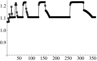
Having described how to determine conditions which guarantee existence of a reconstruction, in the next section we apply this approach to a number of example problems. First, however, it is instructive to confirm that these conditions do indeed guarantee stability of the recontruction procedure. In Figure 6 we plot ‖(ϵ​A^)−1‖\|(\epsilon\hat{A})^{-1}\| against nn (for ϵ=0.5\epsilon=0.5), where A^\hat{A} is formed via (4.19) using Haar wavelets with parameter m=⌈4.9​n⌉m=\lceil 4.9n\rceil. As we observe, the quantity remains bounded, indicating stability. Note the stark contrast to the severe instability documented in Figure 2.
Refer to caption
Figure 6: The quantity ‖(ϵ​A^)−1‖\|(\epsilon\hat{A})^{-1}\| against n=2,4,…,360n=2,4,\ldots,360.

6 Examples

In this final section, we consider the application of the generalized sampling theorem to several examples.

6.1 Reconstruction from the Fourier Transform

In this example we consider the following problem. Let f∈L2​(ℝ)f\in L^{2}(\mathbb{R}) be such that

f=ℱ​g,supp⁡(g)⊂[−T,T].f=\mathcal{F}g,\qquad\mathrm{supp}(g)\subset[-T,T].

We assume that we can access point samples of ff, however, it is not ff that is of interest to us, but rather gg. This is a common problem in applications, in particular MRI. The NS Sampling Theorem assures us that we can recover gg from point samples of ff as follows:

g=ϵ∑n=−∞∞f(nϵ)e2πinϵ⋅,ϵ=12​T,g=\epsilon\sum_{n=-\infty}^{\infty}f(n\epsilon)\,e^{2\pi\mathrm{i}n\epsilon\cdot},\qquad\epsilon=\frac{1}{2T},

where the series converges in L2L^{2} norm. Note that the speed of convergence depends on how well gg can be approximated by the functions e2πinϵ⋅e^{2\pi\mathrm{i}n\epsilon\cdot}, n∈ℤ.n\in\mathbb{Z}. Suppose now that we consider the function

g⁡(t)=cos⁡(2​π​t)​χ[0.5,1]​(t).g(t)=\cos(2\pi t)\chi_{[0.5,1]}(t).

In this case, due to the discontinuity, forming

gN=ϵ∑n=−NNf(nϵ)e2πinϵ⋅,ϵ=12,N∈ℕ,g_{N}=\epsilon\sum_{n=-N}^{N}f(n\epsilon)\,e^{2\pi\mathrm{i}n\epsilon\cdot},\qquad\epsilon=\frac{1}{2},\quad N\in\mathbb{N}, (6.1)

may be less than ideal, since the convergence gN→gg_{N}\rightarrow g as N→∞N\rightarrow\infty may be slow.

This is, of course, not an issue if we can access all the samples {f⁡(n​ϵ)}n∈ℤ,\{f(n\epsilon)\}_{n\in\mathbb{Z}}, however, such an assumption may be overly optimistic in application. Moreover, even if we had access to all samples, we are limited by both processing power and storage to taking only a finite number.

Refer to caption
Refer to caption
Refer to caption
Refer to caption
Refer to caption
Refer to caption
Figure 7: The upper figures show gNg_{N} (left), g~n,m\tilde{g}_{n,m} (middle) and gg (right) on the interval [0,1][0,1]. The lower figures show gNg_{N} (left), g~n,m\tilde{g}_{n,m} (middle) and gg (right) on the interval [0.47,0.57][0.47,0.57].

Suppose that we have a more realistic scenario: namely, we are given the finite collection of samples

ηf={f⁡(−N​ϵ),f⁡((−N+1)​ϵ),…,f⁡((N−1)​ϵ),f⁡(N​ϵ)},\eta_{f}=\{f(-N\epsilon),f((-N+1)\epsilon),\ldots,f((N-1)\epsilon),f(N\epsilon)\}, (6.2)

with N=900N=900 and ϵ=12.\epsilon=\frac{1}{2}. The task is now as follows: construct the best possible approximation to gg based on the vector ηf.\eta_{f}. We can naturally form gNg_{N} as in (6.1). This approximation can be visualized in the diagrams in Figure 7. Note the rather unpleasant Gibbs oscillations that occur, as discussed previously. The problem is simply that the set {e2πinϵ⋅}n∈ℤ\{e^{2\pi\mathrm{i}n\epsilon\cdot}\}_{n\in\mathbb{Z}} is not a good basis to express gg in. Another basis to use may be the Haar wavelets {ψj}\{\psi_{j}\} on [0,1][0,1] (we do not claim that this is the optimal basis, but at least one that may better capture the discontinuity of gg). In particular, we may express gg as

g=∑j=1∞βj​ψj,β={β1,β2,…}∈l2​(ℕ).g=\sum_{j=1}^{\infty}\beta_{j}\psi_{j},\qquad\beta=\{\beta_{1},\beta_{2},\ldots\}\in l^{2}(\mathbb{N}).

We will now use the technique suggested in Theorem 4.8 to construct a better approximation to gg based on exactly the same input information: namely, ηf\eta_{f} in (6.2). Let U^\widehat{U} be defined as in (4.18) with ϵ=1/2\epsilon=1/2 and let n=500n=500 and m=1801.m=1801. In this case

‖(PnU^∗PmU^Pn|Pn​ℋ)−1‖≤0.6169,‖(PnU^∗PmU^Pn|Pn​ℋ)−1PnU^∗Pm‖≤0.7854\begin{split}\left\|\left(P_{n}\widehat{U}^{*}P_{m}\widehat{U}P_{n}\lvert_{P_{n}\mathcal{H}}\right)^{-1}\right\|&\leq 0.6169,\\ \left\|\left(P_{n}\widehat{U}^{*}P_{m}\widehat{U}P_{n}\lvert_{P_{n}\mathcal{H}}\right)^{-1}P_{n}\widehat{U}^{*}P_{m}\right\|&\leq 0.7854\end{split}

Define β~={β~1,…,β~n}\tilde{\beta}=\{\tilde{\beta}_{1},\ldots,\tilde{\beta}_{n}\} by equation (4.19), and let g~n,m=∑j=1nβ~j​ψj.\tilde{g}_{n,m}=\sum_{j=1}^{n}\tilde{\beta}_{j}\psi_{j}. The function g~n,m\tilde{g}_{n,m} is visualized in Figure 7. Although, the construction of gNg_{N} and g~n,m\tilde{g}_{n,m} required exactly the same amount of samples of ff, it is clear from Figure 7 that g~n,m\tilde{g}_{n,m} is favorable. In particular, approximating gg by g~n,m\tilde{g}_{n,m} gives roughly four digits of accuracy. Moreover, had both nn and mm been increased, this value would have decreased. In contrast, the approximation gNg_{N} does not converge uniformly to gg on [0,1][0,1].

6.2 Reconstruction from Point Samples

In this example we consider the following problem. Let f∈L2​(ℝ)f\in L^{2}(\mathbb{R}) such that

f=ℱ​g,g⁡(x)=∑j=1Kαj​ψj​(x)+sin⁡(2​π​x)​χ[0.3,0.6]​(x),f=\mathcal{F}g,\qquad g(x)=\sum_{j=1}^{K}\alpha_{j}\psi_{j}(x)+\sin(2\pi x)\chi_{[0.3,0.6]}(x),

for K=400,K=400, where {ψj}\{\psi_{j}\} are Haar wavelets on [0,1],[0,1], and {αj}j=1K\{\alpha_{j}\}_{j=1}^{K} are some arbitrarily chosen real coefficients in [0,10][0,10]. A section of the graph of ff is displayed in Figure 8. The NS Sampling Theorem yields that

f⁡(t)=∑k=−∞∞f⁡(k2)​sinc​(2​t−k),f(t)=\sum_{k=-\infty}^{\infty}f\left(\frac{k}{2}\right)\mathrm{sinc}(2t-k),

where the series converges uniformly. Suppose that we can access the following pointwise samples of ff:

ηf={f⁡(−N​ϵ),f⁡((−N+1)​ϵ),…,f⁡((N−1)​ϵ),f⁡(N​ϵ)},\eta_{f}=\{f(-N\epsilon),f((-N+1)\epsilon),\ldots,f((N-1)\epsilon),f(N\epsilon)\},

with ϵ=12\epsilon=\frac{1}{2} and N=600.N=600. The task is to reconstruct an approximation to ff from the samples ηf\eta_{f} in the best possible way. We may of course form

fN​(t)=∑k=−NNf⁡(k2)​sinc​(2​t−k),N=600.f_{N}(t)=\sum_{k=-N}^{N}f\left(\frac{k}{2}\right)\mathrm{sinc}(2t-k),\qquad N=600.
Refer to caption
Refer to caption
Figure 8: The figure shows Re⁡(f)\mathrm{Re}(f) (left) and Im⁡(f)\mathrm{Im}(f) (right) on the interval [−5000,5000][-5000,5000].

However, as Figure 9 shows, this approximation is clearly less than ideal as f⁡(t)f(t) is approximated poorly for large tt. It is therefore tempting to try the reconstruction based on Theorem 4.8 and the Haar wavelets on [0,1][0,1] (one may of course try a different basis). In particular, let

f~=∑j=1nβ~j​ℱ​ψj,n=500,\tilde{f}=\sum_{j=1}^{n}\tilde{\beta}_{j}\mathcal{F}\psi_{j},\qquad n=500,

where

A^β~=PnU^∗Pmηf,A^=PnU^∗PmU^Pn|Pn​ℋ,\widehat{A}\tilde{\beta}=P_{n}\widehat{U}^{*}P_{m}\eta_{f},\qquad\widehat{A}=P_{n}\widehat{U}^{*}P_{m}\widehat{U}P_{n}\lvert_{P_{n}\mathcal{H}},

with m=2​N+1=1201m=2N+1=1201 and U^\widehat{U} is defined in (4.18) with ϵ=1/2\epsilon=1/2. A section of the errors |f−fN||f-f_{N}| and |f−f~||f-\tilde{f}| is shown in Figure 9. In this case we have

‖(PnU^∗PmU^Pn|Pn​ℋ)−1‖≤0.9022,‖(PnU^∗PmU^Pn|Pn​ℋ)−1PnU^∗Pm‖≤0.9498.\begin{split}\left\|\left(P_{n}\widehat{U}^{*}P_{m}\widehat{U}P_{n}\lvert_{P_{n}\mathcal{H}}\right)^{-1}\right\|&\leq 0.9022,\\ \left\|\left(P_{n}\widehat{U}^{*}P_{m}\widehat{U}P_{n}\lvert_{P_{n}\mathcal{H}}\right)^{-1}P_{n}\widehat{U}^{*}P_{m}\right\|&\leq 0.9498.\end{split}

In particular, the reconstruction f~\tilde{f} is very stable. Figure 9 displays how our alternative reconstruction is favorable especially for large tt. Note that with the same amount of sampling information the improvement is roughly by a factor of ten thousand.

Refer to caption
Refer to caption
Figure 9: The figure shows the error |f−fN||f-f_{N}| (left) and |f−f~||f-\tilde{f}| (right) on the interval [−5000,5000][-5000,5000].

7 Concluding Remarks

The framework presented in this paper has been studied via the examples of Haar wavelets and Legendre polynomials. Whilst the general theory is now well developed, there remain many questions to answer within these examples. In particular,

  • (i)

    What is the required scaling of mm (in comparison to nn) when the reconstruction basis consists of Legendre polynomials, and how well does the resulting method compare with more well-established approaches for overcoming the Gibbs phenomenon in Fourier series? Whilst there have been some previous investigations into this particular approach [16, 19], we feel that the framework presented in this paper, in particular the estimates proved in Theorem 4.1, are well suited for understanding this problem. We are currently investigating this possibility, and will present our results in a future paper.

  • (ii)

    Whilst Haar wavelets have formed been the principal example in this paper, there is no need to restrict to this case. Indeed, Theorem 5.1 provides a first insight into using more sophisticated wavelet bases for reconstruction. Haar wavelets are extremely simple to work with, however the use of other wavelets presents a number of issues. In particular, it is first necessary to devise a means to compute the entries of the matrix UU in a more general setting.

    In addition, within the case of the Haar wavelet, there remains at least one open problem. The computations in Section 5.1 suggest that n↦Φ⁡(U,n,θ)n\mapsto\Phi(U,n,\theta) is bounded by a linear function in this case, meaning that Theorem 5.1 is overly pessimistic. This must be proven. Moreover, it remains to be seen whether a similar phenomenon holds for other wavelet bases.

  • (iii)

    The theory in this paper has concentrated on linear reconstruction techniques with full sampling. A natural question is whether one can apply non-linear techniques from compressed sensing to allow for subsampling. Note that, due to the infinite dimensionality of the problems considered here, the standard finite-dimensional techniques are not sufficient.

8 Acknowledgments

The authors would like to thank Emmanuel Candès and Hans G. Feichtinger for valuable discussions and input.

References

  • [1] A. Aldroubi. Oblique projections in atomic spaces. Proc. Amer. Math. Soc., 124(7):2051–2060, 1996.
  • [2] A. Aldroubi and H. Feichtinger. Exact iterative reconstruction algorithm for multivariate irregularly sampled functions in spline-like spaces: the LpL^{p}-theory. Proc. Amer. Math. Soc., 126(9):2677–2686, 1998.
  • [3] A. Böttcher. Infinite matrices and projection methods. In Lectures on operator theory and its applications (Waterloo, ON, 1994), volume 3 of Fields Inst. Monogr., pages 1–72. Amer. Math. Soc., Providence, RI, 1996.
  • [4] E. J. Candès and D. L. Donoho. Recovering edges in ill-posed inverse problems: optimality of curvelet frames. Ann. Statist., 30(3):784–842, 2002.
  • [5] E. J. Candès and D. L. Donoho. New tight frames of curvelets and optimal representations of objects with piecewise C2C^{2} singularities. Comm. Pure Appl. Math., 57(2):219–266, 2004.
  • [6] Y. Eldar. Sampling with arbitrary sampling and reconstruction spaces and oblique dual frame vectors. Journal of Fourier Analysis and Applications, 9(1):77–96, 2003.
  • [7] Y. Eldar. Sampling without input constraints: Consistent reconstruction in arbitrary spaces. In A. I. Zayed and J. J. Benedetto, editors, Sampling, Wavelets and Tomography, pages 33–60. Boston, MA: Birkhäuser, 2004.
  • [8] Y. Eldar and T. Werther. General framework for consistent sampling in Hilbert spaces. Int. J. Wavelets Multiresolut. Inf. Process., 3(3):347, 2005.
  • [9] H. Feichtinger and I. Pesenson. Recovery of band-limited functions on manifolds by an iterative algorithm. In Wavelets, frames and operator theory, volume 345 of Contemp. Math., pages 137–152. Amer. Math. Soc., Providence, RI, 2004.
  • [10] H. G. Feichtinger and S. S. Pandey. Recovery of band-limited functions on locally compact abelian groups from irregular samples. Czechoslovak Math. J., 53(128)(2):249–264, 2003.
  • [11] K. Gröchenig, Z. Rzeszotnik, and T. Strohmer. Quantitative estimates for the finite section method. Integral Equations Operator Theory, to appear.
  • [12] R. Hagen, S. Roch, and B. Silbermann. C∗C^{*}-algebras and numerical analysis, volume 236 of Monographs and Textbooks in Pure and Applied Mathematics. Marcel Dekker Inc., New York, 2001.
  • [13] A. C. Hansen. On the approximation of spectra of linear operators on Hilbert spaces. J. Funct. Anal., 254(8):2092–2126, 2008.
  • [14] A. C. Hansen. On the solvability complexity index, the n-pseudospectrum and approximations of spectra of operators. J. Amer. Math. Soc., 24(1):81–124, 2011.
  • [15] E. Heinemeyer, M. Lindner, and R. Potthast. Convergence and numerics of a multisection method for scattering by three-dimensional rough surfaces. SIAM J. Numer. Anal., 46(4):1780–1798, 2008.
  • [16] T. Hrycak and K. Gröchenig. Pseudospectral Fourier reconstruction with the modified inverse polynomial reconstruction method. J. Comput. Phys., 229(3):933–946, 2010.
  • [17] A. Jerri. The Gibbs phenomenon in Fourier analysis, splines, and wavelet approximations. Springer, 1998.
  • [18] A. J. Jerri. The shannon sampling theorem: its various extensions and applications: A tutorial review. Proc. IEEE, 65:1565–1596, 1977.
  • [19] J.-H. Jung and B. D. Shizgal. Generalization of the inverse polynomial reconstruction method in the resolution of the Gibbs phenomenon. J. Comput. Appl. Math., 172(1):131–151, 2004.
  • [20] D. W. Kammler. A first course in Fourier analysis. Cambridge University Press, Cambridge, second edition, 2007.
  • [21] M. Lindner. Infinite matrices and their finite sections. Frontiers in Mathematics. Birkhäuser Verlag, Basel, 2006. An introduction to the limit operator method.
  • [22] S. Mallat. A wavelet tour of signal processing. Academic Press Inc., San Diego, CA, 1998.
  • [23] H. Nyquist. Certain topics in telegraph transmission theory. Trans. AIEE, 47:617–644, Apr. 1928.
  • [24] C. E. Shannon. A mathematical theory of communication. Bell System Tech. J., 27:379–423, 623–656, 1948.
  • [25] E. Tadmor. Filters, mollifiers and the computation of the Gibbs’ phenomenon. Acta Numerica, 16:305–378, 2007.
  • [26] M. Unser. Sampling–50 years after Shannon. Proc. IEEE, 88(4):569–587, 2000.
  • [27] M. Unser and A. Aldroubi. A general sampling theory for nonideal acquisition devices. IEEE Trans. Signal Process., 42(11):2915–2925, 1994.
  • [28] E. T. Whittaker. On the functions which are represented by the expansions of the interpolation theory. Proc. Royal Soc. Edinburgh, 35:181–194, 1915.