Partition Functions of Non-Abelian Quantum Hall States

Partition functions are best defined for the Hall geometry of an annulus (see Fig. 1(a)), to which we add a compact Euclidean time coordinate for the inverse temperature $\beta$. This space geometry allows for the measure of the Hall current and is equivalent to the bar geometry (corresponding to $R\to\infty$), while enjoying some special symmetries. The disk geometry (Fig. 1(b)), describing isolated Hall droplets, can be obtained from the annulus by shrinking the inner radius to zero.

As space-time manifold, the annulus at finite temperature has the topology: ${\cal M}=S^{1}\times S^{1}\times I$, where $I$ is the finite interval of the radial coordinate. The edge excitations live on the boundary $\partial{\cal M}$, corresponding to two copies of a space-time torus $S^{1}\times S^{1}$: they are chiral and anti-chiral waves on the outer $(R)$ and inner $(L)$ edges, respectively. This geometry is particularly convenient owing to the symmetry under modular transformations acting on the two periodic coordinates and basically exchanging the space and time periods. The partition functions should be invariant under this geometrical symmetry that actually implies several physical conditions on the spectrum of the theory [17]. For simplicity, we consider the case of no bulk excitations inside the annulus: later we shall see how to include them.

The (grand canonical) partition function on the annulus is defined by [14]:

where the trace is over the states of the Hilbert space, ${\cal K}$ is a normalization and $(\tau,\zeta)$ are complex numbers. The total Hamiltonian and spin are given by:

The energy on both $L$ and $R$ edges, $E=(v/R)(L_{0}-c/24)$, is proportional to the dilatation operator in the plane $L_{0}$, with eigenvalue the conformal dimension $h$; it also includes the Casimir energy proportional to the Virasoro central charge $c$ [14]. The real and imaginary parts of $\tau$ are respectively given by the “torsion” $\eta$ and the inverse temperature $\beta$ times the Fermi velocity $v$; the parameter $\zeta$ is proportional to the chemical potential $\mu$ and electric potential difference between the edges $V_{o}$:

Note that the charges $Q^{L}$ and $Q^{R}$ are defined in (2.1) in such a way to obtain the correct coupling to the electric potential in (2.2). In the following, we shall momentarily choose a symmetric Hamiltonian for the two edges by adjusting the velocities of propagation of excitations, $v_{L}/R_{L}=v_{R}/R_{R}$.

Most theories of edge excitations in the quantum Hall effect are rational conformal theories (RCFT) [14]: their Hilbert space is divided into a finite number of “sectors”, each one describing a basic quasiparticle, with rational charge and statistics, together with the addition of electrons; for example, in the Laughlin states with filling $\nu=1/p$, there are $p$ sectors, $\lambda=1,\dots,p$, and the associated charge is $Q=\lambda/p+\mathbb{Z}$. In mathematical terms, each sector provides a representation of the maximally-extended chiral symmetry algebra, which contains the Virasoro conformal algebra as a subalgebra.

The trace over the Hilbert space in (2.1) can be divided into sub-sums relative to pairs of sectors, left and right for the inner and outer edges; the sum of states in each sector give rise to a character $\theta_{\lambda}(\tau,\zeta)$ of the extended algebra [14]. As a result, the partition function reduces to the finite-dimensional sum:

In this equation, the bar denotes complex conjugation and the suffix $(c)$ is the charge conjugation $C$, acting by: $Q\to-Q$, $\theta\to\theta^{c}$. The inner (resp. outer) excitations are described by $\theta_{\lambda}$ (resp. $\theta_{\mu}^{c}$), according to the definition (2.1). The coefficients ${\cal N}_{\ \lambda,\mu}$ are positive integer numbers giving the multiplicities of sectors of excitations to be determined by imposing modular invariance and some physical requirements.

In the case of the Laughlin fluids, the RCFT is an extension of the affine $\widehat{U(1)}$ algebra of the chiral Luttinger liquid ($c=1$). The characters are given by theta functions with rational characteristics [15]:

Note that each term in the summation is a character of a $\widehat{U(1)}$ representation with charge $Q=\lambda/p+k$, i.e. describes the addition of $k$ electrons to the basic anyon. The Dedekind function $\eta(\tau)$ in the denominator describes particle-hole excitations and the non-analytic is as a measure factor; both terms are explained in [15].

Owing to scale invariance, the doubly-periodic geometry of the torus is specified by the modular parameter $\tau=\omega_{2}/\omega_{1}$, the ratio of the two periods (${\rm Im}\tau>0$). The same toroidal geometry can be described by different sets of coordinates respecting periodicity, that are related among themselves by integer linear transformations with unit determinant. The transformation of the modular parameter is:

Modular transformations belong to the infinite discrete group $\Gamma\equiv PSL(2,\mathbb{Z})=SL(2,\mathbb{Z})/\mathbb{Z}_{2}$ (the quotient is over the global sign of transformations) [14]. There are two generators, $T\ :\ \tau\to\tau+1$ and $S\ :\ \tau\to-1/\tau$, satisfying the relations $S^{2}=\left(ST\right)^{3}=C$, where $C$ is the charge conjugation matrix, $C^{2}=1$ [14].

The invariance of the partition function under modular transformations is therefore given by:

Let us briefly recall from [15] the physical conditions corresponding to these symmetries. The $S$ invariance amounts to a completeness condition for the spectrum of the RCFT: upon exchanging time and space, it roughly imposes that the set of states at a given time is the same as that ensuring time propagation [14]. The $S$ transformation acts by a unitary linear transformation in the finite basis of the characters (2.4):

($\varphi$ is an overall phase and $N=p$ for Laughlin states). The matrix $S_{ab}$ determines the fusion rules of the RCFT through the Verlinde formula [14]; moreover, the dimension $N$ of the matrix is equal to the Wen topological order of the Hall fluid [1].

The action of the $T^{2}$ transformation is,

namely it allows states with integer or half-integer spin on the whole system. These are electron-like excitations that carry the electric current in and out of the system: thus, anyon excitations present on both edges, should combine between them to form global fermionic states. Note that the presence of fermions in the QHE implies the weaker invariance under $T^{2}$ rather than $T$: actually, $S$ and $T^{2}$ generate a subgroup of the modular group, $\Gamma_{\theta}\subset\Gamma$ [14].

The partition function should also be invariant under the transformations of the $\zeta$ variable, $\zeta\to\zeta+1$ and $\zeta\to\zeta+\tau$, that can be geometrically interpreted as a coordinate on the torus. In physical terms, these correspond to conditions on the charge spectrum. The first one,

requires that excitations possess total integer charge, $Q^{L}+Q^{R}\in\mathbb{Z}$ (no quasiparticles are present in the bulk). Thus, fractionally charged excitations at one edge must pair with complementary ones on the other boundary. Consider, for example, a system at $\nu=1/3$ and add one electron to it: it can split into one pair of excitations with, $(Q^{L},Q^{R})=(1/3,2/3),(0,1),(2/3,1/3),(1,0)$. The different splittings are related one to another by tuning the electric potential $V_{o}$ in (2.2).

The potential at the edges can be varied by adding localized magnetic flux inside the annulus; the addition of one flux quantum leads to a symmetry of the spectrum, as first observed by Laughlin [1]. This is actually realized by the transformation $\zeta\to\zeta+\tau$, corresponding to $V_{o}\to V_{o}+1/R$ (in our notations $e=c=\hbar=1$) [15]. The corresponding invariance of the partition function is:

This transformation is called “spectral flow”, because it amounts to a drift of each state of the theory into another one.

In the case of the Laughlin theory, the $T^{2},S,U,V$ transformations of the characters $\theta_{\lambda}$ (2.5) are given by [15],

These formulas show that the generalized characters $\theta_{\lambda}$ carry a unitary representation of the modular group, which is projective for $\zeta\neq 0$ (the composition law is verified up to a phase).

Note that the charge transported between the two edges by adding one flux quantum in the center ($V$ transformation) is equal to the Hall conductivity: indeed, $\theta_{\lambda}(\zeta+\tau)\propto\theta_{\lambda+1}(\zeta)$ corresponds to $\nu=1/p$. This provides a method to determine the value of $\nu$ from the partition function.

The corresponding sums of right $\widehat{U(1)}$ representations are given by $\overline{\theta}^{c}_{\mu}$ carrying charge $Q^{R}=\mu/p+{\mathbb{Z}}$. Finally, the $U$ condition (2.10), applied to $Z_{\rm annulus}$ (2.4), requires that left and right charges obey: $\lambda+\mu=0$ mod $p$. This form of the partition function also satisfies the other conditions, $T^{2},S,V$, by unitarity.

Finally, the modular invariant partition function of Laughlin’s states is:

The partition function for the disk geometry is obtained from that of the annulus (2.13) by letting the inner radius to vanish, $R_{L}\to 0$ (see Fig. 1(b)). To this effect, the variable $\overline{\tau}$ in $\overline{\theta}_{\lambda}$ should be taken independent of $\tau$: ${\rm Im}\tau\neq-{\rm Im}\overline{\tau}$, $v_{R}/R_{R}\neq v_{L}/R_{L}$. The annulus partition function is no longer a real positive quantity but remains modular invariant, up to a global phase. In the limit $R_{L}\to 0$, the $\overline{\theta}_{\lambda}$ are dominated by their $|q|\to 0$ behavior: therefore, only the ground state sector remains in (2.13), leading to $\overline{\theta}_{\lambda}\to\delta_{\lambda,0}$, up to zero-point energy contributions. One finds: $Z_{\rm disk}^{(0)}=\theta_{0}$. In presence of quasiparticles in the bulk of the disk, with charge $Q_{\rm Bulk}=-a/q$, the condition of total integer charge selects another sector, leading to:

This is the desired result for the partition function on the disc geometry; there are $N$ such functions, $a=1,\dots,N$, that transforms unitarily among themselves under $S$ as a $N$-dimensional vector. Note here a manifestation of the general correspondence between bulk and edge excitations, that can be proven by using Chern-Simons theory but is actually valid for general RCFTs [29]: bulk excitations are equivalent, as much as the low-energy theory is concerned, to an edge with radius shrinking to zero; in this limit, the tower of excitations in that sector decouples.

The construction of RCFTs for quantum Hall states, both Abelian and non-Abelian, has been relying on a set of conditions for the spectrum of charge and statistics that implement the properties of electron excitations [18]; they should have:

A) integer charge;

B) Abelian fusion rules with all excitations;

C) fermionic statistics among themselves (half-integer spin);

D) integer statistics with all other excitations (integer exponent of mutual exchange).

The (B) and (D) conditions characterize the operator-product expansion of the conformal field $\Phi_{e}(z)$, representing the electron, with the field $\Phi_{i}(w)$ of a quasiparticle: for $z\to w$, this is,

The mutual statistics exponents is given by the conformal dimensions,

respectively of: the electron field, the $i$-th quasiparticle and their fusion product, $\Phi_{e\times i}=\Phi_{e}\times\Phi_{i}$. In general, excitations are made of a neutral part, described by a non-trivial RCFT, typically a coset theory $G/H$, and by a charged part (Luttinger liquid, i.e. a $\widehat{U(1)}$ RCFT) [14]: the fields in the above formulas are made of neutral and charged parts, and their dimensions $h$ have contributions from both of them. The requirement of integer statistics of the electron with all excitations, $h_{ei}\in\mathbb{Z}$, is motivated by the properties of many-body wave functions (describing, e.g. states with a quasiparticle of $i$-th type), that are described by correlators of the same RCFT for edge excitations. This bulk-edge correspondence follows again from the description of Hall fluids in terms of the Chern-Simons theory and is believed to be true for all rational CFTs [29].

The condition of Abelian fusion rules restricts to one the number of terms in the r.h.s. of the operator product expansion (2.15): indeed, if there were more terms, all the corresponding $h_{ei}$ exponents would need to be simultaneously integer, a condition generically impossible to achieve. Even if it were satisfied, this would lead to a degeneracy of $n$-electron wave functions and to a unacceptable degenerate ground state. Non-Abelian fusion rules and associated degeneracies (the quantum dimensions $d_{a}$) are possible for quasiparticles but not for electrons (within the RCFT description, at least [30]).

In the following, we show that the electron conditions (A)-(D) can be re-derived from the requirement of modular invariance of the partition function. We find that, upon choosing the RCFT for the neutral part of excitations and identifying the field representing the electron, the modular conditions are sufficient to self-consistently determine the charge and statistics spectrum, as well as the filling fraction¹¹ 1 And the spin parts, for non-polarized Hall fluids., without the need of additional physical hypotheses.

Let us compare (A)-(D) with the modular conditions introduced in the previous section for Laughlin states. The condition (A) is clearly the same as the $U$ modular invariance (2.10), whose solution is the extended character $\theta_{\lambda}$ (2.4), that resums electron excitations added to the $\lambda$ quasiparticle.

The condition (B) of Abelian fusion rules of the electron has a natural correspondent in RCFT, where a field with such property is called a “simple current” $J\ (\equiv\Phi_{e})$. The notion of simple current was introduced for orbifold theories and their modular invariant partition functions, as we now briefly recall [14][31].

The action of the simple current is indicated by $J\times\Phi_{i}=\Phi_{J(i)}(\equiv\Phi_{e\times i})$; it implies an Abelian discrete symmetry in the theory that is generated by $\exp(2i\pi Q_{J})$, with:

This charge is the exponent for the monodromy discussed in (2.16) and is conserved in the fusion rules. The fields $\Phi_{i}$ can be organized in orbits, each orbit containing the fields generated by the repeated fusion with the simple current. The simple current and its powers generate an Abelian group by fusion that is called the “center” ${\cal G}$ of the conformal field theory.

The modular invariant partition function can be obtained by the orbifold construction corresponding to modding out the symmetry associated to the simple current. The result has the general form [31]:

in this equation, $a$ labels the orbits, $i_{a}$ is a representative point on each orbit, and $|{\cal S}_{a}|$ is the order of the stabilizer ${\cal S}_{a}$ of the orbit $a$, i.e. the subgroup of ${\cal G}$ acting trivially on any element $i$ in $a$. The proof of the general expression (2.18) is not trivial and it involves the symmetry of the $S$ matrix under the $J$ action: $S_{i,J(k)}=S_{i,k}\exp(2i\pi Q_{J}(i))$. The modular invariants (2.18) can be considered as diagonal invariants with respect to the basis of the extended chiral algebra, whose characters are $\theta_{a}$. In the QHE case, the stabilizer is trivial and the $J$ action has no fixed points, owing to the additivity of the physical charge carried by the electron [32]. We recognize in (2.17),(2.18), the (D) condition (2.16) derived from QHE wave functions. Note that in the Abelian case this condition follows immediately from $U$ invariance [17].

Let us further analyze the solution (2.18); the $T^{2}$ invariance of the extended characters for the ground state and $a$-th quasiparticles, respectively $\theta_{0}$ and $\overline{\theta}_{a}$, implies:

The condition (C) of half-integer electron spin requires $M$ to be odd, i.e the even case is excluded for physical reasons (although sometimes allowed for bosonic fluids). Therefore, we should consider algebra extensions by half-integer spin currents, as in the case of the Neveu-Schwarz sector of supersymmetric theories [14]. (Note that the integer $N$ in (2.19) is also odd by the (D) condition).

In conclusion, we have re-derived the standard physical conditions (A)-(D) on Hall excitations from modular invariance of RCFT partition functions. They have been found to be diagonal invariants for extended symmetry algebras that are obtained in the orbifold construction through simple currents (in the present case without fixed points) [31].

In the following analysis of non-Abelian Hall fluids, we shall find that the (A)-(D) conditions (i.e. modular invariance) straightforwardly determine the charge and statistics spectrum of excitations, for a given choice of neutral RCFT and electron field (simple current). These results are relevant for model building: in the literature, the derivation of the theory pertaining to a given plateau often involves a combination of technical arguments and physical arguing, that might suggest a certain degree of arbitrariness in the construction of the theory, which is however not present.

We remark that the neutral RCFT may possess more than one simple current that could be used as electron field, although a preferred choice may exist, e.g. the lowest-dimensional field. This cannot be considered as an ambiguity of the construction, because the choice of electron field is part of the definition of the theory: different electrons correspond to different Hall states, with different charge spectra, filling fraction etc, all quantities being determined self-consistently.

Another possibility for RCFTs with two simple currents is that of using both of them simultaneously for building a modular invariant with further extended symmetry. This issue will be discussed in the conclusions.

In the following, the conditions (A)-(D) will be illustrated by rederiving the spectrum and partition functions [19] [17] of Read-Rezayi states [8] with filling fractions:

The Read-Rezayi theory is based on the neutral $\mathbb{Z}_{k}$ parafermion theory (${\rm PF}_{k}$) with central charge $c=2(k-1)/(k+2)$, that can be described by the standard coset construction ${\rm PF}_{k}=\widehat{SU(2)}_{k}/\widehat{U(1)}_{2k}$ [33]. Form the coset, we find that neutral sectors are characterized by a pair quantum numbers for the representations of the algebras in the numerator and denominator: these are $(\ell,m)$, equal to twice the $SU(2)$ spin and spin component, respectively ($m=\ell$ mod $2$).

The dimensions of parafermionic fields $\phi^{\ell}_{m}$ are given by:

The $\mathbb{Z}_{3}$ parafermion fields are shown in Fig. 2: the coset construction implies that the $m$ charge is defined modulo $2k$ [33]; indeed, the fields are repeated once outside the fundamental $(\ell,m)$ domain (2.21) by the reflection-translation, $(\ell,m)\to(k-\ell,m+k)$,

also called “field identification” [34].

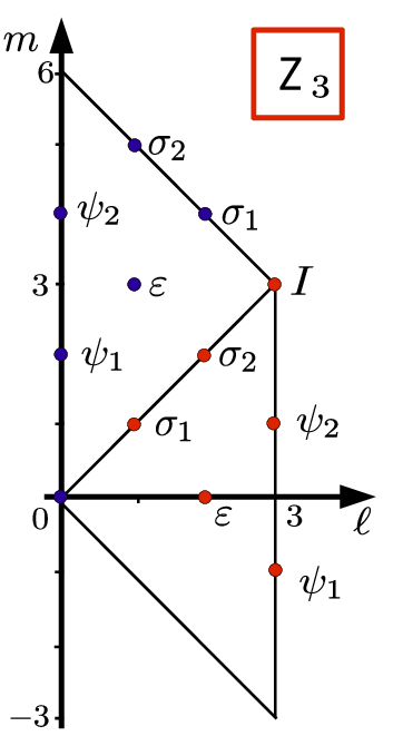
The fusion rules are given by the addition of the $\widehat{SU(2)}_{k}$ spin and $\widehat{U(1)}_{2k}$ charge:

The fields in the theory are called: parafermions, $\psi_{j}=\phi_{2j}^{0}$, $j=1,\dots,k-1$; spin fields, $\sigma_{i}=\phi_{i}^{i}$ ; and other fields. The parafermions have Abelian fusion rules with all the fields; among themselves, these are: $\psi_{i}\times\psi_{j}=\psi_{n}$, with $n=i+j$ mod $k$. The basic parafermion $\psi_{1}$ represents the neutral component of the electron in the Read-Rezayi states: the fusion $\left(\psi_{1}\right)^{k}=I$, describes the characteristic clustering of $k$ electrons in the ground state-wave function [8].

The excitations of the full theory are found by attaching $\widehat{U(1)}$ vertex operators to the parafermion fields: for the electron and a generic quasiparticle, we write,

with triplets of quantum numbers $(\alpha_{0},0,2)$ and $(\alpha,\ell,m)$, respectively. The mutual statistics exponent (2.16) is,

Upon substituting (2.21), the conditions (D) reads:

In particular, for the electron with itself, we find $\alpha_{0}^{2}-2/k=M$ integer; in combination with the condition (C) of half-integer electron spin,

it determines,

The electric charge $Q$ of excitations is proportional to the $\widehat{U(1)}$ charge, $Q=\mu\alpha$: the constant $\mu$ is fixed by assigning $Q=1$ to the electron, i.e. $\mu=1/\alpha_{0}$ ((A) condition).

In conclusion, the (A)-(D) conditions determine the charge and spin (i.e. half statistics) of excitations in the Read-Rezayi theory as follows:

The excitations are characterized by triplets of integer labels $(q,\ell,m)$, where $q$ is the charge index. From the Abelian part of conformal dimensions (2.30), we find that the Luttinger field is compactified into $p$ sectors (cf. (2.5)), $p=k(2+kM)$, and is indicated by $\widehat{U(1)}_{p}$; the charge index $q$ is thus defined modulo $p$. We write $p=k\hat{p}$, where $\hat{p}=2+kM$ is the denominator of the fractional charge; moreover, equation (2.29) shows that $q$ is coupled to the $SU(2)$ spin component $m$ by the selection rule:

We thus recover the $\mathbb{Z}_{k}$ “parity rule” of Ref. [19] that constraints charge and neutral quantum numbers of Read-Rezayi quasiparticle excitations. Earlier derivations of this rule were based on some physical conditions, such as a relation with a “parent Abelian state”, that were useful as motivations but actually not necessary (see, however, section 4.1.1). The present derivation shows that the relevant information is the type of RCFT for neutral excitations and the identification in this theory of the field $\psi_{1}$ representing the electron.

As outlined in the previous section, the derivation of annulus partition functions requires the solution of the modular invariance conditions: in particular, the $U$ symmetry (2.10) requires to put each basic anyon together with its electron excitations, leading to sectors of charge $Q=\lambda/p+\mathbb{Z}$ described by the RCFT extended character $\theta_{\lambda}$ as in (2.5). The addition of an electron changes the integer labels of excitations as follows:

Therefore, the extended characters $\theta_{\lambda}$ of the theory $PF_{k}\otimes\widehat{U(1)}_{p}$ are made of products of characters of the charged and neutral parts, whose indices obey the parity rule (2.31) and are summed over according to (2.32). The charged characters are given by the functions $K_{q}(\tau,k\zeta;k\hat{p})$ introduced earlier in (2.5), with parameters chosen to fit the fractional charge and the Abelian conformal dimension in (2.29). The $\mathbb{Z}_{k}$ parafermionic characters are denoted by $\chi^{\ell}_{m}(\tau;2k)$ and have rather involved expressions; actually it is enough to know their periodicities,

and modular transformation:

As recalled in Appendix A, this transformation can be obtained from the coset construction $PF_{k}=\widehat{SU(2)}_{k}/\widehat{U(1)}_{2k}$ [33].

The extended characters are thus given by products $K_{q}\chi^{\ell}_{m}$, with $q=m$ mod $k$ and $\ell=m$ mod $2$: adding one electron to the earlier product gives the term $K_{q+\hat{p}}\chi^{\ell}_{m+2}$; by continuing to add electrons until a periodicity is found, one obtain the expressions ²² 2 Hereafter, we disregard the non-analytic prefactor of $K$ for ease of presentation.,

that reproduce the charge and statistics spectrum (2.29), (2.30).

The expression (2.3) corresponds to the following solution of the parity rule (2.31):

(note $\hat{p}=2$ mod $k$). The other solution $m=k+a+2b$ mod $2k$ would lead to the same expressions with shifted index, $\theta^{k-\ell}_{a}$, owing to the field identification of parafermion fields $(\ell,m)\sim(k-\ell,m\pm k)$.

The $\theta_{a}^{\ell}$ characters have the periodicity, $\theta^{\ell}_{a+\hat{p}}=\theta^{k-\ell}_{a}$, that explains the ranges of indices indicated in (2.3); the dimension of the basis of $\theta^{\ell}_{a}$ characters is therefore given by $\hat{p}(k+1)/2$, in agreement with the value of the topological order of Read-Rezayi states [8] [19]. Moreover, the $V$ transformation of these characters reads, $\theta_{a}^{\ell}(\zeta+\tau)\sim\theta(\zeta)_{a+k}^{k-\ell}$, showing that the charge $\Delta Q=k/\hat{p}$ is created by adding one flux quantum: we thus recover the value of the filling fraction $\nu=k/(Mk+2)$ with $M$ odd.

The final step is to find the modular transformations of $\theta_{a}^{\ell}$, that is given by [17] (see Appendix A):

where the delta modulo two tells that $\theta^{\ell}_{a}(-1/\tau)$ vanishes for $a=\ell+1$ mod $2$ (we also disregard the global phase $\propto{\rm Re}(\zeta^{2}/\tau)$ acquired by the characters). In Appendix A, the check of the unitarity of the $S$ matrix confirms that the extended characters $\theta_{a}^{\ell}$ form an independent basis.

We remark that the coupling of neutral and charged parts by the $\mathbb{Z}_{k}$ parity rule and the sum over electron excitations amounts to a projection in the full $K_{\lambda}\chi^{\ell}_{m}$ tensor space to a subspace of dimension $1/k^{2}$ smaller: this reduction by a square factor is a standard property of $S$ transformations (i.e. discrete Fourier transforms). We also note that the $S$ matrix is factorized into charged and neutral parts, where the latter is the naive expression for the $\widehat{SU(2)}_{k}$ part, although the sectors are not factorized at all, as shown by the extended characters $\theta_{a}^{\ell}$.

Finally, the annulus partition function of Read-Rezayi states is given by the diagonal sesquilinear form,

that solves the $(S,T^{2},U,V)$ conditions of section 2.2.

For example, the expression of the $k=2$ Pfaffian state is as follows. The $\mathbb{Z}_{2}$ parafermions are the three fields of the Ising model: $\phi^{0}_{0}=\phi^{2}_{2}=I$, $\phi^{1}_{1}=\phi^{1}_{3}=\sigma$ and $\phi^{0}_{2}=\phi^{2}_{0}=\psi$, of dimensions $h=0,1/16,1/2$, respectively. For $\nu=5/2$, i.e. $M=1$ in (2.20), the Pfaffian theory possesses $6$ sectors. The partition function is:

where the neutral characters are written with the same symbol of the field and the charged ones are, $K_{\lambda}=K_{\lambda}(\tau,2\zeta;8)$, $K_{\lambda}=K_{\lambda+8}$, with charge $Q=\lambda/4+2\mathbb{Z}$. The first square term in $Z$ describes the ground state and its electron excitations, such as those in $K_{4}\psi$ with $Q=1+2\mathbb{Z}$; in the third and sixth terms, the characters $K_{\pm 1}\sigma$ contain the basic quasiparticles with charge, $Q=\pm 1/4$, and non-Abelian fusion rules $\sigma\cdot\sigma=I+\psi$. The other three sectors are less familiar: the second one contains a neutral Ising-fermion excitation (in $K_{0}\psi$) and the 4th and 5th sectors describe $Q=\pm 1/2$ Abelian quasiparticles.

As in section 2.1, the partition function on the disk is given by the extended character $\theta_{a}^{\ell}$, with indices selected by the quasiparticle type in the bulk; if there are many of them, their indices are combined by using the fusion rules to find the edge sector $(a,\ell)$.

In conclusion, the annulus and disk partition functions completely determine the Hilbert space of edge excitations and the fusion rules through the Verlinde formula. Physical applications to current experiments will be describe in section 4.

Some time ago, Block and Wen [13] considered the natural choice of RCFT with affine symmetry $\widehat{SU(m)}_{k}$ and the associated $SU(m)$ non-Abelian Chern-Simons theory, starting from the physical idea of breaking the electron excitation into $k$ fermions called “partons”. In such theories, there always are one or more simple currents. We shall limit ourselves to the simplest $SU(2)$ case, that has been recently considered in relation with the physics of second Landau level [3][25] and also serves as a starting point for other non-Abelian fluids.

We shall obtain the annulus partition function for the RCFT $\widehat{SU(2)}_{k}\otimes\widehat{U(1)}_{p}$. The $\widehat{SU(2)}_{k}$ theory is characterized by the primary fields $\phi^{\ell}$, for $\ell=0,1,\dots,k$, with dimensions $h_{\ell}=\ell(\ell+2)/(4(k+2))$. The simple current is $\phi^{k}$ with $h_{k}=k/4$ and fusion rules given by (cf. (2.23)):

which realizes a $\mathbb{Z}_{2}$ parity among the neutral sectors. Following the steps outlined in section 2.2, we introduce the fields $\Phi_{e}=\phi^{k}\exp(i\alpha_{0}\varphi)$, $\Phi_{i}=\phi^{\ell}\exp(i\alpha\varphi)$ corresponding to the electron and to a quasiparticle excitation, respectively.

The condition (D) on the mutual statistics exponent (2.16) of these excitations and of the electron with itself imply, respectively:

The charge and spin of excitations are therefore:

In particular, the condition (C) of half-integer electron spin requires that $(M+k)$ is odd.

The $\widehat{U(1)}_{p}$ contribution to the $J$ spectrum identifies the compactification parameter $p=2\hat{p}$, with $\hat{p}=(2M+k)$ the fractional-charge denominator. A quasiparticle is characterized by the integer pair $(\ell,2N+\ell)$ of $SU(2)$ spin and charge, that are constrained by the parity rule: $q=\ell$ mod $2$. The additions of one (two) electrons to a quasiparticle cause the following shifts (i.e. changes of sector):

that involves two non-Abelian sectors only.

Therefore, we are lead to consider extended characters $\theta^{\ell}_{a}$ of the full theory, labeled by spin $\ell$ and charge $a$ indices, that are made of products of charged characters, $K_{q}=K_{q}(\tau,2\zeta;2\hat{p})$ in the notation of (2.5), and $\widehat{SU(2)}_{k}$ characters $\chi^{\ell}(\tau)$, as follows:

Note that only two terms are needed in the sums, owing to the mentioned $\mathbb{Z}_{2}$ symmetry. As explained in section 2.2, the topological order of the $SU(2)$ NAF is given by the number of independent $\theta^{\ell}_{a}$ characters: the symmetry $\theta_{a+\hat{p}}^{k-\ell}=\theta_{a}^{\ell}$ confirms the index ranges indicated in (3.5). Furthermore, the filling fraction can be obtained from the $V$ transformation of $K_{a}$ characters: in summary, the $SU(2)$ NAF fluids are characterized by the values,

The modular transformations of extended characters can be obtained by those of the components $K_{a}$ and $\chi^{\ell}$ introduced in earlier sections: the result is (see Appendix A):

where $s_{\ell,\ell^{\prime}}$ is the $\widehat{SU(2)}_{k}$ $S$-matrix (2.34). The $S$-matrix of the full theory is again factorized in Abelian and non-Abelian parts (up to details) and is unitary.

In conclusion, the annulus partition function is given by the diagonal combination of extended characters,

with ranges of parameters given by (3.5). Each individual $\theta^{\ell}_{a}$ is the partition function on the disk geometry in presence of a specific bulk excitation.

It has been recently proposed [11] that a particle-hole conjugate of the $M=1$ Read-Rezayi fluids could be realizable in the second Landau level, with filling fractions $\nu-2=1-k/(k+2)=2/(k+2)$. In particular, for $\nu=5/2$ the Pfaffian state may compete with its conjugate state. The fluid of RR holes inside the $\nu=3$ droplet possesses an additional edge, leading to the CFT $\overline{SU(2)_{k}/U(1)_{2k}\otimes U(1)_{p}}\otimes\widehat{U(1)}$. The Luttinger liquids on edges of opposite chirality interact through impurities and re-equilibrate: the result of this process was shown to lead to the $\overline{SU(2)_{k}}\otimes\widehat{U(1)}_{p}$ edge theory [11] for the so-called anti-Read-Rezayi state ($\overline{\rm RR}$).

The partition function of this theory can be obtained as in the NAF case of the previous section, with little modifications due to the different chirality of the neutral sector. The electron and quasiparticle fields are given by $\Phi_{e}=\overline{\phi^{k}}\exp(i\alpha_{0}\varphi)$ and $\Phi_{i}=\overline{\phi^{\ell}}\exp(i\alpha\varphi)$, respectively (note that $\phi^{k}$ is the unique simple current of the $\widehat{SU(2)_{k}}$ theory).

In the mutual statistics exponent, the chiral and antichiral conformal dimensions should be subtracted leading to the conditions,

The charge and spin of excitations are therefore:

References

- [1] X. G. Wen, Quantum Field Theory of Many-body Systems, Oxford Univ. Press (2007), Oxford.
- [2] A. Stern, Anyons and the quantum Hall effect - a pedagogical review, Ann. Phys. 323 (2008) 204.
- [3] P. Bonderson, A. Kitaev, K. Shtengel, Detecting Non-Abelian Statistics in the Fractional Quantum Hall State , Phys. Rev. Lett. 96 (2006) 016803; W. Bishara, P. Bonderson, C. Nayak, K. Shtengel, J. K. Slingerland, Interferometric signature of non-Abelian anyons, Phys. Rev. B 80 (2009) 155303.
- [4] Y. Zhang, D. T. McClure, E. M. Levenson-Falk, C. M. Marcus, L. N. Pfeiffer, K. W. West, Distinct Signatures For Coulomb Blockade and Aharonov-Bohm Interference in Electronic Fabry-Perot Interferometers , Phys. Rev. B 79 (2009) 241304; R.L. Willett, L.N. Pfeiffer, K.W. West, Alternation and interchange of e/4 and e/2 period interference oscillations as evidence for filling factor 5/2 non-Abelian quasiparticles, preprint arXiv:0911.0345.
- [5] W. E. Chickering, J. P. Eisenstein, L. N. Pfeiffer, K. W. West, Thermopower of two-dimensional electrons at filling factors and , Phys. Rev. B 81 (2010) 245319.
- [6] G. Moore and N. Read, Nonabelions in the fractional quantum hall effect, Nucl. Phys. B 360 (1991) 362.
- [7] C. Nayak, S. H. Simon, A. Stern, M. Freedman, S. Das Sarma, Non-Abelian anyons and topological quantum computation, Rev. Mod. Phys. 80 (2008) 1083.
- [8] N. Read, E. Rezayi, Beyond paired quantum Hall states: Parafermions and incompressible states in the first excited Landau level, Phys. Rev. B 59 (1999) 8084.
- [9] E. Ardonne, K. Schoutens, New Class of Non-Abelian Spin-Singlet Quantum Hall States, Phys. Rev. Lett. 82 (1999) 5096; E. Ardonne, N. Read, E. Rezayi, K. Schoutens, Non-Abelian spin-singlet quantum Hall states: wave functions and quasihole state counting, Nucl. Phys. B 607 (2001) 549.
- [10] E. Ardonne, K. Schoutens, Wavefunctions for topological quantum registers, Annals Phys. 322 (2007) 201.
- [11] S.-S. Lee, S. Ryu, C. Nayak, M. P. A. Fisher, Particle-Hole Symmetry and the ν=5/2 Quantum Hall State, Phys. Rev. Lett. 99 (2007) 236807; M. Levin, B. I. Halperin, B. Rosenow, Particle-hole symmetry and the Pfaffian state, Phys. Rev. Lett. 99 (2007) 236806; W. Bishara, G. A. Fiete, C. Nayak. Quantum Hall states at : Analysis of the particle-hole conjugates of the general level- Read-Rezayi states, Phys. Rev. B 77 (2008) 241306.
- [12] P. Bonderson, J. K. Slingerland, Fractional Quantum Hall Hierarchy and the Second Landau Level, Annals Phys. 323 (2008) 2709.
- [13] B. Blok, X. G. Wen, Many body systems with non-Abelian statistics, Nucl. Phys. B 374 (1992) 615.
- [14] P. Di Francesco, P. Mathieu, D. Senechal, Conformal Field Theory, Springer (1999), Berlin.
- [15] A. Cappelli, G. R. Zemba, Modular invariant partition functions in the quantum Hall effect, Nucl. Phys. B 490 (1997) 595.
- [16] A. Cappelli, L. S. Georgiev, G. R. Zemba, Coulomb blockade in hierarchical quantum Hall droplets, J. Phys. A 42 (2009) 222001.
- [17] A. Cappelli, G. Viola, G. R. Zemba Chiral Partition Functions of Quantum Hall Droplets Ann. Phys, 325 (2010) 465.
- [18] N. Read, Excitation structure of the hierarchy scheme in the fractional quantum Hall effect, Phys. Rev. Lett. 65 (1990) 1502; J. Fröhlich, A. Zee, Large scale physics of the quantum hall fluid, Nucl. Phys. B 364 (1991) 517; X.-G. Wen, A. Zee, Classification of Abelian quantum Hall states and matrix formulation of topological fluids, Phys. Rev. B 46 (1992) 2290.
- [19] A. Cappelli, L. S. Georgiev, I. T. Todorov, Parafermion Hall states from coset projections of Abelian conformal theories, Nucl. Phys. B 599 (2001) 499.
- [20] R. Dijkgraaf, E. Verlinde, Modular invariance and the fusion algebra, Nucl. Phys. B (Proc. Suppl.) 5 B (1988) 87; G. Moore, N. Seiberg, Polynomial equations for rational conformal field theories, Phys. Lett. B 212 (1988) 451; Naturality in conformal field theory, Nucl. Phys. B 313 (1989) 16; for a review, see: Lectures on RCFT, proceedings of the 1989 Banff Summer school, H. C. Lee ed., Plenum Press (1990), New York.
- [21] A. Kitaev, J. Preskill, Topological Entanglement Entropy, Phys. Rev. Lett. 96 (2006) 110404; M. Levin, X.-G. Wen, Detecting Topological Order in a Ground State Wave Function, Phys. Rev. Lett. 96 (2006) 110405; O. S. Zozulya, M. Haque, K. Schoutens, E. H. Rezayi, Bipartite entanglement entropy in fractional quantum Hall states, Phys. Rev.B 76 (2007) 125310.
- [22] A. Stern, B. I. Halperin, Proposed Experiments to Probe the Non-Abelian Quantum Hall State, Phys. Rev. Lett. 96 (2006) 016802; R. Ilan, E. Grosfeld, A. Stern, Coulomb Blockade as a Probe for Non-Abelian Statistics in Read-Rezayi States, Phys. Rev. Lett. 100 (2008) 086803; R. Ilan, E. Grosfeld, K. Schoutens, A. Stern, Experimental signatures of non-Abelian statistics in clustered quantum Hall states, Phys. Rev. B 79 (2009) 245305.
- [23] A. Stern, B. Rosenow, R. Ilan, B. I. Halperin, Interference, Coulomb blockade, and the identification of non-abelian quantum Hall states, preprint arXiv:0912.4394; R. Ilan, B. Rosenow, A. Stern, Signatures of non-Abelian statistics in non-linear coulomb blockaded transport, preprint arXiv:1005.4772.
- [24] L. S. Georgiev, Thermal broadening of the Coulomb blockade peaks in quantum Hall interferometers, preprint arXiv:1003.4871.
- [25] P. Bonderson, C. Nayak, K. Shtengel, Coulomb Blockade Doppelgangers in Quantum Hall States, Phys. Rev. B 81 (2010) 165308.
- [26] N. R. Cooper, B. I. Halperin, I. M. Ruzin, Thermoelectric response of an interacting two-dimensional electron gas in a quantizing magnetic field, Phys. Rev. B 55 (1997) 2344.
- [27] N. R. Cooper, A. Stern, Observable Bulk Signatures of Non-Abelian Quantum Hall States, Phys. Rev. Lett. 102 (2009) 176807; K. Yang, B. I. Halperin, Thermopower as a possible probe of non-Abelian quasiparticle statistics in fractional quantum Hall liquids, Phys. Rev. B 79 (2009) 115317.
- [28] T. H. Hansson, C.-C. Chang, J. K. Jain, S. Viefers, Composite-fermion wave functions as correlators in conformal field theory, Phys. Rev. B 76 (2007) 075347; T. H. Hansson, M. Hermanns, S. Viefers, Quantum Hall quasi-electron operators in conformal field theory, Phys. Rev. B B 80 (2009) 165330; M. Hermanns, Condensing Non-Abelian Quasiparticles, Phys. Rev. Lett. 104 (2010) 056803.
- [29] E. Witten, Quantum field theory and the Jones polynomial, Commun. Math. Phys. 121 (1989) 351.
- [30] A. Cappelli, G. R. Zemba, Hamiltonian Formulation of the W-infinity Minimal Models, Nucl. Phys. B 540 (1999) 610.
- [31] J. Fuchs, A. N. Schellekens, C. Schweigert, A matrix S for all simple current extensions, Nucl. Phys. B 473 (1996) 323.
- [32] V.G. Kac, I.T. Todorov, Affine orbifolds and rational conformal field theory extensions of W-1+infinity, Commun. Math. Phys 190 (1997) 57.
- [33] A.B. Zamolodchikov, V.A. Fateev, Parafermionic Currents in the Two-Dimensional Conformal Quantum Field Theory and Selfdual Critical Points in Z(n) Invariant Statistical Systems, Sov. Phys. JETP 62 (1985) 215; D. Gepner, Z. Qiu, Modular invariant partition functions for parafermionic field theories, Nucl. Phys. B 285 (1987) 423. P. Jacob, P. Mathieu, Parafermionic character formulae, Nucl. Phys. B 587 (2000) 514.
- [34] D. Gepner, New Conformal Field Theories Associated with Lie Algebras and their Partition Functions, Nucl. Phys. B 290 (1987) 10; Field Identification In Coset Conformal Field Theories, Phys. Lett. B 222 (1989) 207.
- [35] J. K. Jain, Composite Fermions, Cambridge Univ. Press (2007), Cambridge.
- [36] A. Cappelli, C. A. Trugenberger, G. R. Zemba, Stable hierarchical quantum Hall fluids as minimal models, Nucl. Phys. B 448 (1995) 470; for a review, see: minimal models and the hierarchy of the quantum Hall effect, Nucl. Phys. (Proc. Suppl.) B 45A (1996) 112.
- [37] S. Hershfield, J. H. Davies, P Hyldgaard, C. J. Stanton, J. W. Wilkins, Zero-frequency current noise for the double-tunnel-junction Coulomb blockade, Phys. Rev. B 47 (1993) 1967; for a review, see: M.J.M. de Jong, C.W.J. Beenakker, Shot noise in mesoscopic systems,, in Mesoscopic Electron Transport, L.L. Sohn, L.P. Kouwenhoven, G. Schoen eds. (Kluwer, Dordrecht, 1997).
- [38] P. Fendley, M. P. A. Fisher, C. Nayak, Topological Entanglement Entropy from the Holographic Partition Function, J. Statist. Phys. 126 (2007) 1111; Boundary conformal field theory and tunneling of edge quasiparticles in non-Abelian topological states, Annals Phys. 324 (2009) 1547.
- [39] For a review, see: A. Cappelli, J. B. Zuber, A-D-E Classification of Conformal Field Theories, Scholarpedia 5 (2010) 10314.