A Fast Algorithm for Three-Dimensional Layers of Maxima Problem
Abstract
We show that the three-dimensional layers-of-maxima problem can be solved in time in the word RAM model. Our algorithm runs in deterministic time or expected time and uses space. We also describe a deterministic algorithm that uses optimal space and solves the three-dimensional layers-of-maxima problem in time in the pointer machine model.
1 Introduction
A point dominates a point if each coordinate of is larger than or equals to the corresponding coordinate of . A point is a maximum point in a set if no point of dominates . The maxima set of is the set of all maximum points in . In the layers-of-maxima problem we assign points of a set to layers , , according to the dominance relation: The first layer of is defined as the maxima set of , the layer of is the maxima set of , and the -th layer of is the maxima set of . In this paper we show that the three-dimensional layers-of-maxima problem can be solved in time.
Previous and Related Work. The algorithm of Kung, Luccio, and Preparata [23] finds the maxima set of a set in time for or dimensions and time for dimensions. The algorithm of Gabow, Bentley, and Tarjan [16] finds the maxima set in time for dimensions. Very recently, Chan, Larsen, and Pǎtraşcu [11] described a randomized algorithm that solves the -dimensional maxima problem (i.e., finds the maxima set) for in time. Numerous works are devoted to variants of the maxima problem in different computational models and settings: In [8], the authors describe a solution for the three-dimensional maxima problem in the cache-oblivious model. Output-sensitive algorithms and algorithms that find the maxima for a random set of points are described in [7, 13, 18, 22]. The two-dimensional problem of maintaining the maxima set under insertions and deletions is considered in [21]; the problem of maintaining the maxima set for moving points is considered in [15].
The general layers-of-maxima problem appears to be more difficult than the problem of finding the maxima set. The three-dimensional layers-of-maxima problem can be solved in time [1] using dynamic fractional cascading [24]. The algorithm of Buchsbaum and Goodrich [9] runs in time and uses space. Giyora and Kaplan [17] described a data structure for point location in a dynamic set of horizontal segments and showed how it can be combined with the approach of [9] to solve the three-dimensional layers-of-maxima problem in time and space.
The time is optimal even if we want to find the maxima set in two dimensions [23] provided that we work in the infinite-precision computation model in which input values, i.e. point coordinates, can be manipulated with algebraic operations and compared. On the other hand, it is well known that it is possible to achieve time (resp. time for searching in a data structure) for many one-dimensional as well as for some multi-dimensional problems and data structures in other computational models. For instance, the grid model, that assumes all coordinates to be integers in the range for a parameter , was extensively studied in computational geometry. Examples of problems that can be solved efficiently in the grid model are orthogonal range reporting queries [25] and point location queries in a two- and three-dimensional rectangular subdivisons [5]. In fact, we can use standard techniques to show that these queries can be answered in time when all coordinates are arbitrary integers. Recently, a number of other important geometric problems was shown to be solvable in time (resp. in time) in the word RAM model. An incomplete list11 1 We note that problems in this list are more difficult than the layers-of-maxima problem because in our case we process a set of axis-parallel segments. includes Voronoi diagrams and three-dimensional convex hulls in time [12], two-dimensional point location in time [26, 10], and dynamic convex hull in time [14]. Results for the word RAM model are important because they help us better understand the structure and relative complexity of different problems and demonstrate how geometric information can be analyzed in algorithmically useful ways.
Our Results. In this paper we show that the three-dimensional layers-of-maxima problem can be solved in deterministic time and space in the word RAM model. If randomization is allowed, our algorithm runs in expected time. For comparison, the fastest known deterministic linear space sorting algorithm runs in time [19]. Our result is valid in the word RAM computation model, but the time-consuming operations, such as multiplications, are only used during the pre-processing step when we sort points by coordinates (see section 2). For instance, if all points are on the grid, then our algorithm uses exactly the same model as [25] or [5].
We also describe an algorithm that uses space and solves the three-dimensional layers-of-maxima problem in optimal time in the pointer machine model [27]. The result of Giyora and Kaplan [17] that achieved the same space and time bounds is valid only in the RAM model. Thus we present the first algorithm that solves the three-dimensional layers-of-maxima problem in optimal time and space in the pointer machine model.
Overview. Our solution, as well as the previous results, is based on the sweep plane algorithm of [9] described in section 2. The sweep plane algorithm assigns points to layers by answering for each a point location query in a dynamically maintained staircase subdivision. We observe that general data structures for point location in a set of horizontal segments cannot be used to obtain an time solution. Even in the word RAM model, no dynamic data structure that supports both queries and updates in time is known. Moreover, by the lower bound of [2] any data structure for a dynamic set of horizontal segments needs time to answer a point location query. We achieve a significantly better result using the methods described below.
In section 3 we describe the data structure for point location in a staircase subdivision that supports queries in time and updates22 2 We will describe update operations supported by our data structure in sections 2 and 3. in poly-logarithmic time per segment. This result may be of interest on its own.
The data structure of section 3 is not sufficient to obtain the desired runtime and space usage mainly due to high costs of update operations. To reduce the update time and space usage, we construct auxiliary staircases , such that: 1. the total number of segments in and the total number of updates is for a parameter ; 2. locating a point among staircases gives us an approximate location of among the original staircases (up to staircases). An efficient method for maintaining staircases , described in section 4, is the most technically challenging part of our construction. In section 5 we show how the data structure of section 3 can be combined with the auxiliary staircases approach to obtain an time algorithm. We also sketch how the same approach enables us to obtain an time and space algorithm in the pointer machine model.
2 Sweep Plane Algorithm
Our algorithm is based on the three-dimensional sweep method that is also used in [9]. We move the plane parallel to the plane 33 3 We assume that all points have positive coordinates. from to and maintain the following invariant: when the -coordinate of the plane equals all points with are assigned to their layers of maxima. Here and further , , and denote the ,- -, and -coordinates of a point . Let be the set of points that belong to the -th layer of maxima such that ; let denote the projection of on the sweep plane, where denotes the projection of a point on the -plane. For each value of maximal points of form a staircase ; see Fig. 1. When the -coordinate of the sweep plane is changed from to , we assign all points with to their layers of maxima. If , such that , is dominated by a point from , then belongs to the -th layer of maxima and . If , such that , dominates a point on , then belongs to the -th layer of maxima and . We observe that dominates if and only if the staircase is dominated by , i.e., the vertical ray shot from in direction passes through . Hence, the point belongs to the layer , such that is between the staircase and the staircase . This means that we can assign a point to its layer by answering a point location query in a staircase subdivision. When all with are assigned to their layers, staircases are updated.
Thus to solve the layers of maxima problem, we examine points in the descending order of their -coordinates. For each , such that there is at least one with , we proceed as follows: for every with operation identifies the staircase immediately below . If the first staircase below has index ( may also lie on ), then is assigned to the -th layer of maxima; if is below the lowest staircase , then is assigned to the new layer . When all points with are assigned to their layers, the staircases are updated. All points such that are examined in the ascending order of their -coordinates. If a point with is assigned to layer , we perform operation that removes all points of dominated by and inserts into . If the staircase does not exist, then instead of we perform the operation ; creates a new staircase that consists of one horizontal segment with left endpoint and right endpoint and one vertical segment with upper endpoint and lower endpoint . See Fig. 1 for an example.
 |
 | |
| (a) | (b) |
We can reduce the general layers of maxima problem to the problem in the universe of size using the reduction to rank space technique [25, 16]. The rank of an element is defined as the number of elements in that are smaller than : ; clearly, . For a point , , let . Let . Coordinates of all points in belong to range . A point dominates a point if and only if , , and where , , are sets of -, -, and -coordinates of points in . Hence if a point is assigned to the -th layer of maxima of , then belongs to the -th layer of maxima of . We can find ranks of , , and coordinates of every point by sorting , , and . Using the sorting algorithm of [19], , , and can be sorted in time and space. Thus the layers of maxima problem can be reduced to the special case when all point coordinates are bounded by in time.
3 Fast Queries, Slow Updates
In this section we describe a data structure that supports in time and update operations and in time per segment. We will store horizontal segments of all staircases in a data structure that supports ray shooting queries: given a query point identify the first segment crossed by a vertical ray that is shot from in direction; in this case we will say that the segment precedes (or is the predecessor segment of ). In the rest of this paper, segments will denote horizontal segments. Identifying the segment that precedes is (almost) equivalent to answering a query . Operation corresponds to a deletion of all horizontal segments dominated by and an insertion of at most two horizontal segments, see Fig 1. Operation corresponds to an insertion of a new segment.
Our data structure is a binary tree on -coordinates and segments are stored in one-dimensional secondary structures in tree nodes. The main idea of our approach is to achieve fast query time by binary search of the root-to-leaf path: using properties of staircases, we can determine in time whether the predecessor segment of a point is stored in the ancestor of a node or in the descendant of a node for any node on the path from the root to . Our approach is similar to the data structure of [5], but we need additional techniques to support updates.
For a horizontal segment , we denote by and the -coordinates of its left and right endpoints respectively; we denote by the -coordinate of all points of . An integer precedes (follows) an integer in if is the largest (smallest) element in , such that (). Let be a set of segments and let be the set of -coordinates of segments in . We say that precedes (follows) an integer if the -coordinate of precedes (follows) in . Thus a segment that precedes a point is a segment that precedes in the set of all segments that intersect the vertical line .
We construct a balanced binary tree of height on the set of all possible -coordinates, i.e., leaves of correspond to integers in . The range of a node is the interval where and are leftmost and rightmost leaf descendants of .
We say that a segment spans a node if ; a segment belongs to a node if . A segment -cuts a node if intersects the vertical line , but does not span , i.e., and ; a segment -cuts a node if intersects the vertical line but does not span , i.e., and . A segment such that either cuts , or spans , or belongs to . We store -coordinates of all segments that -cut (-cut) a node in a data structure (). Using exponential trees [4], we can implement and in linear space, so that one-dimensional searching (i.e. predecessor and successor queries) is supported in time. Since a segment cuts nodes (at most two nodes on each tree level), all and use space. We denote by the index of the staircase that contains , i.e., . The following simple properties are important for the search procedure:
Fact 1
Suppose that an arbitrary vertical line cuts staircases and , , in points and respectively. Then because staircases do not cross.
Fact 2
For any two points and on a staircase , if , then
Fact 3
Given a staircase and a point , we can determine whether is below or above and find the segment such that in time. The data structure that supports such queries uses linear space and supports finger updates in time.
Proof
The data structure contains -coordinates of all segment endpoints of . is implemented as an exponential tree so that it uses space. Using we can identify such that in time; is below if and only if is below .
Using Fact 3
we can determine whether a segment precedes a point
in time: Suppose that belongs to a staircase
. Then is the predecessor segment of iff , and the
staircase is above .
We can use these properties and data structures
and to determine whether a segment that precedes
a point spans
a node , belongs to a node , or cuts a node . If the segment
we are looking for spans , then it cuts an ancestor of ; if that
segment belongs to , then it cuts a descendant of . Hence, we can
apply binary search and find in iterations the node
such that the predecessor segment of cuts .
Observe that in some situations there may be no staircase below
, see Fig 4 for an example. To deal with such situations, we insert
a dummy segment with left endpoint and right endpoint
; we set and store in the data structure
where is the root of .
Let be the leaf in which the predecessor of is stored. We will use variables , and to guide the search for the node . Initially we set and is the root of . We set to be the middle node between and : if the path between and consists of edges, then the path from to consists of edges and is an ancestor of .
Let and denote the segments in that precede and
follow .
If there is no segment in with , then
we set .
If there is no segment in with , then
we set .
We can find both and in time.
If the segment , we check whether the staircase
contains the predecessor segment of ; by Fact 3,
this can be done in time.
If contains the predecessor segment of ,
the search is completed.
Otherwise, the staircase is below or
.
In this case we find the segment that precedes in .
If is not the predecessor segment of or ,
then the predecessor segment of either spans or belongs to .
We distinguish between the following two cases:
1. The segment and the staircase that contains is
below . By Fact 1, a vertical line
will cross the staircase of before it will cross
a staircase , . Hence, a segment that spans and
belongs to the staircase , , cannot
be the predecessor segment of . If a segment spans and
, then the -coordinate of is larger than the
-coordinate of by Fact 1. Since and
,
the segment is above .
Thus no segment that spans can be the predecessor
of .
2. The staircase that contains is above or .
If exists, the staircase
is below . Hence, the predecessor segment of
belongs to a staircase44
4
To simplify the description,
we assume that if .
, .
Since each staircase , ,
contains a segment that spans , the predecessor segment of is
a segment that spans .
If does not exist, then every segment below the point spans
the node . Hence, the predecessor segment of spans .
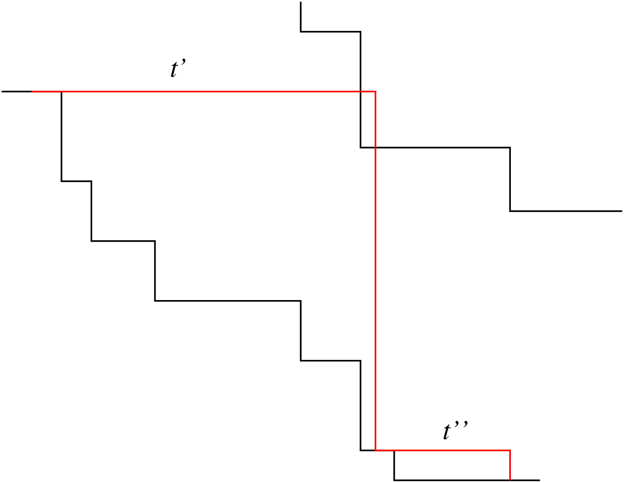
See Fig. 2 for an example.
 |
 |
 | |
| (a) | (b) | (c) |
If the predecessor segment spans , we search for among ancestors of ; if the predecessor segment belongs to , we search for among descendants of . Hence, we set in case 2, and we set in case 1. Then, we set to be the middle node between and and examine the new node . Since we examine nodes and spend time in each node, the total query time is .
If the predecessor segment is the dummy segment , then there is no horizontal segment of any below . In this case we must identify the staircase to the left of . Let denote the rightmost point on the staircase , i.e., is a point on such that . Then is between staircases and , such that . We can find in time.
When a segment is deleted, we delete it from the corresponding data structure . We also delete from all data structures and for all nodes and , such that -cuts (respectively -cuts ). Since a segment cuts nodes and exponential trees support updates in time, a deletion takes time. Insertions are supported in the same way55 5 The update time can be slightly improved using fractional cascading and similar techniques, but this is not necessary for our presentation.. Operation is implemented by inserting a segment with endpoints and into , incrementing by one the number of staircases , and creating the new data structure . To implement we delete the segments “covered” by from and and insert the new segment (or two new segments) into and .
Lemma 1
We can store horizontal staircase segments with endpoints on grid in a space data structure that answers ray shooting queries in time and supports operation in time where is the number of segments inserted into and deleted from the staircase , and operation in time.
The data structure of Lemma 1 is deterministic. We can further improve the query time if randomization is allowed.
Fact 4
Given a staircase and a point , we can determine whether is below or above and find the segment such that in time. The data structure that supports such queries uses linear space and supports finger updates in expected time.
Proof
Lemma 2
We can store horizontal staircase segments with endpoints on grid in a space data structure that answers ray shooting queries in time and supports operation in expected time where is the number of segments inserted into and deleted from the staircase , and operation in expected time.
Proof
Although this is not necessary for further presentation, we can prove a similar result for the case when all segment endpoints are on a grid; the query time is and the update time is per segment. See Appendix D for a proof of this result.
4 Additional Staircases
The algorithm in the previous section needs time to construct the layers of maxima: ray shooting queries can be performed in time, but update operations take time. To speed-up the algorithm and improve the space usage, we reduce the number of updates and the number of segments in the data structure of Lemma 1 to .
Let denote the data structure of Lemma 1. We
construct and maintain a new sequence of staircases
, where and the parameter will be
specified later. All horizontal segments of are stored
in . The new staircases satisfy the following conditions:
1. There are horizontal segments in all staircases
2. is updated times during the execution of the
sweep plane algorithm.
3. For any point and for any , if is between and
, then is situated between and
for .
Conditions 1 and 2 imply that the data structure uses space
and all updates of take time if .
Condition 3 means that we can
use staircases to guide the search among : we first identify
the index , such that the query point is between and
, and then locate in .
It is not difficult to construct that satisfy conditions 1 and 3.
The challenging part is maintaining the staircases with a small number
of updates.
Lemma 3
The total number of inserted and deleted segments in all is . The number of segments stored in is .
We describe how staircases can be maintained and prove Lemma 3 in Appendix B.
5 Efficient Algorithms for the Layers-of-Maxima Problem
Word RAM Model. To conclude the description of our main algorithm, we need the following simple
Lemma 4
Using a space data structure, we can locate a point in a group of staircases in time, where is the number of segments in . An operation is supported in time, where is the number of inserted and deleted segments in the staircase , .
Proof
We can use Fact 3 to determine whether a staircase is above or below a staircase for any . Hence, we can locate a point in time by a binary search among staircases.
We set . The data structure contains all segments of staircases for , where and is the highest index of a staircase; the data structure contains all segments of staircases . We can locate a point in each in time by Lemma 4. Since each staircase belongs to one data structure, all use space. We also maintain additional staircases as described in section 4. All segments of all staircases are stored in the data structure of Lemma 1; since contains segments, the space usage of is .
Now we can describe how operations , , can be implemented in time per segment.
- •
: We find the index , such that is between and in time. As described in section 4, is between and . Hence, we can use data structures , , and to identify such that is between and . Searching , , and takes time, and the total time for is .
- •
: let be the number of inserted and deleted segments. The data structure can be updated in time. We may also have to update , , and the data structure .
- •
: If for some , a new data structure is created. We add the horizontal segment of the new staircase into the data structure . If , we create a new staircase and add the segments of into the data structure .
There are update operations on the data structure that can be performed in time. If we ignore the time to update , then takes time and takes time. Since and is performed at most times, the algorithm runs in time. We thus obtain the main result of this paper.
Theorem 5.1
The three-dimensional layers-of-maxima problem can be solved in deterministic time in the word RAM model. The space usage of the algorithm is .
If we use Fact 4 instead of Fact 3 in the proof of Lemma 4 and Lemma 2 instead of Lemma 1 in the proof of Theorem 5.1, we obtain a slightly better randomized algorithm.
Theorem 5.2
The three-dimensional layers-of-maxima problem can be solved in expected time. The space usage of the algorithm is .
Pointer Machine Model. We can apply the idea of additional staircases to obtain an algorithm in the pointer machine model. This time, we set and maintain additional staircases as described in section 4. Horizontal segments of all are stored in the data structure of Giyora and Kaplan [17] that uses space and supports queries and updates in and time respectively, where is the number of segments in all and is an arbitrarily small positive constant. Using dynamic fractional cascading [24], we can implement so that uses linear space and answers queries in time. Updates are supported in time; details will be given in the full version of this paper. Using and , we can implement the sweep plane algorithm in the same way as described in the first part of this section. The space usage of all data structures is , and all updates of take time. By Lemma 3, the data structure is updated times; hence all updates of take time. The space usage of is . Each new point is located by answering one query to and at most three queries to ; hence, a new point is assigned to its layer of maxima in time.
Theorem 5.3
A three-dimensional layers-of-maxima problem can be solved in time in the pointer machine model. The space usage of the algorithm is .
Acknowledgment
The author wishes to thank an anonymous reviewer of this paper for a stimulating comment that helped to obtain the randomized version of the presented algorithm.
References
- [1] P.K. Agarwal. Personal communication.
- [2] S. Alstrup, T. Husfeldt, T Rauhe, Marked Ancestor Problems, Proc. FOCS 1998, 534-544.
- [3] M. J. Atallah, M. T. Goodrich, K. Ramaiyer, Biased Finger Trees and Three-dimensional Layers of Maxima, Proc. SoCG 1994, 150-159.
- [4] A. Andersson, M. Thorup, Dynamic Ordered Sets with Exponential Search Trees, J. ACM 54,Article No. 13 (2007).
- [5] M. de Berg, M. J. van Kreveld, J. Snoeyink, Two- and Three-Dimensional Point Location in Rectangular Subdivisions, J. Algorithms 18, 256-277 (1995).
- [6] M. A. Bender, R. Cole, E. D. Demaine, M. Farach-Colton, J. Zito, Two Simplified Algorithms for Maintaining Order in a List, Proc. ESA 2002, 152-164.
- [7] J. L. Bentley, K. L. Clarkson, and D. B. Levine, Fast Linear Expected-Time Algorithms for Computing Maxima and Convex Hulls, Proc. SODA 1990, 179-187.
- [8] G. S. Brodal, R. Fagerberg, Cache Oblivious Distribution Sweeping, Proc. ICALP 2002, 426-438.
- [9] A. L. Buchsbaum, M. T. Goodrich, Three-Dimensional Layers of Maxima, Algorithmica 39, 275-286 (2004).
- [10] T. M. Chan, Point Location in o(log n) Time, Voronoi Diagrams in o(n log n) Time, and Other Transdichotomous Results in Computational Geometry, Proc. FOCS 2006, 333-344.
- [11] T. M. Chan, K. Larsen, M. Pǎtraşcu, Orthogonal Range Searching on the RAM, Revisited, to be published in SoCG 2011.
- [12] T. M. Chan, M. Pǎtraşcu, Voronoi Diagrams in time, Proc. STOC 2007, 31-39.
- [13] K. L. Clarkson, More Output-Sensitive Geometric Algorithms, Proc. FOCS 1994, 695-702.
- [14] E. D. Demaine, M. Pǎtraşcu, Tight Bounds for Dynamic Convex Hull Queries (Again), Proc. SoCG 2007, 354-363.
- [15] P.G. Franciosa, C. Gaibisso, and M. Talamo, An Optimal Algorithm for the Maxima Set Problem for Data in Motion, Proc. CG 1992, 17-21.
- [16] H. N. Gabow, J. L. Bentley, R. E. Tarjan, Scaling and Related Techniques for Geometry Problems, Proc. STOC 1984, 135-143.
- [17] Y. Giyora, H. Kaplan, Optimal Dynamic Vertical Ray Shooting in Rectilinear Planar Subdivisions, ACM Transactions on Algorithms 5, (2009).
- [18] M. J. Golin, A Provably Fast Linear-Expected-Time Maxima-Finding Algorithm, Algorithmica 11, 501-524 (1994).
- [19] Y. Han, Deterministic Sorting in time and linear space. J. Algorithms 50, 96-105 (2004).
- [20] A. Itai, A. G. Konheim, M. Rodeh, A Sparse Table Implementation of Priority Queues, Proc. ICALP 1981, 417-431.
- [21] S. Kapoor, Dynamic Maintenance of Maximas of 2-d Point Sets, Proc. SoCG 1994, 140-149.
- [22] D. G. Kirkpatrick, R. Seidel,Output-Size Sensitive Algorithms for Finding Maximal Vectors, Proc. SoCG 1985, 89-96.
- [23] H. T. Kung, F. Luccio, F. P. Preparata, On Finding the Maxima of a Set of Vectors, J. ACM 22, 469-476 (1975).
- [24] K. Mehlhorn, S. Näher, Dynamic Fractional Cascading, Algorithmica 5, 215-241 (1990).
- [25] M. H. Overmars, Efficient Data Structures for Range Searching on a Grid, J. Algorithms 9(2), 254-275 (1988).
- [26] M. Pǎtraşcu, Planar Point Location in Sublogarithmic Time, Proc. FOCS 2006, 325-332.
- [27] R. E. Tarjan, A Class of Algorithms which Require Nonlinear Time to Maintain Disjoint Sets, J. Comput. Syst. Sci. 18(2), 110-127 (1979).
- [28] Dan E. Willard, Log-Logarithmic Worst-Case Range Queries are Possible in Space , Information Processing Letters 17(2), 81-84 (1983).
- [29] D. E. Willard, A Density Control Algorithm for Doing Insertions and Deletions in a Sequentially Ordered File in Good Worst-Case Time, Information and Computation 97, 150-204 (1992).
Appendix A. Figures


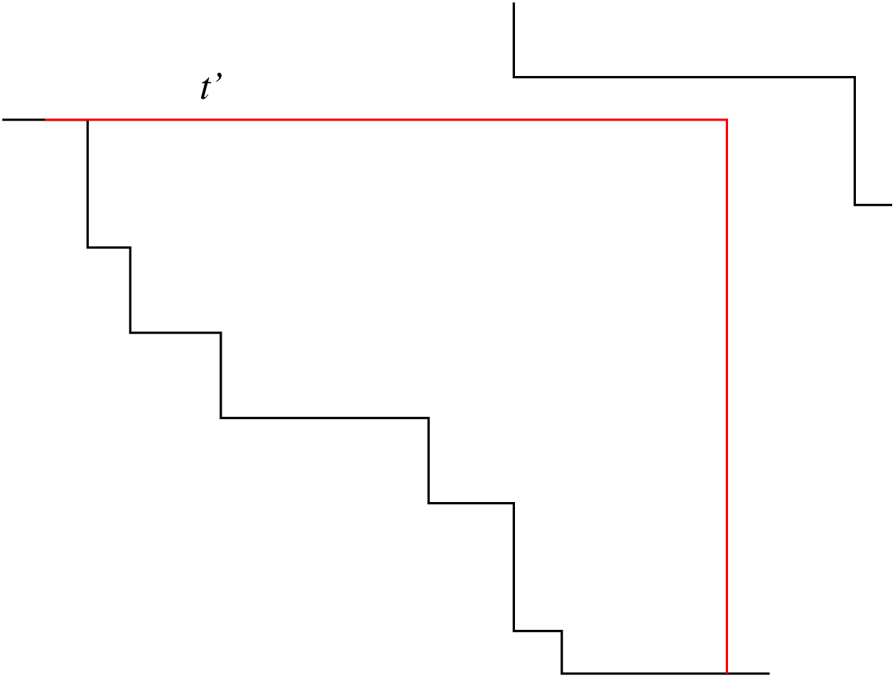
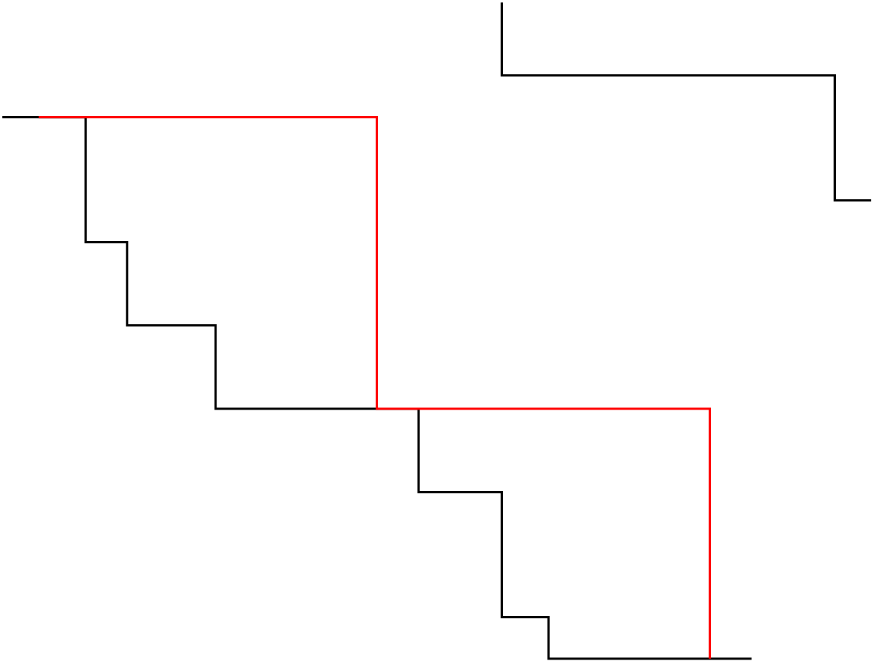 |
 | |
| (a) | (b) | |
 |
 | |
| (c) | (c) |
Appendix B. Proof of Lemma 3
In the first part of this section we describe the construction procedure of a boundary . Then, we will prove some facts about and describe the update procedure. In the last part of this section we will prove that all are updated times for updates of .
Construction of Additional Staircases. We construct one staircase for staircases . Let be the starting point of the staircase , i.e., and . The staircase is the path traced by as we alternatively move in the and direction until it hits the -axis.
A segment covers a point if . A segment is related to a segment if covers the left endpoint of ; a segment covers a segment if and . A point dominates a segment if dominates the left endpoint of . A segment follows the segment in a staircase or (resp. precedes s) if both and belong to the same staircase and .
Let . For convenience we assume that each point has
even -coordinate. This is achieved by replacing each point
with a point . Endpoints of all
segments of will have odd -coordinates.
The set contains all segments of
.
The staircase is constructed by repeating the following steps
until hits the -axis or the -coordinate of is maximal possible,
i.e. until or :
(1) We move in the direction until cuts ,
i.e until for a segment such that
(2) If , we move in direction until it hits
a segment of or .
Observe that at the beginning of step the point always belongs
to a horizontal segment of . Hence, a point on does
not dominate a segment of .
Since each horizontal segment
of cuts it also cuts , .
Hence, there are at least segments of related to each horizontal
segment of and the total number of segments in all
is .
An example of
a (just constructed) additional staircase is shown on
Fig. 3.
Updates.
When we update a staircase for
by operation , the
staircase is moved in the north-east direction. As a result,
a point on a staircase , , may dominate a segment
of . Therefore we maintain a weaker property:
no segment of
dominates and each point of is dominated by a
point on . Our goal is to update
times for updates of (in average).
We achieve this by maintaining the following invariants
Invariant 1
Each segment is dominated by the right endpoint of a segment .
Invariant 2
No point of is dominated by a point of .
Invariant 3
No segment cuts .
We say that a segment is empty if it does not cut .
Invariant 4
If a segment follows in , then either or is not empty.
If Invariants 1 and 3 are true when is constructed, they will not be violated after updates of . We update if Invariants 2 or 4 are violated: If a segment , such that was not empty when was inserted into , does not cut after an operation , we call the procedure that will be described later in this section. If a segment of is dominated by a point of after , we also call the procedure .
Fact 5
If a point dominates a segment of , then dominates at least one segment of for each .
Fact 6
If a point dominates more than two segments of , then dominates at least one segment of for each .
Proof
If dominates three segments of then dominates the right endpoint of at least one non-empty segment . Since cuts , the right endpoint of dominates a segment of . Hence, the right endpoint of dominates at least one segment of for by Fact 5. Since dominates the right endpoint of , also dominates at least one segment of for each .
Fact 7
Any point on , , dominates at most two segments of .
Proof
Suppose that a point on dominates more than two segments of . Then, there is a point on that also dominates more than two segments of . By Fact 6, dominates a segment of for each . Since a point on cannot dominate a point on , we obtain a contradiction.
Fact 7, which is a corollary of Invariant 4, guarantees us that each operation such that dominates affects at most two segments of . This will be important in our analysis of the number of updates of . Now we are ready to describe the update procedure.
The procedure deletes a segment and a number of preceding and following segments and replaces them with new segments. We say that a segment is the child of if was removed by an operation , such that is the right endpoint of ; is a descendant of if is a child of or a descendant of a child of . Let be the segment that precedes in . Let be segments of such that follows and follows for . Suppose that contained the right endpoint of a segment that belonged to when was inserted into , and let be the descendant of that belongs to when the procedure is performed. By Fact 7, may dominate the segment that precedes in , but does not dominate the segment that precedes in . Let be a descendant of a segment related to with the largest -coordinate of its right endpoint. By Fact 7, may dominate and but it cannot dominate .
Now we must decide which segments are to be deleted from and how to construct new segments. We delete segments that are dominated by or . As shown above, there are at most three such segments (except of itself). If , , is the last segment dominated by , we may also remove some segments that follow . But our guarantee is that all removed segments do not cut . We insert new segments into by moving a point in and directions. A more detailed description follows.
To simplify the description, we will use set
that contains some horizontal
segments that currently belong to and some segments
that belonged to but are already deleted.
When a staircase is constructed, contains all
horizontal segments of . When the procedure
is called, we delete all segments of dominated by or
and insert all segments , such that
. Segments
of are used to “bound the staircase from below”,
i.e. the left endpoint of each horizontal segment in belongs
to a segment from .
(1)
Let be the point on such that . This is the left
endpoint of the first inserted segment of .
(2) We move in the direction until or
cuts . While , we repeat the following
steps: we move in the direction until it hits “new”
; then, we move in direction until it
cuts . Observe that all horizontal segments inserted in step 2
cut .
(3) When , we move in direction until
it cuts and .
Suppose
that now for some in .
We continue
moving in direction until or cuts
. Then, we move in direction until hits
(4) We insert a new segment instead of the segment . It is possible
that now .
We move in direction until and move in
direction until hits .
(5) Now we must pay attention that Invariant 4 is
maintained: all inserted segments except of may be the last one are not
empty.
Let denote the last inserted segment, and suppose that both
and are empty. We can replace two empty segments
either with one empty segment, or one non-empty and one empty segment
as follows. We replace with a new segment :
the left endpoint of coincides with the left endpoint of and
either or
cuts .
If cuts , we replace with a new
segment such that , ,
and . See Fig. 5 for an example of
step (5).
Observe that all but one non-empty segments constructed by
cut . The only exception is the segment
constructed in step (3) that cuts .
We prove in Appendix C
that the total number of updates of
during the execution of the sweep plane algorithm is .
This completes the Proof of Lemma 3.
Appendix C. Analysis of Update Operations for Additional Staircases
We will show below that the data structure is updated times during the execution of the sweep-plane algorithm. First, we will estimate the number of deleted segments. We will estimate the number of insertions in the end of this section. We assign credit points to each segment of and credit points to every segment of for and . Insertion of a new segment into is free and deletion costs credit points.
Every time when we perform operation for we distribute the credit points of the newly inserted segment with right endpoint among several segments of . We evenly distribute credits of among segments such that either dominates or and where denotes the segment that follows in . By Fact 6 there are at most three such segments ; hence each obtains at least credits. When a segment of , , is deleted, we assign credits of to , such that is related to . We say that a segment is initially non-empty if cuts when is inserted into . We will show below that we can pay credit points for each deleted segment of and maintain the following property.
Property 1
Every initially non-empty segment
that does not cut , ,
accumulated at least credit points.
Every segment that is dominated by a point on
accumulated credit points.
Proof
Property 1 is obviously true for a just constructed staircase . Suppose that Property 1 is true after the procedure was called for segments of times. We will show that this property is maintained after the -th call of the procedure . If an initially non-empty segment does not cut after the -th call of is completed, then accumulated credits. If the segment does not cut at some point after the -th call of , then at least segments of , , that are related to are already deleted. Hence, accumulated at least credits. Therefore if an initially non-empty segment does not cut , then accumulated credits.
If a point of dominates a segment when the -th call of the procedure is completed, then has credit points. If a point of dominates a segment , then we performed at least one operation such that dominates for each . Hence, accumulated credits. Therefore if a segment of is dominated by a point on , then has credits.
Hence, when we start the procedure , the segment has credit points. In addition to , we may have to remove segments because a descendant of some segment , such that was related to when was constructed, dominates , , or . If segments are removed by , then each non-empty segment among does not cut . By Property 1, every such segment has credits. Since there are at least non-empty segments among , we can use credits accumulated by non-empty segments to remove . We use credits accumulated by to remove and to remove ,,,, and if necessary. If a segment inserted after the procedure cuts only staircases , then we transfer to the remaining credit points accumulated by . Recall that there is at most one such segment that may be inserted during step (3) of the update procedure. Since accumulated at least credit points and at most are spent for removing the segments , , , and , the segment obtains at least credit points after the update procedure.
We must also take care of the segment resp. segments and . Since it is possible that , can be dominated by a point of for some when it is constructed. Remaining credit points of segment are transferred to (resp. to ); if is constructed, then credit points of are transferred to . If is constructed but is not constructed (i.e. if replaces both and ), then credits of are also transferred to . If is dominated by a point of for some , then we performed an operation for each , such that and . Since and , was assigned credits for each . Hence, if is dominated by , then has at least credit points. The same is also true for and .
We can conclude from Property 1 that we can always pay credit points for a deleted segment of ; hence, the total number of deleted segments is .
Let be the number of segments in all when the algorithm is finished. Since for every second segment in there are at least segments of related to , the total number of segments in is where denotes the total number of segments in . Hence, . Clearly where is the number of inserted segments and is the number of deleted segments. Hence, and the total number of inserted and deleted segments in all is .
Appendix D. Staircases on Grid
Lemma 5
We can store horizontal staircase segments with endpoints on grid in a space data structure that answers ray shooting queries in time and supports operation in time where is the number of segments inserted into and deleted from the staircase , and operation in time.
Proof
Instead of storing point coordinates of segment endpoints in the data structure, we store labels of point coordinates: each and -coordinate is assigned an -label (-label), so that the -label (-label) of is smaller than the -label (-label) of if and only if (). All labels belong to range and are maintained using the technique of [20, 29]. When a new segment is inserted or deleted, labels may change, and we have to delete and re-insert into data structures those segments whose labels are changed. Since each segment is stored in secondary data structures, a deleted/inserted segment leads to updates in and . Hence the update time is . The query procedure is exactly the same as in the proof of Lemma 1.