Thermal behavior of charged dilatonic black branes in AdS
and
UV completions of Lifshitz-like geometries
Gaetano Bertoldi, Benjamin A. Burrington and Amanda W. Peet
†Department of Physics,
University of Toronto,
Toronto, Ontario, Canada M5S 1A7.
Several classes of gravitational backgrounds in dimensions have been proposed as holographic duals to Lifshitz-like theories describing critical phenomena in dimensions with critical exponent . We numerically explore one such model, characterized by a temperature and chemical potential , and find how to embed these solutions into AdS for a range of values of . We find no phase transition going from the to the regimes, and find that the solutions smoothly interpolate between the Lifshitz-like behavior and the relativistic AdS-like behavior. Finally, we exploit some conserved quantities to find a relationship between the energy density , entropy density , and number density , . We show that this result is expected from general scaling arguments, and generalizes to for a theory dual to AdSd+2 (Poincaré patch) asymptotics with a local gauge invariance.
1 Introduction
Since the Maldacena conjecture [1], AdS/CFT has become an important tool used to study non perturbative aspects of field theories (for a review see [2]). Traditionally, this has been used to study superconformal field theories in a particle physics context [3], however considerably less symmetric theories can be studied using holographic techniques [4]. It has also been fruitful to study toy models [5] that imitate certain features of string theory backgrounds, and seem to contain much of the physics11 1 Of course one always prefers string theory models where one can directly state what the weak coupling degrees of freedom are..
From the dimensional cases, it has been learned that finite temperature corresponds to the presence of a horizon in the gravitational dual. Further, gauge symmetries in the bulk correspond to conserved number operators in the dual field theory. Therefore, to study a field theory at finite temperature and chemical potential in a holographic setup, one studies charged objects with horizons in the bulk: charged black holes [6].
Holographic techniques have recently been applied to lower dimensional non-relativistic systems as well [7, 8, 9] (for reviews see [10]). In particular, much effort has gone into describing quantum critical behavior of these theories. Quantum critical systems exhibit a scaling symmetry
| (1) |
similar to the scaling invariance of pure AdS () in the Poincaré patch. From a holographic standpoint, this suggests the form of the spacetime metric
| (2) |
where the above scaling is realized as an isometry of the metric along with 22 2 Earlier studies of these metrics in a “brane world” scenario appear in [11]. It is also interesting to note that this metric, as well as several other “non-relativistic” metrics, are coset spaces [12].. The above metric has no symmetry that mixes time and space, although there are also models that contain a Galilean (or other non-relativistic) symmetry [8, 13, 14]. However, here we will be concerned with models that admit the metric (2) as a solution.
Often, a good place to begin studying any system is to write down a toy or “phenomenological” model [7, 8] to study generic properties. One may then consider possible embeddings into a more fundamental theory [13, 15, 16, 17], such as a string theory, where more information is known about the weakly coupled physics. Two toy models that admit the metric (2) have Lagrangians given by [18]
| (3) |
(we call this model for short) and [19]
| (4) |
(we call this model for short) where in either case is a two form field strength. There are also examples of actions with corrections that admit solutions of the form (2) [20].
There are several differences between the above models. First, the Lifshitz solution to model is truly invariant under the Lifshitz rescaling symmetry, while the solution with metric (2) of model has a logarithmically running dilaton, and so we call this a “Lifshitz-like” geometry. Note also that has a gauge symmetry while does not, and so the field theory dual to has a conserved particle number with chemical potential . Also of note is that model admits an exact black brane solution [19] that asymptotes to the metric (2), which can also be generalized to higher dimensions [21]. Finding black brane solutions for action has proven more difficult, and one often needs to resort to numeric methods [22, 23, 24], but not always [25] (an analogous analytic statement for an extension may be found in [26], and one should also see [27] where a certain extension to this model admits an analytic black hole). For extensions and variations to the basic model , see [26, 28], and for the holographically renormalized action, see [29].
In our current work we study the action , also studied in [19, 30, 31] (for variations and extensions, see [21, 32, 33, 34, 35, 36, 37]). In the Lifshitz-like solutions, the gauge field, and in fact the term in the Lagrangian, diverges. One immediately suspects that one must add a counter term on the boundary of the form , and one would expect this to change the ensemble from a fixed potential to a fixed charge (again, fixed in the boundary theory). One can also consider a fixed charge ensemble to simply be a limit where the chemical potential is large compared to other scales in the theory. Indeed, this is realized holographically by a geometry that interpolates between the Lifshitz-like solution and AdS; the large limit corresponds to a limit that leaves only the Lifshitz-like geometry.
We now consider such a solution. We take that the full geometry is the Lifshitz-like geometry in the limit, and is AdS for . This type of solution was already numerically studied in [31], and is essentially a relativistic (actually conformally invariant) UV completion of the theory. In the AdS asymptotics goes to a constant and goes to a constant, and so the growth in both and is cut off in this background. The size of is essentially cut off by the scale where the theory becomes like AdS. Conversely, the scale in the geometry is determined by , and we regard this as the chemical potential (where is the radius of AdS). Therefore, for such a geometry, we expect to have two regimes for energy scales: and . For the regime , the quantity provides a cutoff for new physics, i.e. it is the scale at which one can excite quanta associated with the conserved particle number, and can be considered the scale leading to the RG flow of in the Lifshitz-like background. Further we can see that if we perform the rescaling for large , we are zooming in on the Lifshitz-like part, and this is scaling . Combined with a time rescaling, this limit will eventually leave only the Lifshitz-like geometry.
There is of course another natural energy scale that one can introduce: the temperature . From the above, we expect there to be two regimes and , and we would like to know how the theory interpolates between these two known asymptotic solutions. We were initially motivated to find a possible phase transition when going from one regime to the other, as offers a new scale. Black hole phase transitions are typically first order; there are two solutions for a given set of boundary conditions, but each solution has different energy densities. Hence, during the phase transition, one expects a non homogeneous phase (when considering a fixed energy ensemble). However, we find no such phase transition when studying the system numerically. A possible explanation is that we are studying the vacua of a dimensional theory. As the vacua are time independent, the space of vacua for the theory are defined by a dimensional field theory. Such a field theory cannot have a phase transition that breaks the global translational and rotational symmetries (the inhomogeneous phase mentioned above) due to the ColemanMerminWagner (CMW) theorem (for a recent holographic study, see [38]). Therefore, one might expect no phase transition to occur (this leaves open the possibility that for greater values of the spatial dimension the theory might have different thermodynamic behavior). In all our results, we find a smooth, monotonic change in behavior from Lifshitz-like behavior to AdS-like behavior, similar to the “extremal” case studied numerically in [31].
We also explore the consequences of having certain conserved quantities along the flow, much in the same spirit as our earlier work [24, 25]. Using these conserved quantities, we are able to show that the energy density satisfies
| (5) |
where is the entropy density, and is the number density in the dual theory. We argue that this relation is actually expected in AdS. Essentially, the above relation along with the first law of thermodynamics allows one to write a pair of first order linear PDEs for and . The solutions to these differential equations have a scaling symmetry that reproduces the expected scaling dependence of AdS. In fact, the scaling dependence of AdS is shown to be equivalent to relation (5). This argument generalize to
| (6) |
in spatial dimensions (of the field theory), i.e. for a theory with AdSd+2 asymptotics and a local gauge theory in the bulk. We believe these arguments to be general enough to apply to any theory with only two scales and that has a conformally invariant UV fixed point.
We present this work as follows: in section 2 we perform a reduction of the action along a certain Ansatz and reproduce the equations of motion from this action. We find that the system reduces to 4 first order ODEs after introducing certain first integrals (conserved quantities), and further comment on the normalization of one such quantity, . We then perform a perturbative analysis of solutions near a regular horizon, around the AdS asymptotics, and around the Lifshitz-like solution, and display the exact AdS and Lifshitz black branes. We then discuss the setup for the numeric integration, and comment on how to read the chemical potential from the background. Finally, in section 3, we present the results of our numeric analysis, and the analysis that leads to equation (6).
2 Analysis of the model
2.1 Reduction
We wish to consider dilatonic black brane solutions to the equations of motion following from the action
| (7) |
We reduce the above action on the following Ansatz
| (8) |
where . We will get only ordinary differential equations in what follows, and so we define . We may reduce the action to a one dimensional action 33 3 we keep track of normalization for later use
| (9) |
with lagrangian
| (10) |
It can be verified that all equations of motion associated with the action (7) are reproduced by (10) as long as one uses the equation of motion for . Here, acts as a Lagrange multiplier, imposing the “zero energy” condition. Further, we note that allows for generic diffeomorphisms. We will refer to changing coordinate as “coordinate gauge” transformations, to differentiate from the gauge transformations associated with .
There are many conserved quantities associated with the above action. First, there is the conserved quantity associated with the shift symmetry . This can be understood as a rescaling of the time coordinate, and the coordinates that leaves invariant, and this then descends to the 1D action as Noether symmetry. Further, we note that there is the conserved quantity associated with which is exactly the gauge symmetry associated with . Further, we note that is also a symmetry. One can view this as saying that the dilaton here is exactly a space dependent gauge coupling, and we may absorb a normalization of the gauge coupling into the definition of . In addition, we have the Hamiltonian constraint as always. Now we count dynamical fields, and conserved quantities! This implies that the system is completely equivalent to a set of first order differential equations
| (11) | |||
| (12) | |||
| (13) | |||
| (14) |
Note, we still have not fixed a particular coordinate or gauge. While there are many conserved quantities above, one can see that they do not Poisson commute, and so the above is not an integrable system.
Now, let us simplify things a bit, and replace by using the last of the above relationships. We further take a different linear combination of the above equations, and find
| (15) | |||
| (16) | |||
| (17) | |||
| (18) |
where we have redefined the integration constants , for convenience. We note that is the only gauge dependent quantity, i.e. it transforms under the map , while the other equations do not. In the above, we have used the notation for a non normalized charge density.
Notice that the total contribution from the term is
| (19) |
When we compactify along an imaginary time coordinate, the integral over simply becomes the inverse (unitless) temperature, and we restrict to a finite patch in and , so that this part of the action reads
| (20) |
when evaluated in a black hole background where is the radius of the horizon. We note that this contribution is therefore
| (21) |
where is the potential difference between the boundary and the horizon. Because we are using unitless , we will have to restore units with in this expression via , , to find
| (22) |
This term in the action should give rise to a term (see the general discussion in [39]) where is a properly normalized charge density. Therefore, we identify
| (23) |
with properly normalized (we have chosen the charge convention that when is positive, so is ).
Note that in this entire discussion, we are using which have units of length, and has no units. Hence, one can see that must have units of length, and so has units of . This is indeed the proper normalization for a charge density if the potential has units of length, is an energy, and so . However, when we go to holographic variables, we will want to have units of energy, and this is given by (this is how we map length units in AdS to energy units in the field theory). The conjugate variable must also map, so we find
| (24) |
where is now the field theory number density. As expected this has units of , a unitless number divided by two-volume.
2.2 Perturbation theory at the horizon
Near the horizon, we expect a linear zero in , a simple pole in , and that and the dilaton go to constants as well. In what follows, we will fix coordinate transformations by changing to “entropy gauge” , such that the horizon radius is a direct measure of the entropy density. Therefore, we expand as follows
| (25) | |||||
| (26) | |||||
| (27) | |||||
| (28) | |||||
| (29) |
As expected, we find a constraint on the initial conditions
| (30) |
Other than this, the equations of motion simply furnish the conserved quantities
| (31) | |||||
| (32) | |||||
| (33) |
As promised, only is gauge dependent, depending explicitly on , the constant mode in .
From the expansion, we can also read the temperature
| (34) |
where we have restored units with (we will sometimes refer to a unitless temperature ). Recall that in the above we have assumed that is picked so that asymptotes to with coefficient . Another way of packaging the same material is to say that is chosen so that asymptotes to . One would then read the temperature as
| (35) |
This expression is time rescaling invariant, and so can be used in any (time rescaled) gauge.
Finally, we note that the gauge has some physical interpretation at this point. When we consider a Euclideanized time coordinate, the choice is necessary to make the one form well defined on the “cigar” geometry. In some sense this makes the preferred gauge.
2.3 Perturbation theory at : AdS asymptotics
Here we expand about , and require that the solution asymptotes to AdS. Our perturbative parameter will always be powers of . However, note that the Hamiltonian with non-vanishing charge plugged in will be “zero” only in the large limit. Because of this, we find the set of equations
| (36) | |||
| (37) | |||
| (38) | |||
| (39) |
easier to expand. We parameterize our expansion as
| (40) | |||
| (41) | |||
| (42) |
where we have taken that functions with a subscript are perturbative; they fall off at large . Further, we note that in the above we have already restricted to the “entropy gauge” where directly measures the horizon area.
It is a straightforward matter to plug in the above functions and simply integrate the equations to find a solution. While doing so, integration constants are introduced that shift the boundary value of and , and so we absorb these integration constants into the definition of and . We find
| (43) | |||||
| (44) | |||||
| (45) | |||||
| (46) |
We note that in the above, we may remove at the cost of changing the definition of by a rescaling of the time coordinate. We do so, and so we effectively set . At the horizon, this is interpreted as taking a value of such that the function asymptotes to with coefficient (rather than any other constant). We will see later that this corresponds to picking an appropriate value of .
In fact one can read one interesting result directly from the above. We expect the “energy mode” to be determined by the mode in or . Therefore, the above gives us a very important piece of information. We first set so that the horizon value of is 0 (and so defines a good one-form). Comparing to the horizon data, we see that and , where is the number density and is the chemical potential in the field theory. This gives us that the energy density with and being constants. We will have more to say about this in section 3.
There is of course the black brane solution in pure AdS space given by
| (47) | |||
| (48) | |||
| (49) |
This solution has , and . Note that in the euclidean version of the above background that is the only constant value allowed so that no singularity occurs at the tip of the “cigar” geometry.
2.4 Perturbation theory about Lifshitz asymptotics
We begin by writing down the solution for the Lifshitz type solution. The equations read
| (50) |
Above we have used the two length scales (appearing in ) and (appearing in ). The scale is given in terms of the cosmological constant in the same way as other sections, so that the coordinate gauge choice for is the same. All of the constants in the above solution are given by
| (51) | |||
| (52) | |||
| (53) | |||
| (54) | |||
| (55) | |||
| (56) |
and in the above background, the conserved quantity . One may read the above in the same way as we read the black horizon functions: the quantity is not an independent parameter, but depends on other constants. However, this time it does not depend on other “horizon” information, only on information from the Lagrangian . Note also that we could choose a gauge where the constant part of is zero,
| (57) |
at the “horizon” and we do this henceforth, i.e. the background we are dealing with has and so to leading order.
We write also the conserved quantity in terms of the “horizon” values of the fields as we did before
| (58) |
We now expand as before, taking
| (59) |
assuming that the perturbing functions with 1 subscripts are small. One may solve all of the equations via a single power law Ansatz because all terms come out homogeneous in powers of . Doing so, we find solutions for the perturbed equations to be
| (60) | |||
| (61) | |||
| (62) |
where we have defined the useful constant
| (63) |
The modes above were already found in [31].
A few comments are in order. First, the constant appearing above may be removed by time rescaling, and amounts to a shift in the definition of . Henceforth we take . Further, the terms proportional to are related to the mass parameter given in [19, 40, 31]. Further, the last two terms in may be set to zero via an appropriate gauge choice, as the term in is a pure gauge transformation.
Note that if we want to add an IR () irrelevant perturbation, the only mode that available is [31]. Further, it should be noted that this term does not affect the values of or . Therefore, one can imagine flowing from the Lifshitz fixed point (with ) to the AdS fixed point.
Finally, we write down the exact black brane solution in [19, 40, 31]
| (64) |
All constants are as before, and is the location of the horizon. This background has
| (65) |
( was set to 0 by construction, see the section about the perturbation theory about the horizon). This allows that all of the asymptotic functions found above may be removed by redefinition of , or gauge, or time rescaling except for those multiplied by and .
2.5 Setup for numeric integration
From the earlier discussions, we have found that is a convenient gauge choice. We will want to take a particular coordinate gauge condition as well, and above we have always taken
| (66) |
This completely fixes the coordinate gauge. Further, we will find it useful to reexpress the differential equations in terms of “correction” functions as
| (67) | |||||
| (68) | |||||
| (69) | |||||
| (70) | |||||
| (71) |
What we have essentially done here is to pull off all of the units from the functions, and so the resulting differential equations will be unitless if we identify the correct units for and and use to construct unitless quantities. The correct identification is
| (72) | |||
| (73) | |||
| (74) |
where the hatted quantities are unitless. Inserting these into the above differential equations, we see that one has first order differential equations for functions. Therefore, one combination must be algebraic. We find this combination and solve for to find
| (76) | |||
The remaining differential equations become
| (77) | |||
| (78) | |||
| (79) |
We now remark on several features of the differential equations. First off, there is the global symmetry already mentioned . This symmetry has the effect of rescaling the charge in the differential equations by , correctly reproducing the transformation property in equation (76). Hence, using this global symmetry, one may in fact set to be any value one wishes, knowing that all solutions are related to this one by the global symmetry 44 4 Similar considerations were noted in [31] for extremal solutions. However, here we have 2 quantities affected by the symmetry of AdS rescaling the coordinates , and (and , but this is pure gauge). Therefore, rather than having all solutions related to one solution, as the authors of [31] had for the extremal solutions, we expect to have a one parameter family of solutions that are distinct. This is essentially getting at the fact that the thermodynamics should be sensitive only to , and this is our one parameter family.. One can go further with this line of reasoning. Note that if we take a time rescaling, this has the effect of taking . While this is not a global symmetry of the reduced action, it simply rescales the action, and so maps solutions to solutions (this is an example of a Lie point symmetry). Further, one can see that only and rescale under this transformation. Therefore, as long as is not zero, we may scale this to any quantity we wish. Therefore, to efficiently parameterize the horizon data that we start with, we take the inputs (which, given is always possible to set via time rescaling), and (which is always possible using the global symmetry). We note, however, that this will lead to fields not being normalized at infinity. Then, the rescalings used to normalize them are written easily in terms of the asymptotic values of the fields which is the output of the numeric integration. This then allows us to conclude what the “correct” value of and should have been.
Using and as inputs, we numerically integrate given initial data and . Conveniently, only has a window in which it is defined (given the black brane in AdS and the black brane in Lifshitz solutions)
| (80) |
Physically, when approaches , we get the usual black brane in AdS. This should be a zero charge, zero chemical potential solution. As increases to , it approaches a Lifshitz asymptotic solution, and such a solution has a divergent potential55 5 One can see this as the combined function diverging in the Lifshitz solutions. This combination is a global symmetry invariant and is saying that , as we have defined it, is becoming large. and finite temperature, and so should be considered a solution. We always include an AdS completion, and fix the value of , and therefore the above limit should be an extremal limit. Such a solution would simply be the spacetime with the limit being the Lifshitz solution, and the limit being AdS numerically studied in [31]. These expectations will bear out in our numeric analysis.
For completeness, we include the seed functions used to supply the initial conditions at (actually near) ,
| (81) | |||
| (82) | |||
| (83) |
with
| (84) | |||
| (85) | |||
| (86) |
As mentioned above, after performing the numeric integration we see that does not asymptote to . Therefore, to get a physically meaningful result, we have to do a time rescaling. This essentially rescales the value of to be the correct value to give the correct asymptotic. This is the first piece of output: we get the physical value of that should be associated with the solution, and this is used to determine part of the energy density.
However, now we run into a small puzzle. The physical value of is not strictly determined. We may use the global symmetry to rescale this value to any value we wish. Because this is a global symmetry that does not involve the metric, the stress energy tensor (and therefore the geometry), is not determined by this number. In fact, only global symmetry invariants can determine anything in the geometry (this was also noticed in [31] for extremal solutions). We wish to consider as a scale in the theory, i.e. it is the scale at which new particles can be added/excited, and so we expect this to correspond to some scale in AdS, and so must be a global symmetry invariant.
One way to fix this ambiguity is to note that the gauge coupling at infinity is the asymptotic value of (which also transforms under the global symmetry). Hence, we would like the gauge kinetic term to go to a canonical value. This can be arranged by using the global symmetry to scale . From the beginning we should have expected such a statement: only fixing both the asymptotic value of and the asymptotic value of will determine the geometry. We had traded this for and in the above discussions. Therefore, one can read the output value of from the numeric integration as
| (87) |
The factor of in the denominator accounts for the fact that transforms under the time rescaling used to set the asymptotic value of to be , and the factor of in the numerator is there because of using the global symmetry to set . Let us assume that goes to 1 at infinity. Then the above simply states that what we have done is take some bare quantities and and combined them into the global symmetry invariant . The second expression is made out of global symmetry invariants, and so can define scales in the geometry. These are what we use to define the physical chemical potential , and why we will find a convenient representative from all solutions related by the global symmetry.
As with all other formulae, the above has units restored using only via , and this defines the length scale in the geometry, and so defines an energy scale in the field theory. One should further note that has changed under this global symmetry rescaling and so becomes an output of the numeric analysis as .
Schematically, what we have then is that is input, and this gets mapped to , which are determined by the asymptotic values of the fields.
We expect all relevant physical information is contained in , given the scaling invariance of AdS (see the next section). One way to scan through such values is to start with an and scan through values of in the window of allowed values to find a fixed value of . Then we may scan through for different values. This process is fixing and scanning through to see what the output values of are. If becomes multiple valued, then we expect a phase transition, and if it is monotonic, there is no phase transition. Further, we expect that as we will get Lifshitz like behavior, and for we will get AdS like behavior. This is essentially the limits and in the field theory.
We now turn to the results of the numeric analysis we have described above, and our result relating to and .
3 Discussion and results
The first point we wish to address is whether there is a phase transition. More concretely, we wish to determine whether there is more than one black brane solution given a value of and . We can do this by setting (the value is arbitrary) and then seeing whether the temperature is a single or multiple valued function of . We show log-log plots66 6 Maple worksheets available upon request of the temperature as a function of in figure 1.

We find that we always get monotonic behavior for a wide range of values of . Hence there is no phase transition associated with going from to . Further, we see that we get the correct asymptotic behaviors on both ends of the graphs with for and for where as before. Note that the scale of the changeover occurs approximately at . This justifies the association of with a scale in AdS.
Next, we graph the functions for after adjusting and to give the correct asymptotic values of . We plot solutions for a small value of and a large value of in figure 2.
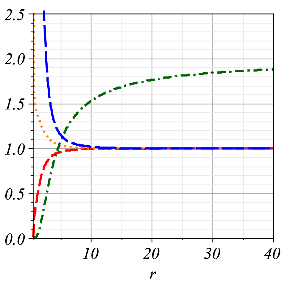


We see no qualitative difference in behavior in that appear to be monotonic regardless of whether or (we omit plots for , as these look very similar too).
Another way to analyze the solutions is to look at log-log plots of the metric functions and fields for a small value of . For this, we expect to see a section closely approximating the pure Lifshitz spacetime, and indeed this is what we find. We plot an example of this in figure 3.

Finally, we turn to the matter of the energy density. From the AdS asymptotics we read that the energy density is
| (88) |
where we have already set ). Therefore
| (89) |
is a unitless measure of the energy, and where we have denoted when . We plot this in figure 4.

Next, we will argue on general grounds that this expression for the energy density should be expected. First, we recall a few facts,
| (90) |
Now, in the energy density we have a term and a term . Further, is the value of the potential at the boundary (after we fix at the boundary), and is a global symmetry invariant (under shifting of and ). In deriving the above, we have assumed that asymptotes to , fixing the time rescaling. Finally, the above observations allows us to write
| (91) |
In fact, we can derive such a relationship using only conformal symmetry. We note that and are energies, and are densities, and is an energy density. Hence, we expect that in spatial dimensions these quantities should scale as
| (92) |
and so the general functional form must be
| (93) |
Next, we assume the first law of thermodynamics
| (94) |
We take the above differentials and equate the coefficient to find
| (95) |
and equate the coefficient to find
| (96) |
Using (95) this reads
| (97) |
which is identical to
| (98) |
Further, the relationship (95) becomes
| (99) |
or rearranging a bit
| (100) |
The generalization of the above argument for arbitrary number of particle species is straightforward, and gives
| (101) |
Using this, and the Euler relation we arrive at the familiar : the stress-energy tensor is traceless.
For the case at hand, the argument is reversible, i.e. the scaling relation can be obtained from a relation of the sort
| (102) |
Again, we assume the first law of thermodynamics
| (103) |
and write all functions in terms of the thermodynamic variables and find
| (104) | |||||
Equating differentials allows us to write two first order differential equations
| (105) | |||
| (106) |
Taking the integrability condition for these two equations ( acting on the first equation minus acting on the second) we find that
| (107) |
which is the same relation as the one above (100). This allows us to separate the equations and find
| (108) | |||
| (109) |
The above differential equations have the following solutions
| (110) |
(these functions are related easily to and above) and the integrability condition (107) relates to via
| (111) |
Next, we would like to know what initial set of data specifies the thermodynamics in the entire plane. More specifically, we already know that we have a solution for the case (this is the uncharged black brane in AdS case), and would like to know if this, or any additional information, can specify the thermodynamics off of this curve. To do so, we would like to calculate the characteristic equation for paths in space, parametrically given by . The characteristic curves are those that satisfy
| (112) |
(we note that the characteristic equations are the same for both of our linear PDEs). The most general solution to these equations, up to reparameterization of , are
| (113) |
These curves are given by . These are either hyperbola-like curves that do not intersect or (the degenerate case being the “hyperbola-like” curve ), or they are power law curves that go through the origin at (degenerate cases given by or ), depending on the particular values of and . For us we have so that lines of constant are related, which matches the scaling argument above.
Note that the curve is a characteristic curve, simply setting . This means that the initial conditions provided by the curve are not sufficient to determine the functions and off of the curve (see for example [41]). Further, no amount of additional perturbative information will yield a complete amount of information off a characteristic curve. This is realized by the presence of the general function in the general solutions (110). This basically comes down to saying something that we already knew: all relevant information differentiating models depends on (again, for AdS). This is reflected in the geometry by saying that defines a scale, and defines a scale and all solutions related by rescaling are related by the diffeomorphism that leave the AdS asymptotics alone, but shift the relevant scales in the bulk. What we have learned is that no amount of perturbative information around a solution can fix the thermodynamics. This is good because there are many different holographic models with a gauge invariance, all of which presumably have different thermal behavior.
Finally note that along a characteristic curve, the functions and are constant. This allows us to quickly deduce that along a characteristic curve, , . For us . Calling we find that the scaling becomes . This is just the scaling in AdSd+2 noted above (the scaling of follows from (98)).
To summarize, we believe that the above arguments are general enough to apply to a theory where the only two scales are the chemical potential and the temperature , and where the theory has a conformally invariant UV fixed point. Under these conditions, we expect (98) to hold, and that the different models are parameterized by the functions (say) . This information is beyond relation (98), i.e. it is information off of the characteristic curves that it defines.
We end by mentioning some possible future directions:
- 1.
It would be interesting to explore the space of models with different functions .
- 2.
One could study field theories on a dimensional sphere, i.e. the black hole geometries with spherical horizon. In these cases we expect phase transitions.
- 3.
Other dimensions: one could expect there to be different thermal behavior, possibly phase transitions, for general , as discussed at the end of section 1.
- 4.
One could calculate certain correlation functions in the dual theory, and see how they interpolate between non-relativistic and relativistic behavior.
- 5.
One could also study the dyonically charged versions of these black holes. There should be constant dilaton solutions where the magnetic and electric charge are equal (see [42] for a recent study).
- 6.
One could also study theories that asymptote to the Lifshitz-like background and are charged under a different field (essentially adding a scale in the Lifshitz background). However, note the curious result in [43] where an analytic charged solution is found, but the potential diverges. It would be interesting to see if there are solutions with a finite (chemical) potential. Using similar scaling arguments, we expect that a relationship of the type (102) can be written in such a case with . However, we would like to back this up with an explicit calculation.
Acknowledgements
We wish to thank Bob Holdom for programming tips in maple, and Ida G. Zadeh who was involved in early stages of this project. This work was supported by NSERC Canada.
References
- [1] J. M. Maldacena, Adv. Theor. Math. Phys. 2, 231 (1998) [Int. J. Theor. Phys. 38, 1113 (1999)], [arXiv:hep-th/9711200] E. Witten, Adv. Theor. Math. Phys. 2, 253 (1998) [arXiv:hep-th/9802150].
- [2] O. Aharony, S. S. Gubser, J. M. Maldacena, H. Ooguri and Y. Oz, Phys. Rept. 323, 183 (2000) [arXiv:hep-th/9905111].
- [3] Y. Oz and J. Terning, Nucl. Phys. B 532, 163 (1998) [arXiv:hep-th/9803167]. S. Kachru and E. Silverstein, Phys. Rev. Lett. 80, 4855 (1998) [arXiv:hep-th/9802183]. A. E. Lawrence, N. Nekrasov and C. Vafa, Nucl. Phys. B 533, 199 (1998) [arXiv:hep-th/9803015]. I. R. Klebanov and E. Witten, Nucl. Phys. B 536, 199 (1998) [arXiv:hep-th/9807080]. S. Benvenuti, S. Franco, A. Hanany, D. Martelli and J. Sparks, JHEP 0506, 064 (2005) [arXiv:hep-th/0411264]. A. Butti, D. Forcella and A. Zaffaroni, JHEP 0509, 018 (2005) [arXiv:hep-th/0505220]. S. Franco, A. Hanany, D. Martelli, J. Sparks, D. Vegh and B. Wecht, JHEP 0601, 128 (2006) [arXiv:hep-th/0505211].
- [4] I. R. Klebanov and M. J. Strassler, JHEP 0008, 052 (2000) [arXiv:hep-th/0007191]. J. M. Maldacena and C. Nunez, Phys. Rev. Lett. 86, 588 (2001) [arXiv:hep-th/0008001]. T. Sakai and S. Sugimoto, Prog. Theor. Phys. 113, 843 (2005) [arXiv:hep-th/0412141]. T. Sakai and S. Sugimoto, Prog. Theor. Phys. 114, 1083 (2005) [arXiv:hep-th/0507073].
- [5] J. Polchinski and M. J. Strassler, Phys. Rev. Lett. 88, 031601 (2002) [arXiv:hep-th/0109174]. H. Boschi-Filho and N. R. F. Braga, JHEP 0305, 009 (2003) [arXiv:hep-th/0212207]. J. Erlich, E. Katz, D. T. Son and M. A. Stephanov, Phys. Rev. Lett. 95, 261602 (2005) [arXiv:hep-ph/0501128]. L. Da Rold and A. Pomarol, Nucl. Phys. B 721, 79 (2005) [arXiv:hep-ph/0501218].
- [6] S. W. Hawking and D. N. Page, Commun. Math. Phys. 87, 577 (1983). A. Chamblin, R. Emparan, C. V. Johnson and R. C. Myers, Phys. Rev. D 60, 064018 (1999) [arXiv:hep-th/9902170]. M. Cvetic and S. S. Gubser, JHEP 9904, 024 (1999) [arXiv:hep-th/9902195].
- [7] D. T. Son, Phys. Rev. D 78, 046003 (2008) [arXiv:0804.3972 [hep-th]].
- [8] K. Balasubramanian and J. McGreevy, Phys. Rev. Lett. 101, 061601 (2008) [arXiv:0804.4053 [hep-th]].
- [9] T. Albash and C. V. Johnson, arXiv:0907.5406 [hep-th]. P. Basu, J. He, A. Mukherjee and H. H. Shieh, arXiv:0908.1436 [hep-th]. S. S. Gubser, F. D. Rocha and P. Talavera, arXiv:0911.3632 [hep-th]. S. A. Hartnoll and D. M. Hofman, arXiv:0912.0008 [cond-mat.str-el]. T. Faulkner, N. Iqbal, H. Liu, J. McGreevy and D. Vegh, arXiv:1003.1728 [hep-th]. B. H. Lee, D. W. Pang and C. Park, arXiv:1006.1719 [hep-th]. L. Y. Hung, D. P. Jatkar and A. Sinha, arXiv:1006.3762 [hep-th]. C. Hoyos-Badajoz, A. O’Bannon and J. M. S. Wu, arXiv:1007.0590 [hep-th].
- [10] S. A. Hartnoll, arXiv:0903.3246 [hep-th]. C. P. Herzog, arXiv:0904.1975 [hep-th].
- [11] P. Koroteev and M. Libanov, JHEP 0802, 104 (2008) [arXiv:0712.1136 [hep-th]]. P. Koroteev and M. Libanov, Phys. Rev. D 79, 045023 (2009) [arXiv:0901.4347 [hep-th]].
- [12] S. Schafer-Nameki, M. Yamazaki and K. Yoshida, JHEP 0905 (2009) 038 [arXiv:0903.4245 [hep-th]].
- [13] A. Adams, K. Balasubramanian and J. McGreevy, JHEP 0811, 059 (2008) [arXiv:0807.1111 [hep-th]]. C. P. Herzog, M. Rangamani and S. F. Ross, JHEP 0811, 080 (2008) [arXiv:0807.1099 [hep-th]]. J. Maldacena, D. Martelli and Y. Tachikawa, JHEP 0810, 072 (2008) [arXiv:0807.1100 [hep-th]]. D. Yamada, Class. Quant. Grav. 26, 075006 (2009) [arXiv:0809.4928 [hep-th]]. L. Mazzucato, Y. Oz and S. Theisen, JHEP 0904, 073 (2009) [arXiv:0810.3673 [hep-th]]. A. Donos and J. P. Gauntlett, JHEP 0903, 138 (2009) [arXiv:0901.0818 [hep-th]].
- [14] N. Bobev, A. Kundu and K. Pilch, JHEP 0907, 107 (2009) [arXiv:0905.0673 [hep-th]]. A. Donos and J. P. Gauntlett, N. Bobev, A. Kundu and K. Pilch, arXiv:0905.0673 [hep-th]. JHEP 0907, 042 (2009) [arXiv:0905.1098 [hep-th]]. E. Imeroni and A. Sinha, JHEP 0909, 096 (2009) [arXiv:0907.1892 [hep-th]].
- [15] T. Azeyanagi, W. Li and T. Takayanagi, JHEP 0906, 084 (2009) [arXiv:0905.0688 [hep-th]].
- [16] S. A. Hartnoll, J. Polchinski, E. Silverstein and D. Tong, JHEP 1004, 120 (2010) [arXiv:0912.1061 [hep-th]].
- [17] J. Blaback, U. H. Danielsson and T. Van Riet, JHEP 1002, 095 (2010) [arXiv:1001.4945 [hep-th]].
- [18] S. Kachru, X. Liu and M. Mulligan, Phys. Rev. D 78, 106005 (2008) [arXiv:0808.1725 [hep-th]].
- [19] M. Taylor, arXiv:0812.0530 [hep-th].
- [20] R. G. Cai, Y. Liu and Y. W. Sun, JHEP 0910, 080 (2009) [arXiv:0909.2807 [hep-th]]. Y. S. Myung, Y. W. Kim and Y. J. Park, arXiv:0910.4428 [hep-th]. M. C. N. Cheng, S. A. Hartnoll and C. A. Keeler, JHEP 1003, 062 (2010) [arXiv:0912.2784 [hep-th]]. E. Ayon-Beato, A. Garbarz, G. Giribet and M. Hassaine, JHEP 1004, 030 (2010) [arXiv:1001.2361 [hep-th]].
- [21] C. M. Chen and D. W. Pang, JHEP 1006, 093 (2010) [arXiv:1003.5064 [hep-th]].
- [22] U. H. Danielsson and L. Thorlacius, arXiv:0812.5088 [hep-th].
- [23] R. B. Mann, arXiv:0905.1136 [hep-th].
- [24] G. Bertoldi, B. A. Burrington and A. Peet, Phys. Rev. D 80, 126003 (2009) [arXiv:0905.3183 [hep-th]].
- [25] G. Bertoldi, B. A. Burrington and A. W. Peet, Phys. Rev. D 80, 126004 (2009) [arXiv:0907.4755 [hep-th]].
- [26] M. H. Dehghani and R. B. Mann, arXiv:1006.3510 [hep-th].
- [27] K. Balasubramanian and J. McGreevy, Phys. Rev. D 80, 104039 (2009) [arXiv:0909.0263 [hep-th]].
- [28] E. J. Brynjolfsson, U. H. Danielsson, L. Thorlacius and T. Zingg, J. Phys. A 43, 065401 (2010) [arXiv:0908.2611 [hep-th]]. M. H. Dehghani and R. B. Mann, arXiv:1004.4397 [hep-th].
- [29] S. F. Ross and O. Saremi, arXiv:0907.1846 [hep-th].
- [30] D. W. Pang, arXiv:0905.2678 [hep-th].
- [31] K. Goldstein, S. Kachru, S. Prakash and S. P. Trivedi, arXiv:0911.3586 [hep-th].
- [32] F. Aprile, S. Franco, D. Rodriguez-Gomez and J. G. Russo, JHEP 1005, 102 (2010) [arXiv:1003.4487 [hep-th]].
- [33] C. Charmousis, B. Gouteraux, B. S. Kim, E. Kiritsis and R. Meyer, arXiv:1005.4690 [hep-th].
- [34] Y. Liu and Y. W. Sun, arXiv:1006.2726 [hep-th].
- [35] K. B. Fadafan, arXiv:0912.4873 [hep-th].
- [36] S. J. Sin, S. S. Xu and Y. Zhou, arXiv:0909.4857 [hep-th].
- [37] M. Cadoni, G. D’Appollonio and P. Pani, JHEP 1003, 100 (2010) [arXiv:0912.3520 [hep-th]].
- [38] D. Anninos, S. A. Hartnoll and N. Iqbal, arXiv:1005.1973 [hep-th].
- [39] A. Batrachenko, J. T. Liu, R. McNees, W. A. Sabra and W. Y. Wen, JHEP 0505, 034 (2005) [arXiv:hep-th/0408205].
- [40] S. S. Gubser and F. D. Rocha, Phys. Rev. D 81, 046001 (2010) [arXiv:0911.2898 [hep-th]].
- [41]
E. C. Zachmanoglou,
Mineola, N.Y. USA: Dover Publications, Inc. (1998) 393 p. - [42] E. Gubankova, arXiv:1006.4789 [hep-th].
- [43] D. W. Pang, JHEP 1001, 116 (2010) [arXiv:0911.2777 [hep-th]].