Detecting Local Network Motifs

We consider a network $G$ of interest on $n$ vertices. In this work, we consider directed graphs, with possible loops and opposite edges, but all the results can easily be extended to undirected graphs.

A pattern $\mathbf{m}$ of size $k$ is a directed graph on $k$ vertices, from which we want to know if it is locally over-represented in $G$. As a convention, we will denote by $(a,b,\dots)$ the vertices of $\mathbf{m}$ and by $(u,v,\ldots)$ those of $G$.

An automorphism of $\mathbf{m}$ is a permutation $\phi$ of its vertices such that, for every pair $(a,b)$ of vertices, $\overrightarrow{\phi(a)\phi(b)}$ is an edge if and only if $\overrightarrow{ab}$ is an edge. Let $\mathcal{R}$ be the relation defined by $a\mathcal{R}b$ if $b$ is the image of $a$ by an automorphism. $\mathcal{R}$ is an equivalence relation on the vertices of $\mathbf{m}$ and those vertices can therefore be partitioned into equivalence classes, which we call deletion classes. For example, in the bi-fan pattern shown in Figure 1, the permutation exchanging $a$ with $b$ and $c$ with $d$ is an isomorphism. However, $a$ and $c$ are not equivalent as they have different outdegrees. Thus the bi-fan has two deletion classes which are $\{a,b\}$ and $\{c,d\}$.

Let $(C_{1},\ldots,C_{K})$ be the deletion classes of $\mathbf{m}$ and $(i_{1},\ldots,i_{K})$ their respective sizes. A position $U$ in a network $G$ for $\mathbf{m}$ will then denote a list $(V_{1},\ldots,V_{K})$ of disjoint sets of vertices of $G$ with respective sizes $(i_{1},\ldots,i_{K})$. That position is an occurrence of $\mathbf{m}$ in $G$ if the subgraph of $G$ induced by the vertices of $U$ is isomorphic to $\mathbf{m}$. Writing a position as a list of sets of vertices ensures to count every occurrence of a pattern only once. However, for clarity, we will write positions as lists of vertices throughout the article.

A subpattern of $\mathbf{m}$ denotes a pair $(C,\mathbf{m}^{\prime})$, where $C$ is a deletion class of $\mathbf{m}$ and $\mathbf{m}^{\prime}$ the pattern on $k-1$ vertices obtained by deleting any vertex of $C$. As all vertices in $C$ are isomorphic, their respective deletion lead to isomorphic subgraphs and the notion of subpattern is thus well defined.

However, the opposite is not true, that is the subgraphs of $\mathbf{m}$ obtained by deleting a vertex $a$ or a vertex $b$ may be isomorphic while $a$ and $b$ do not belong to the same deletion class. Consider for example the feed-forward loop shown in Figure 1. Deleting any of its three vertices leads to a single edge but all the vertices belong to different deletion classes as they are not topologically equivalent (they have for instance different out-degrees).

In the following, we adopt the graphical convention shown in the last column of Figure 1 to draw at the same time a pattern $\mathbf{m}$ and one of its subpatterns $(C,\mathbf{m}^{\prime})$. The whole graph represents $\mathbf{m}$ and the squared vertex whose adjacent edges are dotted is a vertex of $C$. The pattern $\mathbf{m}^{\prime}$ is thus obtained by deleting that vertex.

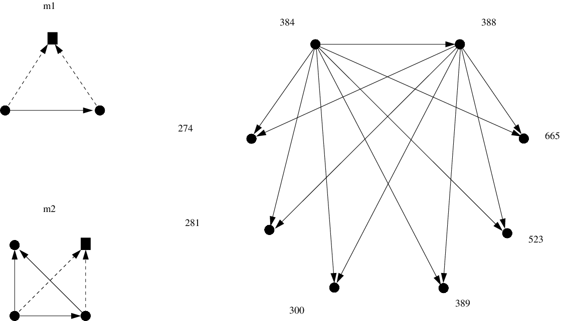
Let $\mathbf{m}$ be a pattern and $(C,\mathbf{m}^{\prime})$ one of its subpatterns. An occurrence $U$ of $\mathbf{m}$ in $G$ is an extension of an occurrence $U^{\prime}$ of $\mathbf{m}^{\prime}$ if the vertex set of $U^{\prime}$ is a subset of the vertex set of $U$ . We define the $(\mathbf{m},C$)-theme on $U^{\prime}$ as the subgraph of the network induced by the occurrence of $\mathbf{m}^{\prime}$ at $U^{\prime}$ and all its extensions. The number of those extensions will be the order of the theme (see Figure 2 for an illustration).

We define a potential local motif as a pattern which is locally over-represented with respect to at least one of its subpatterns. In other words, $\mathbf{m}$ is a potential local motif with respect to $(C,\mathbf{m}^{\prime})$ if there exist an $(\mathbf{m},C)$-theme whose order is significantly higher than the expected order in a random model to be specified in Section 2.2. Note that the local over-representation is different from the global one. Indeed, a pattern having a high number of disjoint occurrences may be globally over-represented without being a motif according to our definition. On the other hand, a pattern may be locally over-represented without having a large number of occurrences in the whole network.

Finally, a potential local motif is a local motif if the information it conveys is not redundant with a smaller local motif, that is if it is not filtered out by the procedure to be described in subsection 2.5.

The random generation model we consider is based on blockmodels (White, Boorman and Breiger, 1976), with a fixed and known class for each vertex and random edges. It depends on a $4$-tuple of parameters $(n,Q,\mathbf{Z},\mathbf{\Pi)}$, where:

• •

  $n$ is the number of vertices,

• •

  $Q$ is the number of classes of the model,

• •

  $\mathbf{Z}\in\{1,\ldots,Q\}^{n}$ is a vector giving the class of each vertex,

• •

  $\mathbf{\Pi}$ is a $Q\times Q$ connectivity matrix. The coefficient $\Pi_{ql}\in[0,1]$ of that matrix indicates how likely a vertex of class $q$ and a vertex of class $l$ are linked by an edge.

Under this model, all the edges of the random graph are drawn independently under Bernoulli laws: denoting by $X_{uv}$ the indicator variable of the edge between vertices $u$ and $v$,

Such a model belongs to the family of blockmodels, which are widely used to describe real network data (Nowicki and Snijders, 2001). It has at least two main advantages. First, it takes into account the preferential attachment process between several groups of nodes in the network; second, as all the edges are independent, calculations remain tractable.

Note that it is not the classical random graph model introduced by Erdős and Rényi (1959) as the edge probabilities are non uniform (unless $Q=1$). It is neither a mixture model as the classes of the vertices are not random. Adding randomness on the classes would induce correlations between the edges and therefore invalidate the Poisson approximation of Section 2.3.

Nevertheless, the vertex classes and the connectivity matrix $\Pi$ may be inferred using estimation algorithms for graph mixtures (Nowicki and Snijders, 2001; Daudin, Picard and Robin, 2008; Hofman and Wiggins, 2008; Latouche, Birmelé and Ambroise, 2008). The graph mixture models, when applied for $Q$ components in the mixture, infer for each vertex a vector of length $Q$ giving the probability for that vertex to belong to each class, as well as a connectivity matrix. We choose here to assign each vertex to its more probable class, and thus deal with the the observed network as if the groups were known and fixed.

Our general random graph framework also contains another widely used model where $u$ and $v$ are linked with probability proportional to the product of their respective observed degrees. Under that model, which we will call Expected Degree, the expected degree of each vertex is almost equal to its observed degree (Matias et al., 2006). However, under this model, nodes are in the same class if and only if they have the same in- and outdegrees. Therefore, the number of classes may be large on real networks, having a deep impact on the running time of our motif detection procedure.

Overlapping classes can also be taken into account by using for instance the Mixed Membership Stochastic Blockmodel from Airoldi et al. (2008) or the model Overlapping Stochastic Blockmodel from Latouche, Birmelé and Ambroise (to appear).

Consider a pattern $\mathbf{m}$ of size $k$, a subpattern $(C,\mathbf{m}^{\prime})$ of $\mathbf{m}$ and a set $U$ of $k-1$ vertices in some graph $G$. If $U$ corresponds to an occurrence of $\mathbf{m}^{\prime}$, we write $G[U]\sim\mathbf{m}^{\prime}$. Let $N_{U}(\mathbf{m})$ denote the order of the $(\mathbf{m},C)$-theme located at $U$. If $U$ does not correspond to an occurrence of $\mathbf{m}^{\prime}$, we set $N_{U}(\mathbf{m})=0$.

We define $\lambda_{U}(\mathbf{m})=\mathbb{E}(N_{U}(\mathbf{m})|G[U]\sim\mathbf{m}^{\prime})$ and $\Delta_{U}(\mathbf{m})$ as the normalized quantity

Looking for themes whose order is much larger than expected under our model is then equivalent to look for values of $\Delta_{U}(\mathbf{m})$ significantly larger than $1$.

In the following, we will omit the reference to $\mathbf{m}$ when there is no ambiguity.

Let us consider a set $U$ corresponding to an occurrence of $\mathbf{m}^{\prime}$. For each vertex $v\notin U$, we denote by $I_{U}^{v}$ the indicator random variable which is equal to $1$ if adding $v$ to $U$ yields an occurrence of $\mathbf{m}$ in $G$. Let $p_{U}^{v}$ be the mean value of $I_{U}^{v}$. Then $\lambda_{U}=\sum_{v\notin U}p_{U}^{v}$ and those quantities can easily be deduced from the parameters of the random graph model.

As the indicator random variables $(I_{U}^{v})_{v\notin U}$ are independent, it is well known that the law of their sum, that is the law of $N_{U}$, can be approximated by a Poisson law (Barbour, Holst and Janson, 1992). More precisely, denoting by $d_{TV}$ the total variation distance between two distributions, we have

where $\mathcal{L}(Po(\lambda_{U}))$ is the Poisson distribution with parameter $\lambda_{U}$.

This approximation may be used to determine an upper bound for the $p$-value of testing if the $(\mathbf{m},C)$-theme order is surprisingly large. In practice, such bounds are quite accurate as the $p_{U}^{v}$’s are small.

Nevertheless, a better approximation can be obtained for the tail probabilities by using Chen-Stein’s method (Chen, 1975), as shown in Barbour, Holst and Janson.

where, for any measurable set $A$, $Po(\lambda_{U})(A)$ is the probability of $A$ under the Poisson distribution with parameter $\lambda_{U}$.

Setting $K=\lceil\lambda_{U}(1+t)\rceil$ for some $t>1$ and using elementary bounds and transformations developed in Appendix A, we obtain

For positive values of $t$ which are smaller than or close to $1$, a sharper bound can be obtained by using a concentration inequality on the sum of independent random variables bounded between $0$ and $1$ (McDiarmid, 1998).

Moreover, it is straightforward to verify that the function of $t$ defined on $]1,+\infty[$ by $\frac{\sqrt{t+1}}{\sqrt{2\pi\lambda}(t-1)}$ is decreasing and is equal to $1$ at

Therefore, coupling inequalities (2.2) and (2.3) yields a local bound for the tail probability of the theme order.

We thus have an exponentially decreasing local bound for the tail probability of the centered and renormalized order of an $(\mathbf{m},C)$-theme on $U$. Moreover, that bound is easily computable from the parameters of the random graph model.

Theorem 2.1 allows to test whether there is a local over-representation at a given position $U$ of an $(m,C)$-theme. However, the number of possible positions $U$ is growing as $n^{k-1}$. We thus encounter a multiple testing problem. To overcome this issue, we build a statistic characterizing any local over-representation of a pattern somewhere in the graph.

Let us consider the function $g$ defined for every positive $\lambda$ and $t$ by

For any positive $\lambda$, the function $g(\lambda,.)$ is a one-to-one increasing function, mapping $]0,+\infty[$ to itself and which is equivalent to $\lambda t\log(t)$ as $t$ tends to infinity. Thus, the event $g(\lambda_{U},\Delta_{U})$ much larger than $1$ is equivalent to the event $\Delta_{U}$ much larger than $1$.

For any positive $t$, let us apply Theorem 2.1 to $y$ such that $g(\lambda_{U},y)=t$. We then obtain

Noting that the event $E^{t}=\{\max_{U}(g(\lambda_{U},\Delta_{U}))\geq t\}$ is the union over all the possible positions $U$ of the events $E^{t}_{U}=\{g(\lambda_{U},\Delta_{U})\geq t\}$, and that the exponential term in the upper bound is independent of $U$, we obtain our main result, stated in the following theorem.

We thus obtain an upper bound on the global $p$-value for detecting a local over-representation of $\mathbf{m}$ with respect to the subpattern $(C,\mathbf{m}^{\prime})$ occurring anywhere in the network.

Consider the two patterns and respective subpatterns of Figure 2. Let $C_{1}$ and $C_{2}$ denote the respective deletion classes of the subpatterns. Then, as shown by the figure, every $(\mathbf{m}_{2},C_{2})$-theme of order $K$ is an $(\mathbf{m}_{1},C_{1})$-theme of order $K+1$. In that case, the fact that the $(\mathbf{m}_{2},C_{2})$-theme is of order significantly larger than expected is redundant with the same information for the $(\mathbf{m}_{1},C_{1})$-theme.

To avoid such redundance in the final motif list, a pattern $\mathbf{m}$ will be considered as a motif with respect to a subpattern $(C,\mathbf{m}^{\prime})$ if the two following conditions hold:

1. 1.

   The $p$-value given by Theorem 2.2 is lower than a fixed threshold, that is $\mathbf{m}$ is a potential local motif;

2. 2.

   Let $\{a\}$ be a vertex of $C$. There exist no set $\mathcal{A}$ of vertices of $\mathbf{m}$ such that

   • •

     there is no edge between $a$ and any vertex of $\mathcal{A}$,

   • •

     $\mathbf{m}\setminus\mathcal{A}$ is over-represented with respect to $(D,\mathbf{m}\setminus(\mathcal{A}\cup\{a\})$, where $D$ is the deletion class of $\{a\}$ in $\mathbf{m}\setminus\mathcal{A}$ .

If there exists a set $\mathcal{A}$ satisfying the two points of the second condition, then the over-representation of $\mathbf{m}$ with respect to $(C,\mathbf{m}\setminus\{a\})$ is considered as redundant with the over-representation of $\mathbf{m}\setminus\mathcal{A}$ with respect to $(D,\mathbf{m}\setminus(\mathcal{A}\cup\{a\}))$. Thus, the pair $(\mathbf{m},C)$ is filtered out from the local motif list.

Figure 3 illustrates the filtering procedure. Moreover, it shows why the absence of any edge between vertex $a$ and set $\mathcal{A}$ is required to filter out a potential local motif. Indeed, consider the first pattern of the figure for which $\mathcal{A}=\{b\}$ fulfills the previous condition. The corresponding theme doesn’t convey any new information compared to the theme of the feed-forward loop obtained by deleting the vertex $w$.

On the opposite, a theme of order $k$ of the second pattern contains $k$ supplementary edges compared to the feed-forward loop theme. The coefficients of $\mathbf{\Pi}$ being small in general because of the sparsity of real networks, the presence of those $k$ edges is informative. Thus, that potential local motif is kept in the list of local motifs.

Given an integer value $k$, our procedure first needs to list all the patterns of size $k$ occirring in the network, as well as their subpatterns. That issue is tackled by using the ESU algorithm of Wernicke (2005). It is important to note that this subgraph count has only to be done on the observed graph and not on a huge number of simulated ones.

We then apply Theorem 2.2 to each pair (pattern, subpattern). The major cost in terms of computational time of that step is the computation of $\mathbb{E}(N(\mathbf{m}^{\prime}))$. Indeed, it requires to sum a probability of occurrence along all possible positions in the graph. It may be done more efficiently by grouping the nodes belonging to the same class. This approach gives good results when the number of classes is not too large, which is the case in practice when estimating the classes using mixture models algorithms. However, it becomes a real drawback for motifs larger than $4$ vertices when using the Expected Degree method and observed graph with more than $200$ vertices.

Finally, as the algorithm visits every position, it is not time-consuming to keep in memory all the positions and their respective theme orders in order to have a better interpretation of the results.

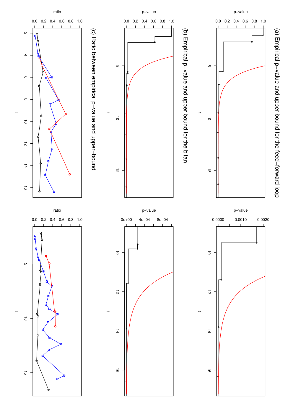
$500,000$ directed graphs with $90$ vertices, which we will call the reference graphs, were generated under the model with three classes of $30$ vertices each and connection probabilities set to $0.04$ between vertices of the same class and $0.01$ between vertices of different classes. The mean out-degree and in-degree under that model are both equal to $1.76$. Our method is illustrated with the feed-forward loop an the bi-fan patterns (see Figure 1). The choice of the subpatterns is done by deleting the only vertex of in-degree $2$ for the feed-forward loop and one of the vertices of in-degree $2$ for the bi-fan. Nevertheless, that choice plays no role in that particular case, due to the symmetry of the model. Figure 4 (a) and (b) show the empirical tail probabilities and corresponding upper bounds given by Theorem 2.2, as functions of the parameter $t$.

To evaluate the quality of the upper bound, the ratio between the empirical $p$-values and their upper bounds is shown in Figure 4 (c). The same ratio is also plotted for more dense graphs ($30,000$ graphs sampled with the same number of nodes and classes and connection probabilities five times larger) and for graphs larger than the reference graphs but with comparable density ($30,000$ graphs with $360$ nodes, three classes of $120$ nodes each and connection probabilities $0.01$ and $0.0025$). For the reference graphs, the ratio is about $1/10$ for both patterns, with a minimum of $0.07$ for the feed-forward loop and $0.04$ for the bi-fan. This ratio increases both for larger graphs and more dense graphs.

The $p$-value used to decide if a pattern is a motif or not depends on the inferred connection matrix $\mathbf{\Pi}$. To evaluate the incidence of the choice of the inference method, the motif search is run for four distinct models:

• •

  the Erdős-Rényi model (Erdős and Rényi, 1959) with a connection probability such that the expected number of edges is equal to the observed one;

• •

  the Expected Degree (ED) model described in Matias et al.. That model draws a link between vertices $u$ and $v$ with a probability proportional to $d_{u}d_{v}$, where $d_{u}$ denotes the observed degree of the node $u$. An adequate choice of the normalisation constant leads to a model for which the expected degree of each node is almost equal to its observed one;

• •

  the mixture model MixNet in its Bayesian version (Latouche, Birmelé and Ambroise, 2008) implemented in the mixer R-package;

• •

  the mixture model BLOCKS (Nowicki and Snijders, 2001) available in the STOCNET software (http://stat.gamma.rug.nl/stocnet/).

As BLOCKS only supports graphs up to $200$ nodes, we consider a randomly chosen subnetwork of the transcriptional Yeast regulation network containing $194$ nodes. Inference of the matrix $\mathbf{\Pi}$ and search for all local motifs of size $3$ and $4$ is done on that subnetwork. Table 1 shows all the motifs found using a threshold of $0.05$ on the $p$-value with at least one of the method. One can see that the list of motifs remains stable.

The only method leading to significantly different $p$-values is the one relying on the Erdős-Rényi model, which is known to poorly describe real networks.

On the other hand, the method relying on the Expected Degree model is the one selecting the smallest number of motifs.The main difference with the two last methods is that the top-motif for Mixnet and BLOCKS is not a motif for ED. However, large themes for the bi-fan, which is detected as a motif by ED, correspond also to large themes of the first motif of size $3$. Thus, the themes pointed out by the three methods are the same ones.

Finally, the two methods taking into account both the degree-distribution and the group structure of networks, that is MixNet and BLOCKS, select the same motifs and with comparable $p$-values.

In order to point out the difference between global motifs and local ones, we run our procedure to determine all local motifs of size $3$, $4$ and $5$ in two standard networks, both studied in Milo et al., and publicly available at http://weizmann.ac.il/mcb/UriAlon. Those networks are the transcriptional regulatory networks of Yeast and the electronic circuit s420 of the ISCAS89 benchmark.

Inference of the parameters of the model is done using the Bayesian MixNet approach in order to be able to tackle patterns of size $5$ in those graphs. However, that choice implies that hubs may be grouped in the same class, which is relevant from a mixture model point of view but may generate quite inhomogeneous groups in terms of degrees and thus local motifs with poor biological interpretation. For example, the parameter inference on the Yeast network gives rise to a group of two hubs of respective out-degrees $71$ and $44$. Hence, the expected outdegree in that group is $57.5$ and any star pattern will be selected as a local motif when centering the position on the largest hub.

To avoid that phenomenon, we first run the whole procedure with the Bayesian MixNet approach and run it again with the Expected Degree approach when the position of the theme leading to a local motif shows that it is selected because of the presence of a vertex of high degree.

The algorithm is run on the Yeast regulatory network with a threshold of $1e-3$. Table 2 shows the local motifs of size $3$ found in the network, the row $N_{U}^{*}$ denoting the order of the theme at the position $U$ where $\Delta_{U}$ is maximal.

There are clearly two top local motifs of size $3$.

The first top local motif corresponds to a pair of regulators co-regulating a gene. This motif is not selected by the methods of global motif detection of Milo et al., Berg and Lässig or Wernicke and Rasche. However, all those methods select the motif of size $4$ called bi-fan (see Figure 1). That global over-representation of the bi-fan is a consequence of the the local motif we detect. Indeed, the three largest themes of our local motif are of respective orders $38$, $32$ and $18$. Thus, their presence imply ${38\choose 2}+{32\choose 2}+{18\choose 2}=1352$ occurrences of the bi-fan. As the total number of occurrences of the bi-fan in the network is $1843$, it gives confirmation on the local character of the over-representation of that pattern.

The second one is the feed-forward loop with respect to the deletion of the vertex in-degree $2$. A feed-forward is composed by a main regulator $X$ and a gene $Y$ regulated by $X$, both co-regulating a third gene $Z$. This pattern is a local motif with respect to the subpattern obtained by deleting $Z$. This indicates the existence of places in the network where a main regulator $X$ and a gene $Y$ regulated by $X$ both co-regulate a high number of genes $Z_{1},\ldots,Z_{k}$. The value of $N_{U}^{*}$ indicates that there is at least such a theme of order $38$. That phenomenon is already described by U. Alon (Alon, 2007), under the denomination Multi-output feed-forward loops.

The feed-forward loop is also found to be a local motif with respect to the deletion of the main regulator $X$. However, the $p$-value upper bound indicates that the order of the corresponding themes is less significative than in the previous case. This fact is confirmed by the lower value of $N_{U}^{*}$. It illustrates a main point of our method which is to differentiate the behaviour of the different deletion classes of a pattern.

Finally, the feed-forward loop is not a local motif with respect to the deletion of the intermediate gene $Y$, indicating that no main regulator $X$ regulates a high number of genes $Y_{1}\ldots Y_{k}$ in order to regulate a gene $Z$.

The method finds five local motifs of size $4$ in the Yeast regulatory network. They are shown in Table 3.

The first motif appearing in the list is of interest as it corresponds to three regulators co-regulating seven genes with an additional regulation between two of them. Another way to see the theme of that motif is a multi-output feed forward loop of order $7$ with a third regulator acting on $Z_{1},\ldots,Z_{7}$. That motif is also found by the global methods but with a higher $p$-value and at the fifth or sixth position among the motifs of size $4$.

The $4$ other local motifs have a value of $N_{U}^{*}$ lower than $2$, suggesting that they appear in the list because of a very low expected value. Note that the bi-fan does not appear in the list as it is filtered out as a redundancy of the second motif of size $3$.

Finally, there is only one local motif of size $5$. It corresponds to the fourth motif of size $4$ with a supplementary edge going out from the squared vertex. Its value for $N_{U}^{*}$ is $1$, showing that its expected is low, such that it becomes over-represented even at its first occurence.

The second network, that is the electronic circuit, has no local motif of size $3$, $4$ or $5$ relying on a threshold of $.01$. However, one global motif of size $3$ and two global motifs of size $4$ were found in Milo et al. with $Z$-scores larger than $10$. This indicates a distinct behaviour of the two types of networks, the occurrences of the global motifs of the electronic network being spread in the whole networks rather then agglomerated.

The first step is to find the best possible bound for the difference between the tail probability of a sum of independent random variables and the tail probability of the corresponding Poisson approximation. This problem is presented and studied in Barbour, Holst and Janson (1992). We use Theorem 9.D presented in that book, namely

Applying this result in our context for $W=N_{U}$ and $K=\lceil\lambda_{U}(1+t)\rceil$ for a fixed $t$ may not be possible because in this case $\Gamma=t\sqrt{\lambda_{U}}$ and thus the condition $\Gamma\geq 1$ may not be satisfied when $\lambda_{U}$ is too small with respect to $t$.

However, the proof of Theorem B.1 uses the assumption $\Gamma\geq 1$ only once. Rewriting it without that condition until that step yields:

with

and

where $|\epsilon_{r}|\leq 8\xi\Gamma^{2}+2(r-K)\xi\Gamma\lambda^{-1/2}$.

The hypothesis $\Gamma\geq 1$ is then used to bound the right hand side of Inequality (B.2), which can be alternatively bounded by

the last inequality deriving from the fact that the ratio between two consecutive terms of the sum is always lower than $\lambda/K$.

Using the additional condition of Proposition 3.1, that is $K\geq 2\lambda_{U}$, and the fact that it implies $\Gamma\lambda^{-1/2}\geq 1$ allows us, using elementary bounds, to obtain from Inequalities (B.1) and (B.2) that

As $\xi\Gamma^{2}\leq\frac{K\lambda_{2}}{\lambda^{2}}$, we have

The second part of the right hand-side of Proposition 3.1 comes from the asymptotic comparison between the tail probability $Po(\lambda)\{[\lambda_{U}(1+t),+\infty)\}$ and its exponential approximation used in Theorem 2.1. It is derived in a very similar way than in Appendix A, using the following lower bound on $K!$, which can be proved from its asymptotic expansion

Proof: We start from the simplest known lower bound for the probability of an union of events, that is:

Given two positions $U$ and $V$, let $K_{U}$ and $K_{V}$ be such that $E^{t}_{U}=\{N_{U}(\mathbf{m})\geq K_{U}\}$ and $E^{t}_{V}=\{N_{V}(\mathbf{m})\geq K_{V}\}$. Moreover, let $ext(U)$ be the set of vertices yielding to extensions of $\mathbf{m}^{\prime}$ on $U$ and $i=|V\setminus U|$. Let us also recall that $k$ is the size of the pattern $\mathbf{m}$.

Let $S$ be any set of vertices not intersecting $U$. We decompose $E^{t}_{V}$ as the union of the sets $\{T\subset ext(V)\}$ for all sets $T$ of $K_{V}$ vertices. Thus

Let $T$ be such that $|T\cap S|=j$. As $\mathbf{m}^{\prime}$ is connected, at least $i$ edges need to be present in $V\setminus U$ to ensure that $G[V]\sim\mathbf{m}^{\prime}$. Moreover, to ensure that $T\subset ext(V)$, all the edges between $V\setminus U$ and $T$ and all the edges between $U\cap V$ and $T\setminus S$ have to be present, which amounts to a total of at least $iK_{V}+(k-i)(K_{V}-j)$ edges.

Therefore, denoting by $\rho$ the largest coefficient of the matrix $\mathbf{\Pi}$, $\mathbb{P}(T\subset ext(V)|ext(U)=S)\leq\rho^{i}\rho^{iK_{V}+(k-i)(K_{V}-j)}$.

We fix some $\epsilon>0$ and distinguish between two different cases whether the cardinality of $S$ is larger or smaller than $n^{\epsilon}$.

• •

  If $|S|\leq n^{\epsilon}$, then

  	$\displaystyle\mathbb{P}(E^{t}_{V}|ext(U)=S)$	$\displaystyle\leq$	$\displaystyle\sum_{j=0}^{min(|S|,K_{V})}{n\choose K_{V}-j}{|S|\choose j}\rho^{i+iK_{V}+(k-i)(K_{V}-j)}$		(B.5)
  		$\displaystyle\leq$	$\displaystyle\rho^{i+kK_{V}}n^{K_{V}}\sum_{j=0}^{K_{V}}{|S|\choose j}\big(\frac{1}{n\rho^{k-i}}\big)^{j}$
  		$\displaystyle\leq$	$\displaystyle\rho^{i+kK_{V}}n^{K_{V}}(K_{V}+1)\max(1,\big(\frac{1}{n\rho^{k-i}}\big)^{K_{V}})$
  		$\displaystyle\leq$	$\displaystyle\rho^{i}(K_{V}+1)\max\big(n\rho^{k},\rho^{i}|S|\big)^{K_{V}}$

  It is straightforward to check that, for large enough $n$, we have $n\rho^{k}<\frac{1}{e}$ and $\rho^{i}|S|<\frac{1}{e}$. Therefore, the right hand side of Inequality (B.5) is a decreasing function of $K_{V}$ and

  $$\mathbb{P}(E^{t}_{V}|ext(U)=S)\leq 2\max\big(n\rho^{i+k},\rho^{2i}|S|\big)$$

  Moreover, $1-(i+k)(\frac{1}{2}+\epsilon)\leq-i-(2k\epsilon-1)$ for $\epsilon\leq\frac{1}{2}$ and $-2i(\frac{1}{2}+\epsilon)+\epsilon=-i-\epsilon$. Thus, as $\rho\leq Cn^{-\frac{1}{2}-\epsilon}$ for some constant $C\geq 1$, and $|S|\leq n^{\epsilon}$,

  $$\mathbb{P}(E^{t}_{V}|ext(U)=S)\leq C^{2k}n^{-i-\delta}$$

  (B.6)

• •

  For $|S|\geq n^{\epsilon}$, we roughly bound $\mathbb{P}(E^{t}_{V}|ext(U)=S)$ by $1$. However, let us note that $g(\lambda_{U},n^{\epsilon})>n^{\epsilon}$ for large enough $n$ and therefore

  	$\displaystyle\sum_{S,|S|\geq n^{\epsilon}}\mathbb{P}(ext(U)=S)$	$\displaystyle=$	$\displaystyle\mathbb{P}(N_{U}\geq n^{\epsilon})$		(B.7)
  		$\displaystyle=$	$\displaystyle\mathbb{P}(g(\lambda_{U},N_{U})\geq g(\lambda_{U},n^{\epsilon}))$
  		$\displaystyle\leq$	$\displaystyle\mathbb{P}(g(\lambda_{U},N_{U})\geq n^{\epsilon})$
  		$\displaystyle\leq$	$\displaystyle\mathbb{P}(E^{t}_{U})e^{-n^{\epsilon}+t}\quad\mbox{ by Theorem~\ref{main}}$		(B.8)
  		$\displaystyle\leq$	$\displaystyle\mathbb{P}(E^{t}_{U})n^{-i-\delta}\quad\mbox{ for large enough }n.$		(B.9)

References

- Airoldi et al. (2008) [author] Airoldi, E.E., Blei, D.D., Fienberg, S.S. and Xing, E.E. (2008). Mixed membership stochastic blockmodels. Journal of Machine Learning Research 9 1981-2014.
- Alon (2007) [author] Alon, U.U. (2007). Network motifs: theory and experimental approaches. Nature Reviews Genetics 8 450-461.
- Artzy-Randrup et al. (2004) [author] Artzy-Randrup, Y.Y., Fleishman, S. J.S. J., Ben-Tal, N.N. and Stone, L.L. (2004). Comment on ”Network Motifs: Simple Building Blocks of Complex Networks” and ”Superfamilies of Evolved and Designed Networks”. Science 305.
- Banks et al. (2008) [author] Banks, EricE., Nabieva, ElenaE., Chazelle, BernardB. and Singh, MonaM. (2008). Organization of Physical Interactomes as Uncovered by Network Schemas. PLoS Comput. Biol. 4 e1000203.
- Barbour, Holst and Janson (1992) [author] Barbour, A. D.A. D., Holst, L.L. and Janson, S.S. (1992). Poisson approximation. Oxford University Press.
- Berg and Lässig (2004) [author] Berg, J.J. and Lässig, M.M. (2004). Local graph alignment and motif search in biological networks. Proc. Nat. Acad. Sci. 101 14689-14694.
- Chen (1975) [author] Chen, L. H. YL. H. Y. (1975). Poisson approximation for dependant trials. Ann. Probab. 3 534-545.
- Chung and Lu (2006) [author] Chung, F.F. and Lu, L.L. (2006). Complex Graphs and Networks (CBMS Regional Conference Series in Mathematics). AMS.
- Daudin, Picard and Robin (2008) [author] Daudin, J. J.J. J., Picard, F.F. and Robin, S.S. (2008). Mixture model for random graphs. Stat. Comput. 18 173-183.
- Dobrin et al. (2004) [author] Dobrin, R.R., Beg, Q. K.Q. K., Barabási, A. L.A. L. and Oltvai, Z. N.Z. N. (2004). Aggregation of topological motifs in Escherischia Coli transcriptional regulatory network. BMC Bioinformatics 5 10.
- Erdős and Rényi (1959) [author] Erdős, P.P. and Rényi, A.A. (1959). On random graphs I. Publ. Math. Debrecen 6 290-297.
- Hofman and Wiggins (2008) [author] Hofman, J.J. and Wiggins, C.C. (2008). Bayesian approach to network modularity. Phys. Rev. Lett. 100.
- Kashani et al. (2009) [author] Kashani, Z. R. M.Z. R. M., Ahrabian, H.H., Elahi, E.E., Nowzari-Dalini, A.A., Ansari, E. S.E. S., Asadi, S.S., Mohammadi, S.S., Schreiber, F.F. and Masoudi-Nejad, A.A. (2009). Kavosh: a new algorithm for finding network motifs. BMC Bioinformatics 10.
- Kashtan et al. (2004) [author] Kashtan, N.N., Itzkovitz, S.S., Milo, R.R. and Alon, U.U. (2004). Efficient sampling algorithm for estimating subgraph concentrations and detecting network motifs. Bioinformatics 20-11 1746.
- Latouche, Birmelé and Ambroise (2008) [author] Latouche, P.P., Birmelé, E.E. and Ambroise, C.C. (2008). Bayesian methods for graph clustering. SSB preprint 17.
- Latouche, Birmelé and Ambroise (to appear) [author] Latouche, P.P., Birmelé, E.E. and Ambroise, C.C. (to appear). Overlapping Stochastic Block Models. Ann. Appl. Stat.
- Matias et al. (2006) [author] Matias, C.C., Schbath, S.S., Birmelé, E.E., Daudin, J. J.J. J. and Robin, S.S. (2006). Network motifs: mean and variance for the count. REVSTAT 4 31-51.
- McDiarmid (1998) McDiarmid, C. (1998). Concentration. In Probabilistic Methods for Algorithmic Discrete Mathematics (J. R.-A. M. HabibC. McDiarmid and B. Reed, eds.) 195-248. Springer.
- Milo et al. (2002) [author] Milo, R.R., Shen-Orr, S.S., Itzkovitz, S.S., Kashtan, N.N., Chklovskii, D.D. and Alon, U.U. (2002). Network Motifs: Simple Building Blocks of Complex Networks. Science 298 824-827.
- Nowicki and Snijders (2001) [author] Nowicki, K.K. and Snijders, T. A. B.T. A. B. (2001). Estimation and prediction for stochastic block-structures. JASA 96 1077–87.
- Picard et al. (2008) [author] Picard, F.F., Daudin, J. J.J. J., Koskas, M.M., Schbath, S.S. and Robin, S.S. (2008). Assessing the exceptionality of network motifs. J. Comput. Biol. 15 1-20.
- Watts and Strogatz (1998) [author] Watts, D. J.D. J. and Strogatz, S. H.S. H. (1998). Collective dynamics of small-world networks. Nature 393 440-442.
- Wernicke (2005) [author] Wernicke, S.S. (2005). Efficient detection of network motifs. IEEE/ACM Transactions on Computational Biology and Bioinformatics 3(4) 347-359.
- Wernicke and Rasche (2006) [author] Wernicke, S.S. and Rasche, F.F. (2006). FANMOD: a tool for fast network motif detection. Bioinformatics 22 1152-1153.
- White, Boorman and Breiger (1976) [author] White, H. C.H. C., Boorman, S. A.S. A. and Breiger, R. L.R. L. (1976). Social structure from multiple networks I: Blockmodels of roles and positions. American Journal of Sociology 81 730-779.
- Zhang et al. (2005) [author] Zhang, L. V.L. V., King, O. D.O. D., Wong, S. L.S. L., Goldberg, D. S.D. S., H., Tong A.T. A., Lesage, G.G., Andrews, B.B., Bussey, H.H., Boone, C.C. and Roth, F. P.F. P. (2005). Motifs, themes and thematic maps of an integrated Saccharomyces Cerevisiae interaction network. J. Biol. 4.
A Local upper bound
To prove Inequality (2.2), we start from Inequality (2.1) which corresponds to Theorem 2.R in Barbour, Holst and Janson and apply it for . Then, if and only if .
For all , let . Then and .
Thus, using that , we get
Then, using Inequality (2.1),
B Lower bound
B.1 Local lower bound