Eigenvalue distributions of large Euclidean random matrices for waves in random media

Random matrix theory is a powerful tool of statistical physics [1] with important applications in the field of quantum and wave transport in random media [2, 3, 4]. A special class of random matrices are Euclidean random matrices with elements $F_{ij}$ defined with the help of some function $f(\mathbf{r}_{i},\mathbf{r}_{j})$: $F_{ij}=f(\mathbf{r}_{i},\mathbf{r}_{j})$. Here $\mathbf{r}_{i}$ ($i=1,\ldots N$) are randomly chosen points in the Euclidean space [5, 6]. Euclidean random matrices appear in various physical contexts and were previously considered to interpret the ‘boson peak’ in supercooled liquids [7] or to study slow relaxation in glasses and scalar phonon localization [8], to cite a few recent examples. The purpose of this paper is to study eigenvalue distributions of certain large Euclidean random matrices that appear in problems of wave propagation in random media. Because in the simplest case of scalar waves the propagation is described by a scalar wave equation, the function $f$ that will be of interest to us is the Green’s function $G(\mathbf{r}_{i},\mathbf{r}_{j})$ of the Helmholtz equation

where $\eta$ is a positive infinitesimal. It is easy to check that $G(\mathbf{r}_{i},\mathbf{r}_{j})=\exp(\rmi k_{0}|\mathbf{r}_{i}-\mathbf{r}_{j}|)/k_{0}|\mathbf{r}_{i}-\mathbf{r}_{j}|$ ¹¹ 1 We restrict ourselves to three-dimensional space in this paper..

Statistical properties of the ensemble of matrices ${\hat{G}}$ with elements $G_{ij}=(1-\delta_{ij})G(\mathbf{r}_{i},\mathbf{r}_{j})$ for $N\gg 1$ are of primary importance in the context of Anderson localization of electromagnetic [9, 10, 11] and matter [12] waves. The same matrices appear in the studies of collective spontaneous emission in dense atomic systems [13, 14, 15, 16, 17]. The interplay between Anderson localization and Dicke superradiance can also be described by this ensemble of matrices [18] and properties of their eigenvalues are important for understanding of random lasers [19, 20] and dynamic instabilities in nonlinear random media [21]. Meanwhile, the matrix ${\hat{G}}$ is non-Hermitian, its eigenvalues are complex and their probability distribution is difficult to access. This is why in several works dealing with superradiance [14, 16, 17, 18] the imaginary part of ${\hat{G}}$, a matrix with elements $\sin(k_{0}|\mathbf{r}_{i}-\mathbf{r}_{j}|)/k_{0}|\mathbf{r}_{i}-\mathbf{r}_{j}|$, was considered. This real symmetric matrix is much easier to study and in many situations it still contains some of the important aspects of the full problem. Similarly, the real part of ${\hat{G}}$, a matrix with elements $\cos(k_{0}|\mathbf{r}_{i}-\mathbf{r}_{j}|)/k_{0}|\mathbf{r}_{i}-\mathbf{r}_{j}|$, is relevant for understanding the collective Lamb shifts in dense atomic systems [15, 17].

Despite the importance of the three matrices ${\hat{G}}$, ${\hat{S}}=\mathrm{Im}{\hat{G}}$ and ${\hat{C}}=\mathrm{Re}{\hat{G}}$ introduced above little is known about statistical properties of their eigenvalues. In the general case, the eigenvalue distribution of ${\hat{G}}$ was studied only numerically [9, 10, 11]. Some analytic results are available in the limit of high density of points $\mathbf{r}_{i}$ inside a sphere: $\rho=N/V\rightarrow\infty$ [14, 15, 16, 17], when the summation in the eigenvalue equation $\sum_{j}G_{ij}\psi_{j}=\lambda\psi_{i}$ can be replaced by integration. The purpose of this paper is to partially fill this gap by considering eigenvalue distributions of the three matrices above at finite densities $\rho$, with the distances between neighboring points $\mathbf{r}_{i}$ that are larger than, comparable, or smaller than the wavelength $\lambda_{0}=2\pi/k_{0}$. This situation is of particular importance in the context of wave propagation in random media because in order to observe phenomena due to scattering of waves on the heterogeneities of the medium, the density of scattering centers (or scatterers) should be neither too low (in this case the scattering is negligible), nor too high (in this case the medium responds as an effective homogeneous medium). One of the possible experimental realizations of a strongly scattering system is a cloud of cold atoms in which propagation of quasi-resonant light (wavelength $\lambda_{0}$) is studied ²² 2 Light is a vector wave but here we restrict ourselves to a scalar approximation.. Nowadays such clouds are routinely created at densities $\rho\lambda_{0}^{3}\ll 1$, allowing observation of interesting phenomena due to the multiple scattering of light [22, 23]. This justifies the importance of properly understanding the low-density regime. However, the most interesting phenomena for waves in an ensemble of point-like scattering centers are known to take place at densities $\rho\lambda_{0}^{3}\gtrsim 1$, when interference effects become important, eventually leading to Anderson localization (see, e.g., [24, 25, 26] and references therein). Our results may be useful for understanding Anderson localization and its interplay with other collective phenomena (such as Dicke superradiance) [18].

• •

  A general framework is developed to deal with Hermitian Euclidean matrices (section 3). We show how the theory of asymptotically free random variables can be applied in this context.

• •

  The approach developed in section 3 is applied to study the probability distribution $p(\lambda)$ of real eigenvalues $\lambda$ of the real symmetric random matrix ${\hat{S}}$ corresponding to $N$ points in a box of side $L$ (section 4). We show that when $\beta=2.8N/(k_{0}L)^{2}<1$, $p(\lambda)$ is given by the famous Marchenko-Pastur with $\beta=\mathrm{var}\lambda$ as the only parameter. For $\beta>1$, the Marchenko-Pastur law does not apply anymore.

• •

  The probability distribution $p(\lambda)$ of real eigenvalues $\lambda$ of the real symmetric random matrix ${\hat{C}}$ is studied (section 5). We show that $p(\lambda)$ depends on two parameters: $\beta$ and the number of points per wavelength cube $\rho\lambda_{0}^{3}$. Analytic results are in agreement with numerical simulations for $\rho\lambda_{0}^{3}\lesssim 30$ and any $\beta$. In the low-density limit $\rho\lambda_{0}^{3}\ll 1$, $p(\lambda)$ exhibits a transition from the Wigner semi-circle law for $\beta\ll 1$ to the Cauchy distribution for $\beta\gg 1$.

• •

  As the first example of non-Hermitian Euclidean matrices, in section 6 we study the complex symmetric matrix ${\hat{X}}={\hat{C}}+\rmi({\hat{S}}^{\prime}-{\hat{\mathbb{I}}})$, where two different and independent sets of points $\{\mathbf{r}_{i}\}$ and $\{\mathbf{r}_{i}^{\prime}\}$ are used to define the matrices ${\hat{C}}$ and ${\hat{S}}^{\prime}$. For $\beta<1$, the probability distribution of complex eigenvalues $\lambda$ of ${\hat{X}}$ is obtained by combining the results for ${\hat{S}}$ and ${\hat{C}}$ obtained in section 4 and section 5, respectively, in the framework of the theory of free random variables. The domain of existence of eigenvalues of ${\hat{X}}$ undergoes a transformation from a circular to a triangular shape as $\beta$ increases from 0 to 1. For $\beta\gg 1$, numerical simulations show that the support of the distribution on the complex plane takes an ‘inverted T’ shape.

• •

  The non-Hermitian matrix ${\hat{G}}={\hat{C}}+\rmi({\hat{S}}-{\hat{\mathbb{I}}})$ with elements given by the Green’s function of the Helmholtz equation (1) is studied in section 7 by means of extensive numerical simulations. We find that at low density $\rho\lambda_{0}^{3}\lesssim 30$ and for $\beta\ll 1$ the domain of existence of eigenvalues of ${\hat{G}}$ on the complex plane coincides with that of ${\hat{X}}$ and is given by a circle of radius $\sqrt{2\beta}$ centered at $(0,\frac{1}{2}\beta)$. At larger $\beta$, the domain remains approximately a circle with the same center but a larger radius $R\approx\sqrt{2\beta+(\frac{1}{2}\beta)^{2}}$. When the density $\rho\lambda_{0}^{3}$ reaches a critical values of approximately 30, a ‘hole’ opens in the eigenvalue distribution that otherwise still keeps its circular shape.

• •

  The numerically evaluated marginal distributions of real and imaginary parts of the eigenvalues $\lambda$ of the matrix ${\hat{G}}$ roughly follow the laws obtained for the eigenvalues of the matrices ${\hat{C}}$ (for $\rho\lambda_{0}^{3}\lesssim 30$) and ${\hat{S}}$ (for $\frac{1}{2}\beta<1$), respectively. For $\frac{1}{2}\beta>1$, the distribution of $\Gamma=\mathrm{Im}\lambda+1$ approaches the $1/\Gamma$ law.

• •

  The mean minimum value of $\mathrm{Im}\lambda$ is approximately given by $\langle\min(\mathrm{Im}\lambda)\rangle\simeq-1+2.3/(N\times\rho\lambda_{0}^{3})^{2/3}$ for $\rho\lambda_{0}^{3}\lesssim 10$ and decays faster at higher densities. The mean maximum value of $\mathrm{Im}\lambda$ is roughly $\langle\max(\mathrm{Im}\lambda)\rangle\simeq\frac{1}{2}\beta+R$.

The above mathematical results have important applications in a number of physical problems of contemporary interest, as discussed in section 8. In particular, they provide an additional insight into the cooperative spontaneous emission of large atomic clouds (section 8.1), Anderson localization (section 8.2), and random lasing (section 8.3).

Consider a singly-connected three-dimensional region of space $V$. Let $\{\psi_{m}(\mathbf{r})\}$ be an orthonormal basis in $V$, such that

We will now show that an arbitrary $N\times N$ Euclidean random matrix ${\hat{F}}$ with elements

where $f$ is a sufficiently well-behaved function of $\mathbf{r}_{i},\mathbf{r}_{j}\in V$, can be represented as

Here ${\hat{H}}$ is a $N\times M$ matrix with elements

We use $V$ to denote the considered three-dimensional region of space as well as its volume, ${\hat{T}}$ is a $M\times M$ matrix to be defined below, and the dagger ‘$\dagger$’ denotes Hermitian conjugation. The size $M$ of the matrix ${\hat{T}}$ can be arbitrary and, in fact, $M$ will be infinite for the majority of functions $f(\mathbf{r}_{i},\mathbf{r}_{j})$.

To establish (4), we write the $ij$’th element of the matrix ${\hat{F}}$ explicitly as

where we used (5) and the definition of matrix multiplication. Multiplying this equation by $\psi_{m^{\prime}}^{*}(\mathbf{r}_{i})\psi_{n^{\prime}}(\mathbf{r}_{j})$, integrating over $\mathbf{r}_{i}$ and $\mathbf{r}_{j}$, and using the orthogonality of the basis functions $\psi_{m}(\mathbf{r})$, we readily obtain

It is easy to check that with the elements $T_{mn}$ of ${\hat{T}}$ defined by (7), (4) is indeed obeyed.

When the points $\{\mathbf{r}_{i}\}$ are chosen inside $V$ randomly, ${\hat{F}}$ and ${\hat{H}}$ become random matrices, whereas ${\hat{T}}$ is always a non-random matrix independent of $\{\mathbf{r}_{i}\}$ and determined uniquely by the function $f$, the region $V$, and the choice of the orthonormal basis $\{\psi_{m}(\mathbf{r})\}$. We will limit our consideration to the case when the spatial integral of any basis function $\psi_{m}(\mathbf{r})$ that contributes to (6) vanishes ³³ 3 This restricts the class of functions $f(\mathbf{r}_{i},\mathbf{r}_{j})$ to which our analysis applies but will be sufficient for us here.:

The elements $H_{im}$ of ${\hat{H}}$ are then independent random variables having zero means and variances equal to $1/N$:

The representation (4) is very useful because it can be dealt with using the powerful mathematical arsenal of the so-called free random variable theory [27, 28, 29]. Without going into details, we remind the reader that for random matrices, the notion of asymptotic freeness [27] is equivalent to the notion of statistical independence that we are familiar with for random variables. Three fundamental objects of the free random variable theory, defined for any Hermitian matrix $\hat{F}$, will be useful for us in this paper: the usual Green’s function

the Blue function $B(z)$ equal to the functional inverse of ${\cal G}(z)$:

and the $S$-transform of the probability distribution of eigenvalues defined through an auxiliary function $\chi(z)$:

If two Hermitian random matrices ${\hat{A}}$ and ${\hat{B}}$ are asymptotically free, the Blue function $B_{\hat{C}}(z)$ of their sum ${\hat{C}}={\hat{A}}+{\hat{B}}$ is equal to the sum of individual Blue functions $B_{\hat{A}}(z)$ and $B_{\hat{B}}(z)$, minus $1/z$. The $S$-transform of the matrix product ${\hat{C}}={\hat{A}}{\hat{B}}$ can be found by multiplying the individual $S$-transforms of ${\hat{A}}$ and ${\hat{B}}$. Once the Blue function or the $S$-transform corresponding to the random matrix ${\hat{C}}$ are found, its Green’s function ${\cal G}(z)$ can be calculated either from (13) or from (14a) and (14b). The probability density of the eigenvalues $\lambda$ of ${\hat{C}}$ is then determined in the usual way:

The functions ${\cal G}(z)$, $B(z)$ and $S(z)$ all contain the same full information about the statistical distribution of eigenvalues $\lambda$ as $p(\lambda)$. The Green’s function can be represented as a series with coefficients in front of consecutive powers of $1/z$ equal to statistical moments of $\lambda$: ${\cal G}(z)=\sum_{n=0}^{\infty}\langle\lambda^{n}\rangle/z^{n+1}$. We have, therefore,

where $z$ is assumed real. Using this equation and (13) we readily derive an expression for $\langle\lambda^{n}\rangle$ in terms of $B(z)$:

where $B^{\prime}(z)=dB(z)/dz$. If we introduce the $R$-transform ${\cal R}(z)=B(z)-1/z$ [28], the average eigenvalue and the variance become $\langle\lambda\rangle={\cal R}(0)$ and $\mathrm{var}\lambda=\langle(\lambda-\langle\lambda\rangle)^{2}\rangle={\cal R}^{\prime}(z)|_{z\rightarrow 0}$, respectively.

For matrices ${\hat{F}}$ of the form (4), the free random variable theory provides a number of mathematical theorems that we will exploit in this paper. In particular, one shows [28] that

if ${\hat{T}}$ is a Hermitian nonnegative random matrix independent of ${\hat{H}}$ and the limits $N$, $M\rightarrow\infty$ are taken at a constant $M/N$. Using (14r), we derive a relation between the Blue function of ${\hat{F}}$ and the Green’s function of ${\hat{T}}$:

A particular case that we will consider in the remainder of this paper is when the region $V$ is a square box of side $L$ [see figure 1(a)]. A convenient set of basis functions is then given by ‘plane waves’

where $\mathbf{q}_{m}=\{q_{m_{x}},q_{m_{y}},q_{m_{z}}\}$, $q_{m_{x}}=m_{x}\Delta q$ with $m_{x}=\pm 1,\pm 2,\ldots$ (and similarly for $q_{m_{y}}$ and $q_{m_{z}}$), and $\Delta q=2\pi/L$. Equation (7) is then simply a double Fourier transform of the function $f(\mathbf{r}_{i},\mathbf{r}_{j})$ in the box and the representation (4) stems from the Fourier series expansion of $f(\mathbf{r}_{i},\mathbf{r}_{j})$, without the harmonics corresponding to $\mathbf{q}_{m}=0$.

We start by considering the real symmetric $N\times N$ Euclidean matrix ${\hat{F}}={\hat{S}}$ with elements defined through the cardinal sine (sinc) function:

Here $k_{0}$ is a constant and the vectors $\mathbf{r}_{i}$ define positions of $N$ randomly chosen points inside a three-dimensional cube of side $L$.

The first important property of the matrix ${\hat{S}}$ is the positiveness of its eigenvalues: $\lambda>0$. Indeed, the Fourier transform of the function $f(\Delta\mathbf{r})$ in (14u) is positive and hence $f(\Delta\mathbf{r})$ is a function of positive type. An Euclidean matrix defined through a function of positive type is positive definite and hence has only positive eigenvalues. The matrix ${\hat{T}}$ corresponding to ${\hat{S}}$ can be found from (7):

Unfortunately, it is impossible to calculate this double integral exactly in a box. However, introducing new variables of integration $\mathbf{R}=\frac{1}{2}(\mathbf{r}_{1}+\mathbf{r}_{2})$ and $\Delta\mathbf{r}=\mathbf{r}_{2}-\mathbf{r}_{1}$ and limiting the integration over $\Delta\mathbf{r}$ to the region $|\Delta\mathbf{r}|<L/2\alpha$, with $\alpha\sim 1$ a numerical constant to be fixed later, we obtain an approximate result

This expression is still too involved to be useful. In order to simplify it, we note that the second sinc function in (14w) is always smaller than $2\alpha/k_{0}L$ (because $q_{m}=|\mathbf{q}_{m}|>0$ and $k_{0}>0$) and hence can be dropped in the limit of large $k_{0}L\gg 1$ considered in this paper. Furthermore, because the first sinc function in (14w) is peaked around $q_{m}=k_{0}$, we replace it by a boxcar function $\Pi[(q_{m}-k_{0})L/2\alpha\pi]$, where $\Pi(x)=1$ for $|x|<\frac{1}{2}$ and $\Pi(x)=0$ otherwise. The coefficient in front of $(q_{m}-k_{0})$ in the argument of $\Pi$ is chosen to ensure that the integral of the latter over $q_{m}$ from 0 to $\infty$ is equal to the same integral of the sinc function. We then obtain

which is different from zero only for $\mathbf{q}_{m}$’s inside a spherical shell of radius $k_{0}$ and thickness $2\pi\alpha/L$ [i.e. in the region 2 of figure 1(b)]. In addition, for all $\mathbf{q}_{m}$’s inside the shell the value of $T_{mn}$ is the same and equal to $N/M$ with $M=\alpha(k_{0}L)^{2}/\pi\gg 1$ the number of $\mathbf{q}_{m}$’s inside the shell. Equation (4) then yields

which is equivalent to (4) with a $M\times M$ matrix ${\hat{T}=(N/M){\hat{\mathbb{I}}}}$, where ${\hat{\mathbb{I}}}$ is the identity matrix. We then readily find ${\cal G}_{\hat{T}}(z)=(1/M)\Tr[z-(N/M){\hat{\mathbb{I}}}]^{-1}=(z-N/M)^{-1}$ and from (14s): $B_{\hat{S}}(z)=(1-\beta z)^{-1}+1/z$ with $\beta=N/M$. This is the Blue function of the famous Marchenko-Pastur law [28, 30]:

where $\lambda_{\mathrm{min,max}}=(1\mp\sqrt{\beta})^{2}$ and $x^{+}=\mathrm{max}(x,0)$. The distribution of eigenvalues of the matrix (14u) is therefore parameterized by a single parameter $\beta$ equal to the variance of this distribution, as it is easy to check from (14z): $\mathrm{var}(\lambda)=\beta$.

Although we derived (14z) using the machinery of free random variables applied to Euclidean matrices as discussed in section 3, it represents a somewhat trivial example of application of this technique because the matrix ${\hat{T}}$ in (4) turns out to be proportional to the identity matrix ${\hat{\mathbb{I}}}$. Equation (14z) was first derived long before the theory of asymptotically free random variables was introduced [30]. It can be established using various approaches, such as, e.g., the diagrammatic technique [31]. However, to our knowledge, the fact that this distribution describes eigenvalues of the Euclidean matrix ${\hat{S}}$ was never noticed before. The advantage of using the free random variable theory to study Euclidean random matrices is that (14z) now appears as a special (and apparently the most trivial) case of a wide class of distributions describing matrices of the form (4).

Note that despite the fact that our derivation of (14z) was based on several approximations, the average value of $\lambda$, $\langle\lambda\rangle=1$, following from this equation is exact. The second moment of $\lambda$ can also be found directly from (14u). For $k_{0}L\gg 1$ and in the limit $N\rightarrow\infty$ we find:

where the numerical constant $a$ is given by

with the integrations running over the volume of a cube of unit side. By requiring that the second moment $1+\beta$ of the distribution (14z) coincides with (14aa) we can now fix the value of $\alpha$ that remained arbitrary until now. We obtain $\alpha=\pi/a\simeq 1.12$ and

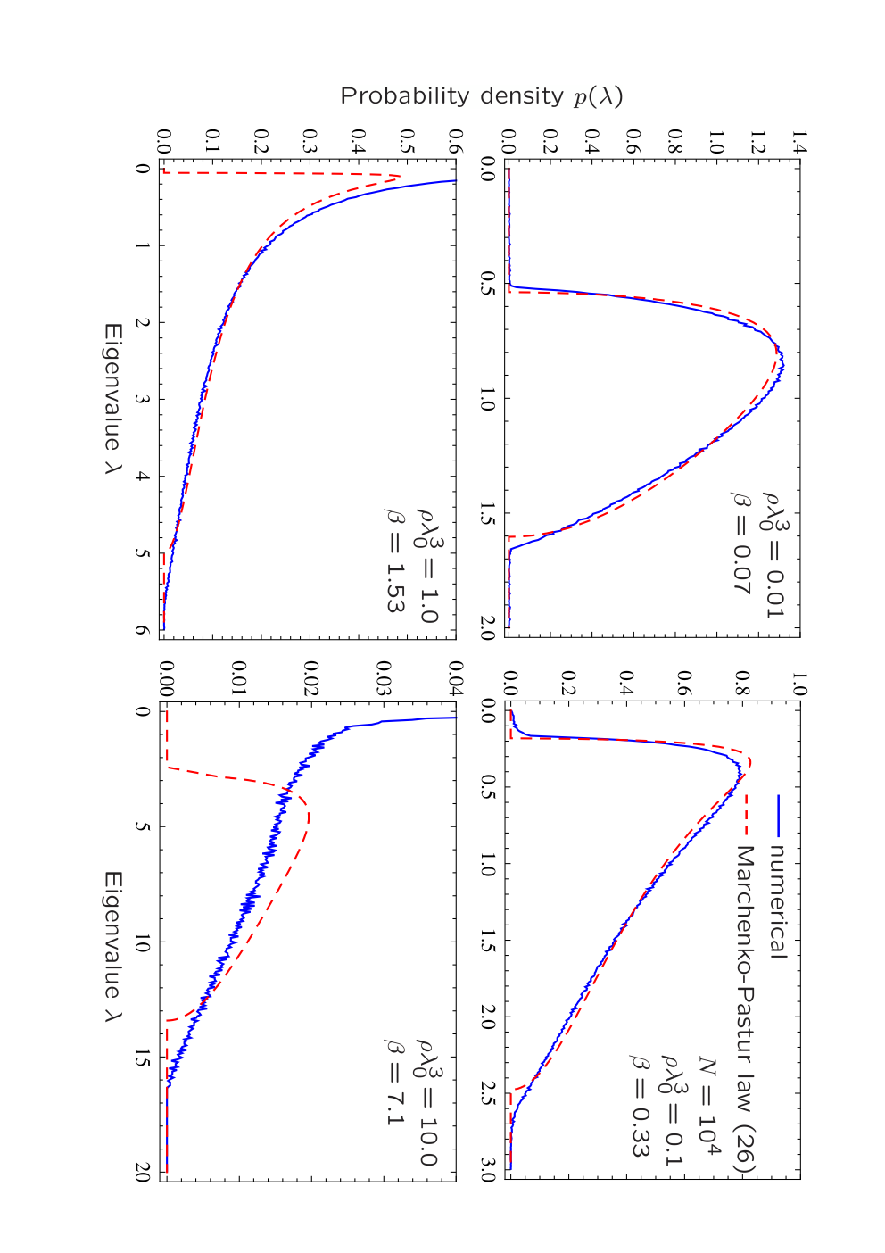
In figure 2 we present a comparison of (14z) with the results of direct numerical simulations. The latter amount to generate $N$ random points $\mathbf{r}_{i}$ inside a three-dimensional cube, to use these points to define a random $N\times N$ matrix ${\hat{S}}$ according to (14u), and to diagonalize ${\hat{S}}$ using the standard software package LAPACK [32]. The procedure is repeated several times and a histogram of all eigenvalues $\lambda$ is created. This histogram approximates the eigenvalue distribution $p(\lambda)$. As we see from figure 2, the agreement between numerical results and the Marchenko-Pastur law (14z) is good for $\beta<1$ but (14z) fails to describe $p(\lambda)$ when $\beta$ becomes larger than unity. The reason for this is easy to understand if we go back to (14v), (14w) and (14x). Indeed, when we approximate the result of integration in (14v) by (14x), we reduce the infinite-size matrix ${\hat{T}}$ to a matrix of finite size $M\times M$. By definition, the rank of the latter matrix is inferior or equal to $M$. The rank of ${\hat{S}}={\hat{H}}{\hat{T}}{\hat{H}}^{\dagger}$ cannot be larger than the rank of ${\hat{T}}$ and hence is also bounded by $M$ from above when we use (14x). When $\beta>1$, implying $M<N$, the representation (4) only gives us access to $M$ of $N$ eigenvalues of ${\hat{S}}$, which is not sufficient to reconstruct the probability density $p(\lambda)$. In order to access the regime of $\beta>1$ one needs to find a better approximation to (14v) than (14x).

Note that the eigenvalue distribution of the matrix ${\hat{S}}$ has been studied numerically by Akkermans et al. in the context of light propagation in atomic gases (see figure 1 of [18]) without proposing any analytical approximation to it. The parameter $\beta\sim N/(k_{0}L)^{2}$ has been introduced in that work as a ratio of the number of atoms $N$ to the number of transverse optical modes $N_{\perp}\propto(k_{0}L)^{2}$. The same parameter appeared in [14, 15, 16, 17] as a superradiant decay rate in a cold atomic gas. Hence the results of this section complement and extend the works [14, 15, 16, 17, 18].

Let us now consider an Euclidean random matrix with elements defined using the cardinal cosine (cosc) function:

The prefactor $1-\delta_{ij}$ allows us to deal with the divergence of the function $\cos(x)/x$ for $x\rightarrow 0$. However, in the beginning of our analysis we will ignore this prefactor and will use $C_{ij}=\cos(k_{0}|\mathbf{r}_{i}-\mathbf{r}_{j}|)/k_{0}|\mathbf{r}_{i}-\mathbf{r}_{j}|$ for all $i,j$ (the diagonal elements of ${\hat{C}}$ are thus infinite). Proceeding as in the previous section, we find

under the same approximations as in (14w) (i.e., we extended integration over $\Delta\mathbf{r}$ to the whole space). The matrix ${\hat{T}}$ defined by (14ae) has infinite size.

The divergence of (14ae) for $q_{m}\rightarrow k_{0}$ can be traced back to the neglect of the finiteness of the volume $V$ when extending integration over $\Delta\mathbf{r}$ to the whole space. Taking into account the fact that $\Delta r$ cannot exceed a maximum value of the order of $L$, the divergence is regularized and the resulting $T_{mn}$ changes sign rapidly but continuously in a strip of width $\sim 1/L$ around $q_{m}=k_{0}$. In the following, we will neglect the contribution of $\mathbf{q}_{m}$’s inside the spherical shell corresponding to this strip because (i) the shell has small thickness in the limit of $k_{0}L\gg 1$ that we are interested in and (ii) $\mathbf{q}_{m}$’s situated symmetrically with respect to the surface $q_{m}=k_{0}$ yield contributions of roughly equal magnitudes but opposite signs which approximately cancel. More precisely, we will exclude a shell of thickness $2\pi\alpha^{\prime}/L$ around $q_{m}=k_{0}$ and will use (14ae) outside this shell [see figure 1(b)]. The numerical constant $\alpha^{\prime}\sim 1$ will be fixed later. The matrix ${\hat{C}}$ therefore takes the form:

Here the first term describes the contribution of $q_{m}<k_{0}-\alpha^{\prime}\pi/L$ with $T^{(1)}_{mn}=4\pi N/[k_{0}V(k_{0}^{2}-q_{m}^{2})]\delta_{mn}$. The matrix ${\hat{T}}^{(1)}$ is a diagonal square matrix of size $M_{1}\simeq(4\pi/3)(k_{0}-\alpha^{\prime}\pi/L)^{3}(L/2\pi)^{3}$ obtained by dividing the volume of a sphere of radius $k_{0}-\alpha^{\prime}\pi/L$ [region 1 corresponding to the inner sphere in figure 1(b)] by the volume $(2\pi/L)^{3}$ associated with a single mode. The second term in (14af) corresponds to $q_{m}>k_{0}+\alpha^{\prime}\pi/L$ [region 3 in figure 1(b)]. The matrix ${\hat{T}}^{(3)}$ is, again, diagonal, with elements $T^{(3)}_{mn}=4\pi N/[k_{0}V(q_{m}^{2}-k_{0}^{2})]\delta_{mn}$ but, in contrast to ${\hat{T}}^{(1)}$, has infinite size. We will treat this matrix as a finite-size matrix of size $M_{3}\simeq(4\pi/3)[q_{\mathrm{max}}^{3}-(k_{0}+\alpha^{\prime}\pi/L)^{3}](L/2\pi)^{3}$, corresponding to taking into account only $q_{m}\leq q_{\mathrm{max}}$. The limit of $q_{\mathrm{max}}\rightarrow\infty$ will be taken at the end. The minus sign in front of the first term in (14af) was introduced to work with a positive-definite matrix ${\hat{T}}^{(1)}$.

The Green’s function of the matrix ${\hat{T}}^{(1)}$ is

where the wavelength $\lambda_{0}=2\pi/k_{0}$ and $\rho\lambda_{0}^{3}$ is the average number of points $\mathbf{r}_{i}$ per wavelength cube. The last line of this equation was obtained in the limit of $k_{0}L\gg 1$ by approximately replacing the summation over a set of discrete wavevectors $\mathbf{q}_{m}$ by an integration over $\boldsymbol{\kappa}=\mathbf{q}_{m}/k_{0}$. The integral in (14ag) can be evaluated yielding

A similar calculation can be performed for the Green’s function of ${\hat{T}}^{(3)}$ except that the integration in (14ag) extends from $1+\alpha^{\prime}\pi/k_{0}L$ to $\kappa_{\mathrm{max}}$, $M_{1}$ is replaced by $M_{3}$, and $1-\kappa^{2}$ in the integrand of (14ag) — by $\kappa^{2}-1$. We find

Because the two terms in (14af) correspond to contributions of different parts of $\mathbf{q}$-space, they are asymptotically free and hence the Blue function of their sum (i.e. of the matrix ${\hat{C}}$) can be found as a sum of their respective Blue functions. The Blue functions of ${\hat{H}}^{(1)}{\hat{T}}^{(1)}{\hat{H}}^{(1)\dagger}$ and ${\hat{H}}^{(3)}{\hat{T}}^{(3)}{\hat{H}}^{(3)\dagger}$ are found using (14s), whereas the Blue function of $-{\hat{H}}^{(1)}{\hat{T}}^{(1)}{\hat{H}}^{(1)\dagger}$ is equal to $-B_{{\hat{H}}^{(1)}{\hat{T}}^{(1)}{\hat{H}}^{(1)\dagger}}(-z)$. The Blue function of the sum ${\hat{C}}=-{\hat{H}}^{(1)}{\hat{T}}^{(1)}{\hat{H}}^{(1)\dagger}+{\hat{H}}^{(3)}{\hat{T}}^{(3)}{\hat{H}}^{(3)\dagger}$ is a sum of individual Blue functions, minus $1/z$:

where $\beta^{\prime}=\pi N/\alpha^{\prime}(k_{0}L)^{2}$.

The final step consists in taking the limit $\kappa_{\mathrm{max}}\rightarrow\infty$. We now recall that up to now we ignored the fact that the matrix ${\hat{C}}$ had zero diagonal elements $C_{ii}=0$. Instead, we considered a matrix with infinitely large diagonal elements. Such a matrix naturally has infinite eigenvalues and to go back to the case of $C_{ii}=0$ we have to shift the eigenvalues to the left. To determine the exact shift, we compute the average of $\lambda$ from (14aj) using (14q) and subtract it from (14aj) because we know that for the matrix ${\hat{C}}$ defined by (14ad), $\langle\lambda\rangle=(1/N)\langle\Tr{\hat{C}}\rangle=0$ exactly ⁴⁴ 4 Subtracting a constant from the Blue function $B(z)$ results in shifting the eigenvalue distribution $p(\lambda)$.. We then compute the second moment $\langle\lambda^{2}\rangle$ and require that its value in the limit of $\rho\lambda_{0}^{3}/\beta^{\prime}\propto 1/k_{0}L\rightarrow 0$ is equal to $\beta$ defined by (14ac). This fixes $\beta^{\prime}=(\pi^{2}/4)\beta$ corresponding to $\alpha^{\prime}\simeq 0.45$. The final expression for the Blue function of ${\hat{C}}$ is

References

- [1] Mehta M L 1991 Random Matrices (New York: Academic)
- [2] Beenakker C W J 1997 Rev. Mod. Phys. 69 731
- [3] Fyodorov Y V and Sommers H J 1997 J. Math. Phys. 38 1918
- [4] Guhr T, Müller-Groeling A, Weidenmüller H A 1998 Phys. Rep. 299 189
- [5] Mézard M, Parisi G and Zee A 1999 Nucl. Phys. B 559 689
- [6] Parisi G 2006 in Applications of Random Matrices in Physics. NATO Science Series, Series II: Mathematics, Physics and Chemistry 221 219
- [7] Grigera T S, Martin-Mayor V, Parisi G and Verrocchio P 2003 Nature 422 289
- [8] Amir A, Oreg Y and Imry Y 2010 Phys. Rev. Lett. 105 070601
- [9] Rusek M, Orlowski A and Mostowski J 1996 Phys. Rev. E 53 4122
- [10] Rusek M, Mostowski J and Orlowski A 2000 Phys. Rev. A 61 022704
- [11] Pinheiro F A, Rusek M, Orlowski A and Van Tiggelen B A 2004 Phys. Rev. E 69 026605
- [12] Antezza M, Castin Y and Hutchinson D 2010 Phys. Rev. A 82 043602
- [13] Ernst V 1969 Z. Phys. 218 111
- [14] Svidzinsky A and Chang J T 2008 Phys. Rev. A 77 043833
- [15] Scully M O 2009 Phys. Rev. Lett. 102 143601
- [16] Svidzinsky A A and Scully M O 2009 Opt. Commun. 282 2894
- [17] Svidzinsky A A, Chang J T and Scully M O 2010 Phys. Rev. A 81 053821
- [18] Akkermans E, Gero A and Kaiser R 2008 Phys. Rev. Lett. 101 103602
- [19] Pinheiro F A and Sampaio L C 2006 Phys. Rev. A 73 013826
- [20] Goetschy A and Skipetrov S E (in preparation)
- [21] Grémaud B and Wellens T 2010 Phys. Rev. Lett. 104 133901
- [22] Labeyrie G, De Tomasi F, Bernard J C, Müller C A, Miniatura C and Kaiser R 1999 Phys. Rev. Lett. 83 5266
- [23] Labeyrie G, Vaujour E, Müller C A, Delande D, Miniatura C, Wilkowski D and Kaiser R 2003 Phys. Rev. Lett. 91 223904
- [24] Anderson P W 1958 Phys. Rev. 109 1492
- [25] Lagendijk A, Van Tiggelen B A and Wiersma D S 2009 Physics Today 62(8) 24
- [26] Special Issue: 50 Years of Anderson Localization 2010 Int. J. Mod. Phys. B 24 1501
- [27] Voiculescu D V, Dykema K J and Nica A 1992 Free Random Variables (Province, RI: American Mathematical Society)
- [28] Tulino A M and Verdú S 2004 Random Matrix Theory and Wireless Communications (Delft: Now Publishers)
- [29] Janik R A, Nowak M A, Papp G, Wambach J and Zahed I 1997 Phys. Rev. E 55 4100
- [30] Marčenko V A and Pastur L A 1967 Mat. Sbornik (USSR) 1 457
- [31] Sengupta A M and Mitra P P 1999 Phys. Rev. E 60 3389
- [32] http://www.netlib.org/lapack/
- [33] Zee A 1996 Nucl. Phys. B 474 726.
- [34] Jarosz A and Nowak M A 2006 J. Phys. A: Math. Gen. 39 10107
- [35] Chalker J T and Mehlig B 1998 Phys. Rev. Lett. 81 3367
- [36] Haake F, Izrailev F, Lehmann N, Saher D, Sommers H J 1992 Z. Phys. B 88 359
- [37] Lehmann N, Saher D, Sokolov V V, Sommers H J 1995 Nucl. Phys. A 582 223
- [38] Feinberg J, Zee A 1997 Nucl. Phys. B 504 579
- [39] Feinberg J 2006 J. Phys. A: Math. Gen. 39 10029
- [40] Kottos T 2005 . J. Phys. A: Math. Gen. 38 10761
- [41] Cao H 2003 Waves in Random Media 13 R1
- [42] Cao H 2005 . J. Phys. A: Math. Gen. 38 10497
- [43] Wiersma D S 2008 Nat. Phys. 4 359