跳到论文正文
W Papers独立论文阅读器 arXiv:1007.1334 论文正文 计算阅读时间 · 0%
引用这篇论文根据当前论文元数据生成,正式投稿前建议核对。


License: arXiv.org perpetual non-exclusive license
arXiv:1007.1334v1 [math.OC] 08 Jul 2010

Stabilization for an ensemble of half-spin systemsThanks: KB and PR were partially supported by the “Agence Nationale de la Recherche” (ANR), Projet Blanc C-QUID number BLAN-3-139579. PSPS was partially supported by CNPq – Conselho Nacional de Desenvolvimento Cientifico e Tecnologico – Brazil, under grant 308465/2006-7.

Karine Beauchard ††thanks: CMLA, ENS Cachan, CNRS, UniverSud, 61, avenue du Président Wilson, F-94230 Cachan, FRANCE. Email: karine.beauchard@cmla.ens-cachan.fr    Paulo Sérgio Pereira da Silva ††thanks: Escola Politécnica da USP - PTC Cep 05508-900 – São Paulo – SP – BRAZIL.Email: paulo@lac.usp.br    Pierre Rouchon ††thanks: Mines ParisTech, Centre Automatique et Systèmes, Unité Mathématiques et Systèmes, 60 Bd Saint-Michel, 75272 Paris cedex 06, FRANCE. Email: pierre.rouchon@mines-paristech.fr
Abstract

Feedback stabilization of an ensemble of non interacting half spins described by Bloch equations is considered. This system may be seen as a prototype for infinite dimensional systems with continuous spectrum. We propose an explicit feedback law that stabilizes asymptotically the system around a uniform state of spin +1/2 or -1/2. The proof of the convergence is done locally around the equilibrium in the H1H^{1} topology. This local convergence is shown to be a weak asymptotic convergence for the H1H^{1} topology and thus a strong convergence for the C0C^{0} topology. The proof relies on an adaptation of the LaSalle invariance principle to infinite dimensional systems. Numerical simulations illustrate the efficiency of these feedback laws, even for initial conditions far from the equilibrium

Keywords:

Nonlinear systems, Lyapunov stabilization, LaSalle invariance, ensemble controllability, infinite dimensional systems.

1 Introduction

1.1 Infinite dimensional systems with continuous spectra

Most controllability results available for infinite dimensional bilinear systems are related to systems with discrete spectra (see for instance, [2] for exact controllability results and [5, 13] for approximate controllability results). As far as we know, very few controllability studies consider systems admitting a continuous part in their spectra.

In [11] an approximate controllability result is given for a system with mixed discrete/continuous spectrum: the Schrödinger partial differential equation of a quantum particle in an N-dimensional decaying potential is shown to be approximately controllable (in infinite time) to the ground bounded state when the initial state is a linear superposition of bounded states.

In [9, 10] a controllability notion, called ensemble controllability, is introduced and discussed for quantum systems described by a family of ordinary differential equations (Bloch equations) depending continuously on a finite number of scalar parameters and with a finite number of control inputs. Ensemble controllability means that it is possible to find open-loop controls that compensate for the dispersion in these scalar parameters: the goal is to simultaneously steer a continuum of systems between states of interest with the same control input. Such continuous family of ordinary differential systems sharing the same control inputs can be seen as the prototype of infinite dimensional systems with purely continuous spectra.

The article [10] highlights the role of Lie algebras and non-commutativity in the design of a compensating control sequence and consequently in the characterization of ensemble controllability. In [3], this analysis is completed by functional analysis methods developed for infinite dimensional systems governed by partial differential equations (see, e.g., [8] for samples of these methods). Several mathematical answers are given, with discrimination between approximate and exact controllability, and finite time and infinite time controllability, for the Bloch equation. In particular, it is proved that a priori bounded L2L^{2}-controls are not sufficient to achieve exact controllability, but unbounded controls (containing, for example sums of Dirac masses) allow to recover controllability. For example, it is proved in [3] that the Bloch equation is approximately controllable to e3e_{3}, in H1H^{1}, in finite time, with unbounded controls. The authors also propose explicit open loop (unbounded) controls for the local exact controllability to e3e_{3} in infinite time.

The goal of this article is to investigate feedback stabilization of such specific infinite dimensional systems with continuous spectra. As in [11], the feedback design is based on a Lyapunov function closely related to the norm of the state space, a Banach space.

1.2 The studied model

We consider here an ensemble of non interacting half-spins in a static field (0,0,B0)T(0,0,B_{0})^{T} in ℝ3\mathbb{R}^{3}, subject to a transverse radio frequency field (u~​(t),v~​(t),0)T(\tilde{u}(t),\tilde{v}(t),0)^{T} in ℝ3\mathbb{R}^{3} (the control input). The ensemble of half-spins is described by the magnetization vector M∈ℝ3M\in\mathbb{R}^{3} depending on time tt but also on the Larmor frequency ω=−γ​B0\omega=-\gamma B_{0} (γ\gamma is the gyromagnetic ratio). It obeys to the Bloch equation:

∂M∂t​(t,ω)=(u~​(t)​e1+v~​(t)​e2+ω​e3)×M⁡(t,ω),\frac{\partial M}{\partial t}(t,\omega)=(\tilde{u}(t)e_{1}+\tilde{v}(t)e_{2}+\omega e_{3})\times M(t,\omega), (1)

where −∞<ω∗<ω∗<+∞-\infty<\omega_{*}<\omega^{*}<+\infty, ω∈(ω∗,ω∗)\omega\in(\omega_{*},\omega^{*}), (e1,e2,e3)(e_{1},e_{2},e_{3}) is the canonical basis of ℝ3\mathbb{R}^{3}, ×\times denotes the vector product on ℝ3\mathbb{R}^{3}. The equation (1) is an infinite dimensional bilinear control system in which

  • —

    the state is the function MM, with, for every ω∈(ω∗,ω∗)\omega\in(\omega_{*},\omega^{*}), M⁡(t,ω)∈𝕊2M(t,\omega)\in\mathbb{S}^{2}, the unit sphere of ℝ3\mathbb{R}^{3},

  • —

    the two control inputs u~\tilde{u} and v~\tilde{v} are real valued.

It must be stressed that u~​(t)\tilde{u}(t) and v~​(t)\tilde{v}(t) are common controls for all the members of the ensemble, and they cannot depend on ω\omega. In coordinates M=(x,y,z)M=(x,y,z), the Bloch equation may be written

{x˙=−ω​y+v~​z,y˙=ω​x−u~​z,z˙=−v~​x+u~​y,\left\{\begin{array}[]{rcl}\dot{x}&=&-\omega y+\tilde{v}z,\\ \dot{y}&=&\omega x-\tilde{u}z,\\ \dot{z}&=&-\tilde{v}x+\tilde{u}y,\end{array}\right. (2)

where x˙\dot{x} stands for ∂x/∂t\partial x/\partial t.

Now, let us precise the definition of a solution associated to Dirac controls. When u~,v~∈Ll​o​c1​(ℝ)\tilde{u},\tilde{v}\in L^{1}_{loc}(\mathbb{R}), then, for every initial condition M0∈L2​((ω∗,ω∗),ℝ3)M_{0}\in L^{2}((\omega_{*},\omega^{*}),\mathbb{R}^{3}), the equation (1) has a weak solution in the usual sense: M∈C0([0,+∞),L2((ω∗,ω∗),ℝ3))M\in C^{0}([0,+\infty),L^{2}((\omega_{*},\omega^{*}),\mathbb{R}^{3})). Let us give the definition of a solution associated to a Dirac control. In the sequel δa​(t)\delta_{a}(t) stands for the Dirac function δ⁡(t−a)\delta(t-a). If u~=α​δa​(t)+u♯\tilde{u}=\alpha\delta_{a}(t)+u_{\sharp} and v~=v♯\tilde{v}=v_{\sharp} where u♯,v♯∈Ll​o​c1​(ℝ)u_{\sharp},v_{\sharp}\in L^{1}_{loc}(\mathbb{R}), α>0\alpha>0 and a∈(0,+∞)a\in(0,+\infty), then the solution is the classical solution on [0,a)[0,a) and (a,+∞)(a,+\infty), it is discontinuous at the point aa, with the explicit discontinuity

M⁡(a+,ω)=(1000cos⁡(α)−sin⁡(α)0sin⁡(α)cos⁡(α))​M​(a−,ω).M(a^{+},\omega)=\left(\begin{array}[]{ccc}1&0&0\\ 0&\cos(\alpha)&-\sin(\alpha)\\ 0&\sin(\alpha)&\cos(\alpha)\end{array}\right)M(a^{-},\omega).

This definition corresponds to the limit, as ϵ→0+\epsilon\rightarrow 0^{+} of solutions associated to u~​(t)=(α/ϵ)​1[a,a+ϵ]​(t)\tilde{u}(t)=(\alpha/\epsilon)1_{[a,a+\epsilon]}(t).

Formally, the spectrum of the operator AA defined by

(A​M)​(ω):=ω​e3×M⁡(ω)(AM)(\omega):=\omega e_{3}\times M(\omega)

is −i⁡(ω∗,ω∗)∪i⁡(ω∗,ω∗)-i(\omega_{*},\omega^{*})\cup i(\omega_{*},\omega^{*}): for every ω♯∈(ω∗,ω∗)\omega_{\sharp}\in(\omega_{*},\omega^{*}), the eigenvector associated to ±i​ω♯\pm i\omega_{\sharp} is (1,∓i,0)T​δω♯​(ω)(1,\mp i,0)^{T}\delta_{\omega_{\sharp}}(\omega). Thus the Bloch equation (1) is a prototype of infinite dimensional system with continuous spectrum.

1.3 Outline

The goal of this article it to propose a first answer to the following question.

Local Stabilization Problem. Define an explicit control law (u~,v~)=(u~​(t,M),v~​(t,M))(\tilde{u},\tilde{v})=(\tilde{u}(t,M),\tilde{v}(t,M)) and a neighborhood UU of −e3-e_{3} (in some space of functions (ω∗,ω∗)→𝕊2(\omega_{*},\omega^{*})\rightarrow{\mathbb{S}}^{2} to be determined) such that, given any initial condition M0∈UM^{0}\in U, the solution of the closed loop system is defined for every t∈[0,+∞)t\in[0,+\infty), is unique and converges to −e3-e_{3}, when t→+∞t\rightarrow+\infty, uniformly with respect to ω∈(ω∗,ω∗)\omega\in(\omega_{*},\omega^{*}).

Section 2 is devoted to control design and closed-loop simulations: the feedback law is the sum of a Dirac comb and a time-periodic feedback law based on a Lyapunov function; Proposition 1 proved in Appendix A guarantees that the closed-loop initial value problem is always well defined; simulations illustrate the convergence rates observed for an initial state formed by a quarter of the equator on the Bloch sphere. In section 3 we state and prove the main convergence result, Theorem 1: the closed-loop convergence towards the constant profile M⁡(ω)=−e3M(\omega)=-e_{3} is shown to be local and weak for the H1H^{1} topology on MM. The obstruction to global stabilization is also discussed: it is based on an explicit description of the Lasalle invariant set. Some concluding remarks are gathered in section 4.

2 Lyapunov H1H^{1} approach

2.1 The impulse-train control

It is proved in [3] that controls containing sums of Dirac masses are crucial to achieve the controllability of the Bloch equation. In view of the controls used in this reference, it is natural to consider a control with the following “impulse-train” structure

u~=u+∑k=1+∞π​δk​T​(t),v~=(−1)E⁡(tT)​v\tilde{u}=u+\sum_{k=1}^{+\infty}\pi\penalty\ \delta_{k\!T}(t),\quad\tilde{v}=(-1)^{E\left(\frac{t}{T}\right)}v (3)

for some period T>0T>0, which is fixed in all the article (E⁡(γ)E\left(\gamma\right) denotes the integer part of the real number γ\gamma). The new controls uu and vv belong to Ll​o​c1​(ℝ)L^{1}_{loc}(\mathbb{R}). Then, after each impulse that is applied at time t=k​Tt=kT, xx remains unchanged, but yy and zz are moved to their opposites, that is

(x,y,z)​(k​T+)=(x,−y,−z)​(k​T−).(x,y,z)(kT^{+})=(x,-y,-z)(kT^{-}).

The resulting state diffeomorphism

(x,y,z)↦(𝒳=x,𝒴=−y,𝒵=−z)(x,y,z)\mapsto(\mathcal{X}=x,\mathcal{Y}=-y,\mathcal{Z}=-z) (4)

transforms (2) into

𝒳˙​(t)\displaystyle\dot{\mathcal{X}}(t) =\displaystyle= ω​𝒴​(t)−v~​(t)​𝒵​(t),\displaystyle\omega\mathcal{Y}(t)-\tilde{v}(t)\mathcal{Z}(t),
𝒴˙​(t)\displaystyle\dot{\mathcal{Y}}(t) =\displaystyle= −ω​𝒳​(t)−u~​𝒵​(t),\displaystyle-\omega\mathcal{X}(t)-\tilde{u}\mathcal{Z}(t),
𝒵˙​(t)\displaystyle\dot{\mathcal{Z}}(t) =\displaystyle= v~​(t)​𝒳​(t)+u~​(t)​𝒴​(t).\displaystyle\tilde{v}(t)\mathcal{X}(t)+\tilde{u}(t)\mathcal{Y}(t).

Let ς=(−1)E⁡(tT)\varsigma=(-1)^{E\left(\frac{t}{T}\right)}. Considering the following change of variables

(x,y,z)​(t,ω)↦(x⁡(t,ω),ζ⁡(t)​y​(t,ω),ζ⁡(t)​z​(t,ω))(x,y,z)(t,\omega)\mapsto\Big(x(t,\omega),\zeta(t)y(t,\omega),\zeta(t)z(t,\omega)\Big)

one gets the following dynamics

{x˙=−ς​ω​y+v​z,y˙=ς​ω​x−u​z,z˙=−v​x+u​y,\left\{\begin{array}[]{l}\dot{x}=-\varsigma\omega y+vz,\\ \dot{y}=\varsigma\omega x-uz,\\ \dot{z}=-vx+uy,\end{array}\right. (5)

with the new control (u,v)(u,v) as in (3). It is as if, between [k​T,(k+1)​T][kT,(k+1)T] and [(k+1)​T,(k+2)​T][(k+1)T,(k+2)T], one is changing the sign of ω\omega, but the solution, after the identification (4), remains continuous in tt (but not differentiable in tt at the instants t=k​T,k∈ℕt=kT,k\in{\mathbb{N}}). In other words, the application of the impulses at t=k​Tt=kT changes the sense of rotation of the null input solution. One would expect that this impulse-train control is reducing the average dispersion of the solution. Roughly speaking, the dispersion observed for the open-loop system (2) with (u~,v~)(\tilde{u},\tilde{v}) as input is strongly reduced and almost canceled for the open-loop system (5) with (u,v)(u,v) as input.

2.2 Heuristics of the Lyapunov-like control

Now let Z⁡(t,ω)Z(t,\omega) and Ω⁡(t)\Omega(t) defined by

Z=x+i​y,Ω=v−i​uZ=x+iy,\quad\Omega=v-iu

where x,y,zx,y,z refer to the transformed dynamics (5). Then one may write (5) in the form

{Z˙​(t,ω)=i​ς​(t)​ω​Z​(t,ω)+Ω⁡(t)​z​(t,ω),z˙​(t,ω)=−ℜ⁡[Ω⁡(t)​Z⁡(t,ω)¯],\left\{\begin{array}[]{rcl}\dot{Z}(t,\omega)&=&i\varsigma(t)\omega Z(t,\omega)+\Omega(t)z(t,\omega),\\ \dot{z}(t,\omega)&=&-\Re\left[\Omega(t)\overline{Z(t,\omega)}\right],\end{array}\right.

where ℜ⁡(ξ)\Re(\xi) (resp. ξ¯\overline{\xi}) denotes the real part (resp. the complex conjugate number) of a complex number ξ∈ℂ\xi\in\mathbb{C}. The following transformation

Z~(t,ω)=Z(t,ω)e−iω∫0tς(τ)dτ\tilde{Z}(t,\omega)=Z(t,\omega)e^{-i\omega\int_{0}^{t}\varsigma(\tau)d\tau}

converts the system into the driftless form

{Z˙​(t,ω)=Ω(t)z(t,ω)e−iω∫0tς,z˙​(t,ω)=−ℜ[Ω(t)Z⁡(t,ω)¯e−iω∫0tς],\left\{\begin{array}[]{rcl}\dot{Z}(t,\omega)&=&\Omega(t)z(t,\omega)e^{-i\omega\int_{0}^{t}\varsigma},\\ \dot{z}(t,\omega)&=&-\Re\left[\Omega(t)\overline{Z(t,\omega)}e^{-i\omega\int_{0}^{t}\varsigma}\right],\end{array}\right. (6)

where, for notation simplicity, one lets Z⁡(t,ω)Z(t,\omega) stand for Z~​(t,ω)\tilde{Z}(t,\omega), and one lets ∫0tς\int_{0}^{t}\varsigma stand for ∫0tς⁡(τ)​𝑑τ\int_{0}^{t}\varsigma(\tau)d\tau.

For the moment one shall assume that the input Ω⁡(t)\Omega(t) will be chosen in such a way that the solution (Z⁡(t,ω),z⁡(t,ω))(Z(t,\omega),z(t,\omega)) of (6) does exist, it is unique and it is regular enough in a way that one may consider that the derivatives Z′​(t,ω)=∂Z∂ω​(t,ω)Z^{\prime}(t,\omega)=\frac{\partial{Z}}{\partial\omega}(t,\omega) and z′​(t,ω)=∂z∂ω​(t,ω)z^{\prime}(t,\omega)=\frac{\partial{z}}{\partial\omega}(t,\omega) exist almost everywhere and they are solutions of the differential equation that is obtained by differentiation of (6) with respect to ω\omega, namely

{Z˙′=Ω{[z′−i(∫0tς)z]e−iω∫0tς},z˙′=−ℜ{Ω[Z¯′−i(∫0tς)Z¯]e−iω∫0tς},\left\{\begin{array}[]{l}\dot{Z}^{\prime}=\Omega\left\{\left[z^{\prime}-i\left(\int_{0}^{t}\varsigma\right)z\right]e^{-i\omega\int_{0}^{t}\varsigma}\right\},\\ \dot{z}^{\prime}=-\Re\left\{\Omega\left[\overline{Z}^{\prime}-i\left(\int_{0}^{t}\varsigma\right)\overline{Z}\right]e^{-i\omega\int_{0}^{t}\varsigma}\right\},\end{array}\right. (7)

where Z˙′\dot{Z}^{\prime} stands for ∂∂t​Z′\frac{\partial}{\partial t}{Z}^{\prime}, and z˙′\dot{z}^{\prime} stands for ∂∂t​z′\frac{\partial}{\partial t}{z}^{\prime}.

Now consider the following Lyapunov-like functional:

ℒ=12​∫ω∗ω∗{|Z′|2+(z′)2+2​G​(z+1)}​𝑑ω\penalty\ \mathcal{L}=\frac{1}{2}\int\limits_{\omega_{*}}^{\omega^{*}}\left\{|Z^{\prime}|^{2}+(z^{\prime})^{2}+2G(z+1)\right\}d\omega (8)

where GG is a positive real number and Z⁡(t,ω),Z′​(t,ω)Z(t,\omega),Z^{\prime}(t,\omega) and z′​(t,ω)z^{\prime}(t,\omega) refer to the solutions respectively of (6) and (7). One may write

dd​t​ℒ​(t)=ℜ⁡(∫ω∗ω∗{Z¯′​Z˙′+z′​z˙′+G​z˙}​𝑑ω){\frac{d}{dt}}\mathcal{L}(t)=\Re\left(\int\limits_{\omega_{*}}^{\omega^{*}}\left\{\bar{Z}^{\prime}\dot{Z}^{\prime}+z^{\prime}\dot{z}^{\prime}+G\dot{z}\right\}d\omega\right) (9)

and so, taking into account (6) and (7), the fact that Ω⁡(t)\Omega(t) does not depend on ω\omega, one gets

dd​t​ℒ​(t)=ℜ⁡[Ω⁡(t)​H​(t)]{\frac{d}{dt}}\mathcal{L}(t)=\Re\left[\Omega(t)H(t)\right] (10)

where

H(t):=∫ω∗ω∗{i(∫0tς)(Z¯z′−Z¯′z)−GZ¯}e−iω∫0tςdω.H(t):=\int\limits_{\omega_{*}}^{\omega^{*}}\Big\{i\left(\int\limits_{0}^{t}\varsigma\right)\left(\bar{Z}z^{\prime}-\bar{Z}^{\prime}z\right)-G\bar{Z}\Big\}e^{-i\omega\int_{0}^{t}\varsigma}d\omega.

Hence one may take Ω⁡(t)=−Kp​H¯​(t)\Omega(t)=-K_{p}\bar{H}(t), where KpK_{p} is a positive real number, obtaining

Ω⁡(t)=Kp​∫ω∗ω∗{i⁡(∫0tς)​(Z​z′−Z′​z)+G​Z}​ei​ω​∫0tς​𝑑ω.\Omega(t)=K_{p}\int\limits_{\omega_{*}}^{\omega^{*}}\Big\{i\left(\int\limits_{0}^{t}\varsigma\right)\left(Zz^{\prime}-{Z}^{\prime}z\right)+GZ\Big\}e^{i\omega\int_{0}^{t}\varsigma}d\omega. (11)

It follows that

d​ℒd​t​(t)=−1Kp​|Ω⁡(t)|2.\frac{d\mathcal{L}}{dt}(t)=-\frac{1}{K_{p}}|\Omega(t)|^{2}.

Consider the system (6) in closed loop with the control law (11), thereby called by closed loop system. The state space of this system is H1​((ω∗,ω∗),ℝ3)H^{1}((\omega_{*},\omega^{*}),{\mathbb{R}}^{3}), which is the set of functions f∈L2​(ω∗,ω∗)f\in L^{2}(\omega_{*},\omega^{*}) such that the distributional derivative f′f^{\prime} belongs to L2​(ω∗,ω∗)L^{2}(\omega_{*},\omega^{*}). This space, equipped with the norm

‖f‖H1:=(∫ω∗ω∗|f′​(ω)|2+|f⁡(ω)|2​𝑑ω)1/2\|f\|_{H^{1}}:=\left(\int\limits_{\omega_{*}}^{\omega^{*}}|f^{\prime}(\omega)|^{2}+|f(\omega)|^{2}d\omega\right)^{1/2}

is a Banach space. In other words, closed-loop system (6)-(11) may be considered to be a differential equation of the form

{M˙​(t)=F⁡(t,M⁡(t))M⁡(0)=M0∈H1​((ω∗,ω∗),𝕊2)\left\{\begin{array}[]{lll}\dot{M}(t)&=&F(t,M(t))\\ M(0)&=&M^{0}\in H^{1}((\omega_{*},\omega^{*}),{\mathbb{S}}^{2})\end{array}\right.

where F⁡(t,M)F(t,M) is a continuous map

F:ℝ×H1​((ω∗,ω∗),ℝ3)→H1​((ω∗,ω∗),ℝ3).F:{\mathbb{R}}\times H^{1}((\omega_{*},\omega^{*}),{\mathbb{R}}^{3})\rightarrow H^{1}((\omega_{*},\omega^{*}),{\mathbb{R}}^{3}).

Moreover, FF is locally integrable (Ll​o​c1L^{1}_{loc}) and periodic in tt and locally Lipschitz in MM. Using the same ideas as in the proof of the Cauchy-Lipschitz (Picard-Lindelöf) theorem, we get local (in time) solutions in C0​([0,T],H1)C^{0}([0,T],H^{1}). From the contruction of the feedback law, finite time blow up in H1H^{1} is impossible, thus solutions are global in time. Precisely, we have the following result, whose proof is detailed in Appendix A.

Proposition 1

For every initial condition M0∈H1​((ω∗,ω∗),𝕊2)M^{0}\in H^{1}((\omega_{*},\omega^{*}),{\mathbb{S}}^{2}), the closed loop system (6), (11) has a unique solution M∈Cp​w1​([0,∞),H1​((ω∗,ω∗),𝕊2))M\in C^{1}_{pw}\left([0,\infty),H^{1}\left((\omega_{*},\omega^{*}),\mathbb{S}^{2}\right)\right) such that M⁡(0)=M0M(0)=M^{0}.

In this statement, the space Cp​w1​([0,∞),H1​((ω∗,ω∗),𝕊2))C^{1}_{pw}\left([0,\infty),H^{1}\left((\omega_{*},\omega^{*}),{\mathbb{S}}^{2}\right)\right) is made of functions
M∈C0​([0,∞),H1​((ω∗,ω∗),𝕊2))M\in C^{0}\left([0,\infty),H^{1}\left((\omega_{*},\omega^{*}),{\mathbb{S}}^{2}\right)\right) such that M∈C1​((k​T,(k+1)​T),H1​((ω∗,ω∗),𝕊2))M\in C^{1}((kT,(k+1)T),H^{1}\left((\omega_{*},\omega^{*}),{\mathbb{S}}^{2}\right)), for every k∈ℕk\in\mathbb{N}; their derivative ∂M/∂t\partial M/\partial t is possibly discontinuous at t=k​Tt=kT, but it has finite limits in H1​((ω∗,ω∗),𝕊2)H^{1}\left((\omega_{*},\omega^{*}),\mathbb{S}^{2}\right) when t→(k​T)+t\rightarrow(kT)^{+} and t→(k​T)−t\rightarrow(kT)^{-}.

2.3 Closed-loop simulations

We assume here ω∗=0\omega_{*}=0, ω∗=1\omega^{*}=1 and we solve numerically the TT-periodic system (5) with the TT-periodic feedback law (11) where Z=x+ı​yZ=x+\imath y and Ω=v−ı​u\Omega=v-\imath u. The parameters are T=2​π/(ω∗−ω∗)T=2\pi/(\omega^{*}-\omega_{*}), Kp=1K_{p}=1, G=T2/20G=T^{2}/20. The simulation is for t∈[0,Tf]t\in[0,T_{f}], Tf=20​TT_{f}=20T. The ω\omega-profile [ω∗,ω∗]∋ω↦(x⁡(t,ω),y⁡(t,ω),z⁡(t,ω))[\omega_{*},\omega^{*}]\ni\omega\mapsto(x(t,\omega),y(t,\omega),z(t,\omega)) is discretized {0,…,N}∋k↦(xk​(t),yk​(t),zk​(t))\{0,\ldots,N\}\ni k\mapsto(x_{k}(t),y_{k}(t),z_{k}(t)) with a regular mesh of step ϵN=ω∗−ω∗N\epsilon_{N}=\frac{\omega^{*}-\omega_{*}}{N} and N=100N=100: (xk​(t),yk​(t),zk​(t))(x_{k}(t),y_{k}(t),z_{k}(t)) is then an approximation of (x⁡(t,k​ϵN),y⁡(t,k​ϵN),z⁡(t,k​ϵN))(x(t,k\epsilon_{N}),y(t,k\epsilon_{N}),z(t,k\epsilon_{N})). We have checked that the closed-loop simulations are almost identical for N=100N=100 and N=200N=200. In the feedback law (11), the integral versus ω\omega is computed assuming that (x,y,z)(x,y,z) and (x′,y′,z′)(x^{\prime},y^{\prime},z^{\prime}) are constant over ](k−12)​ϵN,(k+12)​ϵN[](k-\frac{1}{2})\epsilon_{N},(k+\frac{1}{2})\epsilon_{N}[, their values being (xk,yk,zk)(x_{k},y_{k},z_{k}) and (xk+1−xk−12​ϵN,yk+1−yk−12​ϵN,zk+1−zk−12​ϵN)\left(\frac{x_{k+1}-x_{k-1}}{2\epsilon_{N}},\frac{y_{k+1}-y_{k-1}}{2\epsilon_{N}},\frac{z_{k+1}-z_{k-1}}{2\epsilon_{N}}\right). The obtained differential system is of dimension 3​(N+1)3(N+1). It is integrated via an explicit Euler scheme with a step size h=T/800h=T/800. We have tested that h=T/1600h=T/1600 yields to almost the same numerical solution at t=Tf=20​Tt=T_{f}=20T. After each time-step the new values of (xk,yk,zk)(x_{k},y_{k},z_{k}) are normalized to remain in 𝕊2{\mathbb{S}}^{2}.

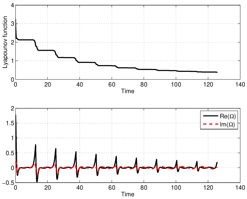
Figures 1 and 2 summarize the main convergence issues when the initial ω\omega-profiles of (x,y,z)∈𝕊2(x,y,z)\in{\mathbb{S}}^{2} are z⁡(0,ω)=0z(0,\omega)=0, x⁡(0,ω)=cos⁡(π2​ω+π4)x(0,\omega)=\cos\left(\tfrac{\pi}{2}\omega+\tfrac{\pi}{4}\right) and y⁡(0,ω)=sin⁡(π2​ω+π4)y(0,\omega)=\sin\left(\tfrac{\pi}{2}\omega+\tfrac{\pi}{4}\right). The convergence speed is rapid at the beginning and tends to decrease at the end. We start with ℒ⁡(0)≈3.24{\mathcal{L}}(0)\approx 3.24 and supω∈[ω∗,ω∗]‖M⁡(0,ω)+e3‖≈1.41\sup_{\omega\in[\omega_{*},\omega^{*}]}\|M(0,\omega)+e_{3}\|\approx 1.41. We get ℒ⁡(20​T)≈0.38{\mathcal{L}}(20T)\approx 0.38 and supω∈[ω∗,ω∗]‖M⁡(20​T,ω)+e3‖≈0.27\sup_{\omega\in[\omega_{*},\omega^{*}]}\|M(20T,\omega)+e_{3}\|\approx 0.27. The control problem is quite hard due to the fact that one has a continuous spectrum, that is, an infinite ensemble of systems with a common control input Ω⁡(t)\Omega(t). Hence, as time increases, the control must fight against the dispersion of the solutions M⁡(t,ω)M(t,\omega) for different values of ω\omega. Simulations (not presented here) on much longer times until 1000​T1000T and with the same initial conditions and parameters always yield to smaller final value for the Lyapunov function: we get ℒ⁡(1000​T)≈0.02{\mathcal{L}}(1000T)\approx 0.02 and supω∈[ω∗,ω∗]‖M⁡(1000​T,ω)+e3‖≈0.04\sup_{\omega\in[\omega_{*},\omega^{*}]}\|M(1000T,\omega)+e_{3}\|\approx 0.04. This is a strong indication of asymptotic converge of the profile M⁡(t,ω)M(t,\omega) toward −e3-e_{3}, even if the convergence speed seems to be very slow. This numerically observed convergence is confirmed by Theorem 1 here below.
Refer to caption

Figure 1: Lyapunov function ℒ⁡(t)\mathcal{L}(t) defined by (8) and the closed-loop control Ω⁡(t)\Omega(t) defined by (11) .

Refer to caption

Figure 2: Initial (t=0t=0) and final (t=Tft=T_{f}) ω\omega-profiles for xx, yy and zz solutions of the closed-loop system (5) with the TT-periodic feedback (11).

3 Main Result

3.1 Local stabilization

The main result of this paper shows that the control law (11) is a solution of the local stabilization problem stated at the end of the introduction.

Theorem 1

Consider system (6) with the feedback law (11). There exists δ′>0\delta^{\prime}>0 such that, for every M0∈H1​((ω∗,ω∗),𝕊2)M_{0}\in H^{1}((\omega_{*},\omega^{*}),{\mathbb{S}}^{2}) with ‖M0+e3‖H1≤δ′\|M_{0}+e_{3}\|_{H^{1}}\leq\delta^{\prime}, M⁡(t,ω)M(t,\omega) converges weakly in H1H^{1} to −e3-e_{3} when t→+∞t\rightarrow+\infty. In particular, as the injection of H1H^{1} in C0C^{0} is compact, M⁡(t,ω)M(t,\omega) converges to −e3-e_{3} when t→+∞t\rightarrow+\infty uniformly with respect to ω∈(ω∗,ω∗)\omega\in(\omega_{*},\omega^{*}) (convergence in the sup norm of C0C^{0}).

The proof of Theorem 1 relies on an adaptation of the LaSalle invariance principle to infinite dimensional systems. This principle is a powerful tool to prove the asymptotic stability of an equilibrium of a dynamical system in finite dimension: one just needs to check that the invariant set coincides with the target [12]. For infinite dimensional systems, the use of the LaSalle invariance principle is more delicate (because closed and bounded subsets are not necessarily compact). Roughly speaking, there are 2 adaptation strategies:

  • —

    either one accepts a weaker result: approximate stabilization [4, 11] or weak stabilization [1]; in this case, one may only need to ensure that the invariant set is reduced to the target,

  • —

    or one wants strong stabilization; in this case, one needs an additional compactness property for the trajectories of the closed loop system [6], or a strict Lyapunov function [7].

This article concerns the first strategy: we prove weak stabilization.

The first step of our proof consists in checking that, locally, the invariant set is {−e3}\{-e_{3}\}.

Proposition 2

There exists δ>0\delta>0 such that, for every M0∈H1​((ω∗,ω∗),𝕊2)M^{0}\in H^{1}((\omega_{*},\omega^{*}),{\mathbb{S}}^{2}) with ‖M0+e3‖H1<δ\|M^{0}+e_{3}\|_{H^{1}}<\delta, the map t↦ℒ⁡(t)t\mapsto\mathcal{L}(t) is constant on [0,+∞)[0,+\infty) if and only if M0=−e3M^{0}=-e_{3}.

Proof: Let us assume that ℒ⁡(t)\mathcal{L}(t) is constant. Then, Ω⁡(t)=0\Omega(t)=0, Z⁡(t,ω)=Z0​(ω)Z(t,\omega)=Z_{0}(\omega) and z⁡(t,ω)=z0​(ω)z(t,\omega)=z_{0}(\omega). We deduce from (11) that

∫ω∗ω∗{i​t​(Z0′​z0−Z0​z0′)−G​Z0}​ei​ω​t​𝑑ω=0,∀t∈[0,T].\int\limits_{\omega_{*}}^{\omega^{*}}\Big\{it(Z_{0}^{\prime}z_{0}-Z_{0}z_{0}^{\prime})-GZ_{0}\Big\}e^{i\omega t}d\omega=0,\forall t\in[0,T].

Considering the power series expansion versus tt of the left hand side, we get

∫ω∗ω∗[P′​(Z0′​z0−Z0​z0′)−G​P​Z0]​𝑑ω=0,∀P∈ℂ⁡[ω].\int\limits_{\omega_{*}}^{\omega^{*}}\left[P^{\prime}\Big(Z_{0}^{\prime}z_{0}-Z_{0}z_{0}^{\prime}\Big)-GPZ_{0}\right]d\omega=0,\forall P\in\mathbb{C}[\omega]. (12)

Polynomials are dense in H1​(ω∗,ω∗)H^{1}(\omega_{*},\omega^{*}), thus, the previous inequality holds for every P∈H1​(ω∗,ω∗)P\in H^{1}(\omega_{*},\omega^{*}). In particular, with P⁡(ω)=Z0​(ω)¯P(\omega)=\overline{Z_{0}(\omega)}, we get

∫ω∗ω∗[Z0′¯​(Z0′​z0−Z0​z0′)−G​Z0¯​Z0]​𝑑ω=0.\int_{\omega_{*}}^{\omega^{*}}\left[\overline{Z_{0}^{\prime}}\Big(Z_{0}^{\prime}z_{0}-Z_{0}z_{0}^{\prime}\Big)-G\overline{Z_{0}}Z_{0}\right]d\omega=0.

Summing this equality with the following left hand side, we deduce that

∫ω∗ω∗[|Z0′|2+G​|Z0|2]​𝑑ω=∫ω∗ω∗[(1+z0)​|Z0′|2−Z0′¯​Z0​z0′]​𝑑ω⩽‖1+z0‖L∞​‖Z0′‖L22+‖Z0′‖L2​‖Z0‖L∞​‖z0′‖L2.\begin{array}[]{ll}&\int_{\omega_{*}}^{\omega^{*}}\Big[|Z_{0}^{\prime}|^{2}+G|Z_{0}|^{2}\Big]d\omega\\ =&\int_{\omega_{*}}^{\omega^{*}}\left[(1+z_{0})|Z_{0}^{\prime}|^{2}-\overline{Z_{0}^{\prime}}Z_{0}z_{0}^{\prime}\right]d\omega\\ \leqslant&\|1+z_{0}\|_{L^{\infty}}\|Z_{0}^{\prime}\|_{L^{2}}^{2}+\|Z_{0}^{\prime}\|_{L^{2}}\|Z_{0}\|_{L^{\infty}}\|z_{0}^{\prime}\|_{L^{2}}.\end{array}

Thanks to the continuity of the embedding H1​(ω∗,ω∗)⊂L∞​(ω∗,ω∗)H^{1}(\omega_{*},\omega^{*})\subset L^{\infty}(\omega_{*},\omega^{*}), there exists a constant 𝒞>0\mathcal{C}>0 (independent of MM) such that

‖Z0‖L∞⩽𝒞​(∫ω∗ω∗(|Z0′|2+G​|Z0|2)​𝑑ω)1/2.\|Z_{0}\|_{L^{\infty}}\leqslant\mathcal{C}\left(\int_{\omega_{*}}^{\omega^{*}}(|Z_{0}^{\prime}|^{2}+G|Z_{0}|^{2})d\omega\right)^{1/2}.

Therefore, we get

∫ω∗ω∗[|Z0′|2+G​|Z0|2]​𝑑ω⩽(‖1+z0‖L∞+𝒞​‖z0′‖L2)​∫ω∗ω∗[|Z0′|2+G​|Z0|2]​dω.\begin{array}[]{ll}&\int_{\omega_{*}}^{\omega^{*}}\Big[|Z_{0}^{\prime}|^{2}+G|Z_{0}|^{2}\Big]d\omega\\ \leqslant&\Big(\|1+z_{0}\|_{L^{\infty}}+\mathcal{C}\|z_{0}^{\prime}\|_{L^{2}}\Big)\int_{\omega_{*}}^{\omega^{*}}\Big[|Z_{0}^{\prime}|^{2}+G|Z_{0}|^{2}\Big]d\omega.\end{array}

There exists δ>0\delta>0 such that, for every M0∈H1​((ω∗,ω∗),𝕊2)M_{0}\in H^{1}((\omega_{*},\omega^{*}),{\mathbb{S}}^{2}) with ‖M0+e3‖H1<δ\|M_{0}+e_{3}\|_{H^{1}}<\delta, we have

‖1+z0‖L∞+𝒞​‖z0′‖L2<1.\|1+z_{0}\|_{L^{\infty}}+\mathcal{C}\|z_{0}^{\prime}\|_{L^{2}}<1.

If ℒ\mathcal{L} is constant along the trajectory associated to such an initial condition M0M_{0}, then, the previous argument shows that Z0=0Z_{0}=0, thus M0=−e3M_{0}=-e_{3}. □\hfill\Box

For the proof of Theorem 1, we need the continuity with respect to initial conditions, of the solutions of the closed loop system (6), (11), for the H12​(ω∗,ω∗)H^{\frac{1}{2}}(\omega_{*},\omega^{*})-topology. This space is defined by interpolation between L2​(ω∗,ω∗)L^{2}(\omega_{*},\omega^{*}) and H1​(ω∗,ω∗)H^{1}(\omega_{*},\omega^{*}) and we have a compact injection H1​(ω∗,ω∗)→H12​(ω∗,ω∗)H^{1}(\omega_{*},\omega^{*})\rightarrow H^{\frac{1}{2}}(\omega_{*},\omega^{*}). We also use the space H−12​(ω∗,ω∗)H^{-\frac{1}{2}}(\omega_{*},\omega^{*}), which is the dual space of H12​(ω∗,ω∗)H^{\frac{1}{2}}(\omega_{*},\omega^{*}) for the L2L^{2}-scalar product. First, let us recall the following Lemma.

Lemma 1

There exists c1>0c_{1}>0 such that, for every φ∈H12​(ω∗,ω∗)\varphi\in H^{\frac{1}{2}}(\omega_{*},\omega^{*}) and for every α∈[0,T]\alpha\in[0,T], the map ω↦φ⁡(ω)​ei​α​ω\omega\mapsto\varphi(\omega)e^{i\alpha\omega} belongs to H12​(ω∗,ω∗)H^{\frac{1}{2}}(\omega_{*},\omega^{*}) and satisfies

‖φ⁡(ω)​ei​α​ω‖H12≤c1​‖φ‖H12.\|\varphi(\omega)e^{i\alpha\omega}\|_{H^{\frac{1}{2}}}\leq c_{1}\|\varphi\|_{H^{\frac{1}{2}}}.

Proof: We have

‖φ⁡(ω)​ei​α​ω‖L2=‖φ‖L2,∀φ∈L2​(ω∗,ω∗),\|\varphi(\omega)e^{i\alpha\omega}\|_{L^{2}}=\|\varphi\|_{L^{2}},\forall\varphi\in L^{2}(\omega_{*},\omega^{*}),

and, for every φ∈H1​(ω∗,ω∗)\varphi\in H^{1}(\omega_{*},\omega^{*}),

‖φ⁡(ω)​ei​α​ω‖H12=∫ω∗ω∗|φ′​(ω)+i​α​φ​(ω)|2+|φ⁡(ω)|2​𝑑ω⩽∫ω∗ω∗2​|φ′​(ω)|2+(2​α2+1)​|φ⁡(ω)|2​𝑑ω\begin{array}[]{ll}\|\varphi(\omega)e^{i\alpha\omega}\|_{H^{1}}^{2}&=\int\limits_{\omega_{*}}^{\omega^{*}}|\varphi^{\prime}(\omega)+i\alpha\varphi(\omega)|^{2}+|\varphi(\omega)|^{2}d\omega\\ &\leqslant\int\limits_{\omega_{*}}^{\omega^{*}}2|\varphi^{\prime}(\omega)|^{2}+(2\alpha^{2}+1)|\varphi(\omega)|^{2}d\omega\end{array}

thus we get the conclusion with, for example, c1:=(2​T2+2)1/4c_{1}:=(2T^{2}+2)^{1/4} by interpolation. □\hfill\Box

Proposition 3

There exists δ′>0\delta^{\prime}>0 such that, for every (Mn0)n∈ℕ∈H1​((ω∗,ω∗),𝕊2)ℕ(M_{n}^{0})_{n\in\mathbb{N}}\in H^{1}((\omega_{*},\omega^{*}),{\mathbb{S}}^{2})^{\mathbb{N}}, M∞0∈H1​((ω∗,ω∗),𝕊2)M_{\infty}^{0}\in H^{1}((\omega_{*},\omega^{*}),{\mathbb{S}}^{2}) satisfying

  • —

    ‖Mn0+e3‖H1<δ′,∀n∈ℕ\|M_{n}^{0}+e_{3}\|_{H^{1}}<\delta^{\prime},\forall n\in\mathbb{N},

  • —

    Mn0⇀M∞0M_{n}^{0}\rightharpoonup M_{\infty}^{0} weakly in H1H^{1} when n→+∞n\rightarrow+\infty,

  • —

    Mn0→M∞0M_{n}^{0}\rightarrow M_{\infty}^{0} strongly in H12H^{\frac{1}{2}} when n→+∞n\rightarrow+\infty,

the solutions Mn​(t,ω)M_{n}(t,\omega), M∞​(t,ω)M_{\infty}(t,\omega) of the closed loop system associated to these initial conditions satisfy the following convergences, when n→+∞n\rightarrow+\infty, for every t∈[0,+∞)t\in[0,+\infty),

Mn​(t)→M∞​(t)​ strongly in ​H12​ and ​Ωn​(t)→Ω∞​(t).M_{n}(t)\rightarrow M_{\infty}(t)\text{ strongly in }H^{\frac{1}{2}}\text{ and }\Omega_{n}(t)\rightarrow\Omega_{\infty}(t).

Proof: First, let us emphasize that ℒ⁡(M)\sqrt{\mathcal{L}(M)} and ‖M+e3‖H1\|M+e_{3}\|_{H^{1}} are equivalent norms on a small enough H1​((ω∗,ω∗),𝕊2)H^{1}((\omega_{*},\omega^{*}),{\mathbb{S}}^{2})-neighborhood of −e3-e_{3}: there exists η,c∗,c∗>0\eta,c_{*},c^{*}>0 such that, for every M∈H1​((ω∗,ω∗),𝕊2)M\in H^{1}((\omega_{*},\omega^{*}),{\mathbb{S}}^{2}) with ‖M+e3‖H1<η\|M+e_{3}\|_{H^{1}}<\eta, we have

c∗​ℒ⁡(M)≤‖M+e3‖H1≤c∗​ℒ⁡(M).c_{*}\sqrt{\mathcal{L}(M)}\leq\|M+e_{3}\|_{H^{1}}\leq c^{*}\sqrt{\mathcal{L}(M)}. (13)

Now, let δ′:=min⁡{δ​c∗/c∗,η}\delta^{\prime}:=\min\{\delta c_{*}/c^{*},\eta\}, where δ\delta is as in Proposition 2. Thanks to the monotonicity of ℒ\mathcal{L}, we have, for every t∈[0,+∞)t\in[0,+\infty),

‖Mn​(t)+e3‖H1≤c∗​ℒ​(Mn​(t))≤c∗​ℒ⁡(Mn0)≤c∗c∗​‖Mn0+e3‖H1<c∗​δ′c∗≤δ.\begin{array}[]{ll}\|M_{n}(t)+e_{3}\|_{H^{1}}&\leq c^{*}\sqrt{\mathcal{L}(M_{n}(t))}\\ &\leq c^{*}\sqrt{\mathcal{L}(M_{n}^{0})}\\ &\leq\frac{c^{*}}{c_{*}}\|M_{n}^{0}+e_{3}\|_{H^{1}}<\frac{c^{*}\delta^{\prime}}{c_{*}}\leq\delta.\end{array}

We have

‖Mn​(t)−M∞​(t)‖H12≤‖Mn0−M∞0‖H12+∫0t∥F(s,Mn(s))−F(s,M∞(s))∥H12ds.\begin{array}[]{l}\|M_{n}(t)-M_{\infty}(t)\|_{H^{\frac{1}{2}}}\leq\|M_{n}^{0}-M_{\infty}^{0}\|_{H^{\frac{1}{2}}}\\ +\int_{0}^{t}\|F(s,M_{n}(s))-F(s,M_{\infty}(s))\|_{H^{\frac{1}{2}}}ds.\end{array}

Let us prove the existence of C>0C>0 such that, for every M,M~∈H1​(ω∗,ω∗)M,\tilde{M}\in H^{1}(\omega_{*},\omega^{*}) satisfying ‖M+e3‖H1<δ\|M+e_{3}\|_{H^{1}}<\delta, we have

‖F⁡(s,M)−F⁡(s,M~)‖H12≤C​‖M−M~‖H12,∀s∈ℝ.\|F(s,M)-F(s,\tilde{M})\|_{H^{\frac{1}{2}}}\leq C\|M-\tilde{M}\|_{H^{\frac{1}{2}}},\forall s\in\mathbb{R}.

Then, we will conclude the proof thanks to the Gronwall Lemma. Let us work, for example, on the third component of FF:

F3(t,M)=−Re[Ω(t)Z¯e−iω∫0tζ],F_{3}(t,M)=-Re\left[\Omega(t)\overline{Z}e^{-i\omega\int_{0}^{t}\zeta}\right],

where Ω\Omega is defined by (11). We have

‖F3​(t,M)−F3​(t,M~)‖H12≤|Ω(t)−Ω~(t)|∥Z¯e−iω∫0tζ∥H12+|Ω~(t)|∥(Z−Z~)¯e−iω∫0tζ∥H12≤|Ω⁡(t)−Ω~​(t)|​c1​‖Z‖H12+K​c1​‖Z−Z~‖H12\begin{array}[]{ll}&\|F_{3}(t,M)-F_{3}(t,\tilde{M})\|_{H^{\frac{1}{2}}}\\ \leq&|\Omega(t)-\tilde{\Omega}(t)|\|\overline{Z}e^{-i\omega\int_{0}^{t}\zeta}\|_{H^{\frac{1}{2}}}\\ &+|\tilde{\Omega}(t)|\|\overline{(Z-\tilde{Z})}e^{-i\omega\int_{0}^{t}\zeta}\|_{H^{\frac{1}{2}}}\\ \leq&|\Omega(t)-\tilde{\Omega}(t)|c_{1}\|Z\|_{H^{\frac{1}{2}}}+Kc_{1}\|Z-\tilde{Z}\|_{H^{\frac{1}{2}}}\end{array}

where c1c_{1} is as in the previous Lemma and K=K⁡(δ)K=K(\delta). It is sufficient to prove the existence of a constant C>0C>0 such that, for every M,M~∈H1​((ω∗,ω∗),𝕊2)M,\tilde{M}\in H^{1}((\omega_{*},\omega^{*}),{\mathbb{S}}^{2}) satisfying ‖M+e3‖H1,‖M~+e3‖H1<δ\|M+e_{3}\|_{H^{1}},\|\tilde{M}+e_{3}\|_{H^{1}}<\delta, we have

|Ω(t)−Ω~(t)|≤C∥M−M~∥H12,∀t∈[0,+∞).|\Omega(t)-\tilde{\Omega}(t)|\leq C\|M-\tilde{M}\|_{H^{\frac{1}{2}}},\forall t\in[0,+\infty).

Let us prove it only on one of the terms that compose Ω\Omega (the other terms may be treated as well):

|∫ω∗ω∗(Z′​z−Z~′​z~)​ei​ω​∫0tζ​𝑑ω|≤|∫ω∗ω∗(Z′−Z~′)​z​ei​ω​∫0tζ​𝑑ω|+|∫ω∗ω∗Z~′​(z−z~)​ei​ω​∫0tζ​𝑑ω|≤‖Z′−Z~′‖H−12​‖z​ei​ω​∫0tζ‖H12+‖Z~′‖H−12​‖(z−z~)​ei​ω​∫0tζ‖H12≤c1​K​‖M−M~‖H12.□\begin{array}[]{ll}&\Big|\int_{\omega_{*}}^{\omega^{*}}\Big(Z^{\prime}z-\tilde{Z}^{\prime}\tilde{z}\Big)e^{i\omega\int_{0}^{t}\zeta}d\omega\Big|\\ \leq&\Big|\int_{\omega_{*}}^{\omega^{*}}\Big(Z^{\prime}-\tilde{Z}^{\prime}\Big)ze^{i\omega\int_{0}^{t}\zeta}d\omega\Big|\\ &+\Big|\int_{\omega_{*}}^{\omega^{*}}\tilde{Z}^{\prime}\Big(z-\tilde{z}\Big)e^{i\omega\int_{0}^{t}\zeta}d\omega\Big|\\ \leq&\|Z^{\prime}-\tilde{Z}^{\prime}\|_{H^{-\frac{1}{2}}}\|ze^{i\omega\int_{0}^{t}\zeta}\|_{H^{\frac{1}{2}}}\\ &+\|\tilde{Z}^{\prime}\|_{H^{-\frac{1}{2}}}\|(z-\tilde{z})e^{i\omega\int_{0}^{t}\zeta}\|_{H^{\frac{1}{2}}}\\ \leq&c_{1}K\|M-\tilde{M}\|_{H^{\frac{1}{2}}}.\hfill\Box\end{array}

Proof of Theorem 1: Let δ′\delta^{\prime} be as in the previous proof. Let M0∈H1​((ω∗,ω∗),𝕊2)M^{0}\in H^{1}((\omega_{*},\omega^{*}),{\mathbb{S}}^{2}) be such that ‖M0+e3‖H1<δ′\|M^{0}+e_{3}\|_{H^{1}}<\delta^{\prime} and M∈C1([0,+∞),H1((ω∗,ω∗),𝕊2))M\in C^{1}([0,+\infty),H^{1}((\omega_{*},\omega^{*}),{\mathbb{S}}^{2})) be the solution of the closed loop system such that M⁡(0)=M0M(0)=M^{0}.

First step: Let us prove that Ω⁡(t)→0\Omega(t)\rightarrow 0 when t→+∞t\rightarrow+\infty. Thanks to the choice of the feedback law, M⁡(t)M(t) is bounded in H1H^{1}, uniformly with respect to t∈[0,+∞)t\in[0,+\infty). Computing explicitly d​Ωd​t​(t)\frac{d\Omega}{dt}(t), we see that d​Ωd​t​(t)\frac{d\Omega}{dt}(t) is bounded in ℂ\mathbb{C} uniformly with respect to t∈[0,+∞)−ℕTt\in[0,+\infty)-\mathbb{N}T. Thus, Ω\Omega is uniformly continuous on [0,+∞)[0,+\infty). Since Ω∈L2​(0,+∞)\Omega\in L^{2}(0,+\infty), it has to satisfy Ω⁡(t)→0\Omega(t)\rightarrow 0 when t→+∞t\rightarrow+\infty (Barbalat’s lemma).

Second step: Let us prove that −e3-e_{3} is the only possible weak H1H^{1} limit. Let M∞0M_{\infty}^{0} be a weak H1H^{1} limit of the trajectory starting from M0M^{0}. There exists a sequence (tn)n∈ℕ(t_{n})_{n\in\mathbb{N}} of [0,+∞)[0,+\infty) such that tn→+∞t_{n}\rightarrow+\infty,

M⁡(tn)⇀M∞0​ weakly in ​H1​ when ​n→+∞,M⁡(tn)→M∞0​ strongly in ​H1/2​ when ​n→+∞.\begin{array}[]{l}M(t_{n})\rightharpoonup M^{0}_{\infty}\text{ weakly in }H^{1}\text{ when }n\rightarrow+\infty,\\ M(t_{n})\rightarrow M^{0}_{\infty}\text{ strongly in }H^{1/2}\text{ when }n\rightarrow+\infty.\end{array}

Working as in the previous proof, one may prove that

‖M⁡(tn)+e3‖H1<δ,∀n∈ℕ.\|M(t_{n})+e_{3}\|_{H^{1}}<\delta,\forall n\in\mathbb{N}. (14)

There exists t∞∈[0,T)t_{\infty}\in[0,T) such that tn​ mod ​T→t∞t_{n}\text{ mod }T\rightarrow t_{\infty}. Let M∞​(t,ω)M_{\infty}(t,\omega) be the solution of the closed loop system associated to the initial condition M∞​(t∞)=M∞0M_{\infty}(t_{\infty})=M_{\infty}^{0}. Let us prove that ℒ\mathcal{L} is constant along this trajectory, by proving that the associated control Ω∞\Omega_{\infty} vanishes. In order to simplify, we assume that t∞=0t_{\infty}=0 (otherwise, consider an additional shift). For every t>0t>0, M⁡(tn+t)→M∞​(t)M(t_{n}+t)\rightarrow M_{\infty}(t) strongly in H1/2H^{1/2} when n→+∞n\rightarrow+\infty, thanks to the previous proposition. This allows to pass to the limit in the feedback law: Ω⁡(tn+t)→Ω∞​(t)\Omega(t_{n}+t)\rightarrow\Omega_{\infty}(t) when n→+∞n\rightarrow+\infty, for every t>0t>0. Thanks to the first step, we get Ω∞=0\Omega_{\infty}=0.

In order to apply Proposition 2, we only need to check that ‖M∞0+e3‖H1<δ\|M_{\infty}^{0}+e_{3}\|_{H^{1}}<\delta, which is a consequence of (14). □\hfill\Box

3.2 Obstructions to global stabilization

Now, let us explain why these feedback laws may not provide global stabilization in H1​((ω∗,ω∗),𝕊2)H^{1}((\omega_{*},\omega^{*}),\mathbb{S}^{2}). The first obstuction is a topological one: the space H1​((ω∗,ω∗),𝕊2)H^{1}((\omega_{*},\omega^{*}),\mathbb{S}^{2}) cannot be continuously deformed to one point (because 𝕊2\mathbb{S}^{2} is not), thus global stabilization in this space is impossible.

Actually, for our explicit feedback laws, it is easy to see that M0≡+e3M^{0}\equiv+e_{3} is an invariant solution. It is interesting to know whether it is the only one (i.e. if one may expect the stabilization of any initial condition M0≠e3M^{0}\neq e_{3}). The answer is no, as emphasized in the following proposition.

Proposition 4

For every ω∗,ω∗∈ℝ\omega_{*},\omega^{*}\in\mathbb{R} such that ω∗<ω∗\omega_{*}<\omega^{*}, there exists an infinite number of non trivial functions in the LaSalle invariant set.

The proof is detailed in Appendix B. Actually, all the invariant solutions may be computed explicitly.

4 Conclusion

We have investigated here the stabilization of an infinite dimensional system admitting a continuous spectrum. We have designed a Lyapunov based feedback. Closed-loop simulations illustrate the asymptotic convergence towards the goal steady-state. We have provided a local and weak convergence result for the H1H^{1} topology. Simulations indicate that the domain of attraction is far from being local and thus we can expect a large attraction domain for this feedback law. However, the stabilization is not global because there exists non trivial invariant solutions.

Few problems are still open concerning this problem. Are the invariant solutions unstable? Does the local stabilization hold for the strong H1H^{1}-topology (not only the weak one)? Is it possible to get semi-global stabilization? What is the value of convergence rates? Is it possible to produce arbitrarily fast stabilization?

More generally, this feedback and convergence analysis opens the way to asymptotic stabilization of neutrally stable systems of infinite dimension with continuous spectra. For example, it will be interesting to see if the following system (1D Maxwell-Lorentz model for the propagation of an electro-magnetic wave in a non-homogeneous dispersive material) can also be stabilized to zero:

∂2E∂t2+∂2P∂t2=∂2E∂x2,x∈(0,1)∂2P∂t2=p2​(x)​(E−P),x∈(0,1)E⁡(0,t)=u⁡(t),E⁡(1,t)=v⁡(t)\begin{array}[]{l}{\frac{\partial^{2}E}{\partial{t}^{2}}}+{\frac{\partial^{2}P}{\partial{t}^{2}}}={\frac{\partial^{2}E}{\partial{x}^{2}}},\quad x\in(0,1)\\ {\frac{\partial^{2}P}{\partial{t}^{2}}}=p^{2}(x)(E-P),\quad x\in(0,1)\\ E(0,t)=u(t),\quad E(1,t)=v(t)\end{array}

with two controls uu and vv. When p⁡(x)p(x) is a smooth strictly increasing positive function, the above system admits as continuous spectrum ±ı]p(0),p(1)[\pm\imath]p(0),p(1)[.

References

  • [1] J.M. Ball and M. Slemrod Feedback stabilization of distributed semilinear systems Appl. Math. Optim. 5, 169-179, 1979.
  • [2] K. Beauchard and J.-M. Coron. Controllability of a quantum particle in a moving potential well. J. of Functional Analysis, 232:328–389, 2006.
  • [3] K. Beauchard, J.-M. Coron, and P. Rouchon. Controllability issues for continuous spectrum systems and ensemble controllability of Bloch equations. Communications in Mathematical Physics, volume 296, Number 2, June 2010, p.525-557.
  • [4] K. Beauchard and M. Mirrahimi. Practical stabilization of a quantum particle in a one-dimensional infinite square potential well. SIAM J. Contr. Optim., 48(2):1179-1205, 2009
  • [5] T. Chambrion, P. Mason, M. Sigalotti, and M. Boscain. Controllability of the discrete-spectrum Schrödinger equation driven by an external field. Ann. Inst. H. Poincaré Anal. Non Linéaire, 26(1):329–349, 2009.
  • [6] J.-M. Coron and B. d’Andréa Novel Stabilization of an overhead crane with variable length flexible cable. Computational and Applied Mathematics, 21 (1), 2002, p.101-134.
  • [7] J.-M. Coron, B. d’Andréa Novel and G. Bastin A strict Lyapunov function for boundary control of hyperbolic systems of conservation laws. IEEE Transactions on Automatic Control, 52 (1), 2007, p. 2-11
  • [8] J.M. Coron. Control and Nonlinearity. American Mathematical Society, 2007.
  • [9] J.S. Li and N. Khaneja. Control of inhomogeneous quantum ensembles. Phys. Rev. A., 73:030302, 2006.
  • [10] J.S. Li and N. Khaneja. Control of inhomogeneous quantum ensembles. IEEE Trans. Automatic Control, 54(3):528–536, 2009.
  • [11] M. Mirrahimi. Lyapunov control of a quantum particle in a decaying potential. Ann. IHP Nonlinear Analysis, 26:1743-1765, 2009.
  • [12] M. Mirrahimi, P. Rouchon and G. Turinici Lyapunov control of bilinear Schrödinger equations. Automatica, 41, 2005, 1987-1994.
  • [13] V. Nersesyan. Growth of Sobolev norms and controllability of Schrödinger equations. Comm. Math. Phys., 290 (2009), no. 1, p. 371-387..

Appendix A Proof of Proposition 1

Let M0∈H1​((ω∗,ω∗),𝕊2)M^{0}\in H^{1}((\omega_{*},\omega^{*}),{\mathbb{S}}^{2}) and R>0R>0 be such that

R>max⁡{‖M0‖H1,2​ℒ​(0)+ω∗−ω∗}R>\max\left\{\|M^{0}\|_{H^{1}},\sqrt{2\mathcal{L}(0)+\omega^{*}-\omega_{*}}\right\} (15)

Let C1,C2>0C_{1},C_{2}>0 be such that

‖f​e−i​ω​t‖H1≤C1​‖f‖H1,∀f∈H1(ω∗,ω∗),∀t∈[0,T],\begin{array}[]{l}\|fe^{-i\omega t}\|_{H^{1}}\leq C_{1}\|f\|_{H^{1}},\\ \forall f\in H^{1}(\omega_{*},\omega^{*}),\forall t\in[0,T],\end{array} (16)
‖F⁡(t,M1)−F⁡(t,M2)‖H1≤C2​‖M1−M2‖H1,∀M1,M2∈BR​[H1​((ω∗,ω∗),ℝ3)],∀t∈[0,T],\begin{array}[]{l}\|F(t,M_{1})-F(t,M_{2})\|_{H^{1}}\leq C_{2}\|M_{1}-M_{2}\|_{H^{1}},\\ \forall M_{1},M_{2}\in B_{R}[H^{1}((\omega_{*},\omega^{*}),\mathbb{R}^{3})],\forall t\in[0,T],\end{array} (17)

where BR​[X]B_{R}[X] denote the closed ball centered at 00 with radius RR, of the space XX. Let T∗=T∗​(R)>0T^{*}=T^{*}(R)>0 be small enough so that

‖M0‖H1+T∗​C1​Kp​(G+2​T)​R3<R​ and ​T∗​C2<1.\|M^{0}\|_{H^{1}}+T^{*}C_{1}K_{p}(G+2T)R^{3}<R\text{ and }T^{*}C_{2}<1. (18)

Let us consider the map Θ\Theta, defined on the space

E:=BR​[C0​([0,T∗],H1​((ω∗,ω∗),ℝ3))]E:=B_{R}[C^{0}([0,T^{*}],H^{1}((\omega_{*},\omega^{*}),\mathbb{R}^{3}))]

by

Θ⁡(M)​(t,ω):=M0​(ω)+∫0tF⁡(s,M⁡(s,ω))​𝑑s\Theta(M)(t,\omega):=M^{0}(\omega)+\int_{0}^{t}F(s,M(s,\omega))ds

for every (t,ω)∈[0,T∗]×(ω∗,ω∗)(t,\omega)\in[0,T^{*}]\times(\omega_{*},\omega^{*}).

First step: Let us prove that Θ\Theta takes values in EE. Let M∈EM\in E. It is clear that Θ⁡(M)\Theta(M) is continuous in time with values in H1​((ω∗,ω∗),ℝ3)H^{1}((\omega_{*},\omega^{*}),\mathbb{R}^{3}). For t∈[0,T∗]t\in[0,T^{*}], we have

‖Θ⁡(M)​(t)‖H1≤‖M0‖H1+∫0t‖F⁡(s,M⁡(s))‖H1​𝑑s.\|\Theta(M)(t)\|_{H^{1}}\leq\|M^{0}\|_{H^{1}}+\int_{0}^{t}\|F(s,M(s))\|_{H^{1}}ds.

By definition, we have

‖F⁡(s,M⁡(s))‖H12=∥Ω(s)z(s)e−ıω∫0sς∥H12+∥ℜ[Ω(s)Z(s)e−ıω∫0sς]∥H12≤|Ω⁡(s)|2​C12​(‖z⁡(s)‖H12+‖Z⁡(s)‖H12)=C12​|Ω⁡(s)|2​‖M⁡(s)‖H12.\begin{array}[]{ll}&\|F(s,M(s))\|_{H^{1}}^{2}\\ =&\|\Omega(s)z(s)e^{-\imath\omega\int_{0}^{s}\varsigma}\|_{H^{1}}^{2}+\|\Re[\Omega(s)Z(s)e^{-\imath\omega\int_{0}^{s}\varsigma}]\|_{H^{1}}^{2}\\ \leq&|\Omega(s)|^{2}C_{1}^{2}(\|z(s)\|_{H^{1}}^{2}+\|Z(s)\|_{H^{1}}^{2})\\ =&C_{1}^{2}|\Omega(s)|^{2}\|M(s)\|_{H^{1}}^{2}.\end{array}

Moreover, the Cauchy-Schwarz inequality gives

|Ω⁡(s)|≤Kp​(G+2)​‖M⁡(s)‖H12,|\Omega(s)|\leq K_{p}(G+2)\|M(s)\|_{H^{1}}^{2},

thus, thanks to (18), we have

‖Θ⁡(M)‖L∞​((0,T∗),H1)≤‖M0‖H1+T∗​C1​Kp​(G+2)​R3≤R.\begin{array}[]{ll}&\|\Theta(M)\|_{L^{\infty}((0,T^{*}),H^{1})}\\ \leq&\|M^{0}\|_{H^{1}}+T^{*}C_{1}K_{p}(G+2)R^{3}\leq R.\end{array}

Second step: Let is prove that Θ\Theta is a contraction. For M1,M2∈EM_{1},M_{2}\in E and t∈[0,T∗]t\in[0,T^{*}], using (17), we get

‖Θ⁡(M1)​(t)−Θ⁡(M2)​(t)‖H1≤∫0t‖F⁡(s,M1​(s))−F⁡(s,M2​(s))‖H1≤t​C2​‖M1−M2‖L∞​((0,T∗),H1),\begin{array}[]{ll}&\|\Theta(M_{1})(t)-\Theta(M_{2})(t)\|_{H^{1}}\\ \leq&\int_{0}^{t}\|F(s,M_{1}(s))-F(s,M_{2}(s))\|_{H^{1}}\\ \leq&tC_{2}\|M_{1}-M_{2}\|_{L^{\infty}((0,T^{*}),H^{1})},\end{array}

thus Θ\Theta is a contraction, thanks to (18).

Third step: Let us prove the existence and uniqueness of strong solutions, defined on [0,+∞)[0,+\infty). Thanks to the Banach fixed point theorem, the map Θ\Theta has a unique fixed point.

We have proved that, for every R>0R>0, there exists T∗=T∗​(R)>0T^{*}=T^{*}(R)>0 such that, for every M0∈BR​[H1​((ω∗,ω∗),𝕊2)]M^{0}\in B_{R}[H^{1}((\omega_{*},\omega^{*}),{\mathbb{S}}^{2})], there exists a unique weak solution

M∈C0​([0,T∗],H1​((ω∗,ω∗),ℝ3))M\in C^{0}([0,T^{*}],H^{1}((\omega_{*},\omega^{*}),\mathbb{R}^{3}))

in the sense

M⁡(t,ω)=M0​(ω)+∫0tF⁡(s,M⁡(s,ω))​ds, in ​H1​(ω∗,ω∗),∀t∈[0,T∗].\begin{array}[]{l}M(t,\omega)=M^{0}(\omega)+\int_{0}^{t}F(s,M(s,\omega))ds,\\ \text{ in }H^{1}(\omega_{*},\omega^{*}),\forall t\in[0,T^{*}].\end{array}

From this equality, we deduce that

M∈Cp​w1​([0,T∗],H1​((ω∗,ω∗),ℝ3))M\in C^{1}_{pw}([0,T^{*}],H^{1}((\omega_{*},\omega^{*}),\mathbb{R}^{3}))

and

d​Md​t​(t,ω)=F⁡(t,M⁡(t,ω)) in ​H1​((ω∗,ω∗),ℝ3),∀t∈[0,T∗]−ℕ​T.\begin{array}[]{l}\frac{dM}{dt}(t,\omega)=F(t,M(t,\omega))\\ \text{ in }H^{1}((\omega_{*},\omega^{*}),\mathbb{R}^{3}),\forall t\in[0,T^{*}]-\mathbb{N}T.\end{array}

Since H1⊂C0H^{1}\subset C^{0}, we also have

d​Md​t​(t,ω)=F⁡(t,M⁡(t,ω))∀t∈[0,T∗]−ℕT,∀ω∈(ω∗,ω∗).\begin{array}[]{l}\frac{dM}{dt}(t,\omega)=F(t,M(t,\omega))\\ \forall t\in[0,T^{*}]-\mathbb{N}T,\forall\omega\in(\omega_{*},\omega^{*}).\end{array}

This has 2 consequences:

  • —

    M(t,.)M(t,.) takes values in 𝕊2{\mathbb{S}}^{2} for every t∈[0,T∗]t\in[0,T^{*}], indeed, M0M^{0} does and the following computation is licit for every t∈[0,T∗]−ℕ​Tt\in[0,T^{*}]-\mathbb{N}T,

    dd​t​‖M⁡(t,ω)‖2=2​⟨M⁡(t,ω),F⁡(t,M⁡(t,ω))⟩=0,\frac{d}{dt}\|M(t,\omega)\|^{2}=2\langle M(t,\omega),F(t,M(t,\omega))\rangle=0,
  • —

    the computations (9), (10) are licit, thus ℒ⁡(t)\mathcal{L}(t) is not increasing.

Therefore, we have

‖M⁡(T∗)‖H12=∫ω∗ω∗|Z′​(T)|2+z′​(T)2+|Z⁡(T)|2+z​(T)2​𝑑ω≤2​ℒ​(T)+ω∗−ω∗≤2​ℒ​(0)+ω∗−ω∗≤R2\begin{array}[]{ll}&\|M(T^{*})\|_{H^{1}}^{2}\\ =&\int\limits_{\omega_{*}}^{\omega^{*}}|Z^{\prime}(T)|^{2}+z^{\prime}(T)^{2}+|Z(T)|^{2}+z(T)^{2}d\omega\\ \leq&2\mathcal{L}(T)+\omega^{*}-\omega_{*}\\ \leq&2\mathcal{L}(0)+\omega^{*}-\omega_{*}\leq R^{2}\end{array}

thanks to (15). Thus, we can apply the previous result with M0M^{0} replaced by M⁡(T∗)M(T^{*}): it provides a solution on [0,2​T∗][0,2T^{*}]. Iterating this again, we get a solution defined for every t∈[0,+∞)t\in[0,+\infty). □\hfill\Box

Appendix B Proof of Proposition 4

B.0.1 Heuristic

In this section, we perform an heuristic to prove that the LaSalle invariant set contains non trivial solutions. In order to simplify the notations, we take G=1G=1.

Let M=(x,y,z)M=(x,y,z) be in the LaSalle invariant set. In view of (12) and after integrating by parts, we have

{x​z′′−z​x′′=x​ on ​(ω∗,ω∗),y​z′′−z​y′′=y​ on ​(ω∗,ω∗),x2+y2+z2=1​ on ​(ω∗,ω∗),x​z′=x′​z​ and ​y​z′=y′​z​ at ​ω∗,ω∗.\left\{\begin{array}[]{l}xz^{\prime\prime}-zx^{\prime\prime}=x\text{ on }(\omega_{*},\omega^{*}),\\ yz^{\prime\prime}-zy^{\prime\prime}=y\text{ on }(\omega_{*},\omega^{*}),\\ x^{2}+y^{2}+z^{2}=1\text{ on }(\omega_{*},\omega^{*}),\\ xz^{\prime}=x^{\prime}z\text{ and }yz^{\prime}=y^{\prime}z\text{ at }\omega_{*},\omega^{*}.\end{array}\right. (19)

First step: We proceed to eliminations in order to get an ordinary differential equation involving only zz. Differentiating the third equality of (19), we get

x​x′+y​y′+z​z′=0​ on ​(ω∗,ω∗),xx^{\prime}+yy^{\prime}+zz^{\prime}=0\text{ on }(\omega_{*},\omega^{*}), (20)
x​x′′+(x′)2+y​y′′+(y′)2+z​z′′+(z′)2=0​ on ​(ω∗,ω∗).xx^{\prime\prime}+(x^{\prime})^{2}+yy^{\prime\prime}+(y^{\prime})^{2}+zz^{\prime\prime}+(z^{\prime})^{2}=0\text{ on }(\omega_{*},\omega^{*}). (21)

Multiplying this equality by zz and using the 3 first equalities of (19), we get

z′′+z2−1+z⁡[(x′)2+(y′)2+(z′)2]=0​ on ​(ω∗,ω∗).z^{\prime\prime}+z^{2}-1+z[(x^{\prime})^{2}+(y^{\prime})^{2}+(z^{\prime})^{2}]=0\text{ on }(\omega_{*},\omega^{*}). (22)

Derivating this equality, using again the 2 first equalities of (19) together with (22) and (20) we get

z​z′′′+3​z2​z′+z′​(1−z′′)=0​ on ​(ω∗,ω∗).zz^{\prime\prime\prime}+3z^{2}z^{\prime}+z^{\prime}(1-z^{\prime\prime})=0\text{ on }(\omega_{*},\omega^{*}).

At the points ω∗\omega_{*} and ω∗\omega^{*}, thanks to (20) and the 4th equality of (19), we have

0=z⁡(x​x′+y​y′+z​z′)=z′​(x2+y2+z2),0=z(xx^{\prime}+yy^{\prime}+zz^{\prime})=z^{\prime}(x^{2}+y^{2}+z^{2}),

thus

z′=0​ at ​ω∗​ and ​ω∗.z^{\prime}=0\text{ at }\omega_{*}\text{ and }\omega^{*}.

We deduce from the 4th equality of (19) that

z​x′=z​y′=0​ at ​ω∗​ and ​ω∗.zx^{\prime}=zy^{\prime}=0\text{ at }\omega_{*}\text{ and }\omega^{*}.

Thus, the relation (22) provides

z′′+z2−1=0​ at ​ω∗​ and ​ω∗.z^{\prime\prime}+z^{2}-1=0\text{ at }\omega_{*}\text{ and }\omega^{*}.

Therefore, if M=(x,y,z)M=(x,y,z) is in the invariant set, then zz solves the following boundary value problem

{z​z′′′+3​z2​z′+z′​(1−z′′)=0​ on ​(ω∗,ω∗),z′=z′′+z2−1=0​ at ​ω∗​ and ​ω∗,\left\{\begin{array}[]{l}zz^{\prime\prime\prime}+3z^{2}z^{\prime}+z^{\prime}(1-z^{\prime\prime})=0\text{ on }(\omega_{*},\omega^{*}),\\ z^{\prime}=z^{\prime\prime}+z^{2}-1=0\text{ at }\omega_{*}\text{ and }\omega^{*},\end{array}\right. (23)

and (x,y)(x,y) are solutions of the first order system

{x​x′+y​y′=−z​z′​ on ​(ω∗,ω∗),(x′)2+(y′)2=1−z2−z′′z−(z′)2​ on ​(ω∗,ω∗),z​x′=z​y′=0​ at ​ω∗,ω∗.\left\{\begin{array}[]{l}xx^{\prime}+yy^{\prime}=-zz^{\prime}\text{ on }(\omega_{*},\omega^{*}),\\ (x^{\prime})^{2}+(y^{\prime})^{2}=\frac{1-z^{2}-z^{\prime\prime}}{z}-(z^{\prime})^{2}\text{ on }(\omega_{*},\omega^{*}),\\ zx^{\prime}=zy^{\prime}=0\text{ at }\omega_{*},\omega^{*}.\end{array}\right. (24)

Second step: Let us solve the equation (23). We introduce the function F:=z′′+3​z2F:=z^{\prime\prime}+3z^{2}. The first equality of (23) allows to prove that

z​F′=(F−1)​z​ on ​(ω∗,ω∗).zF^{\prime}=(F-1)z\text{ on }(\omega_{*},\omega^{*}).

Thus, there exists C∈ℝC\in\mathbb{R} such that (F−1)=C​z(F-1)=Cz, i.e.

z′′=−3​z2+C​z+1​ on ​(ω∗,ω∗).z^{\prime\prime}=-3z^{2}+Cz+1\text{ on }(\omega_{*},\omega^{*}). (25)

Thanks to this equation, we deduce from the second equality of (23) that

z⁡(C−2​z)​ at ​ω∗​ and ​ω∗.z(C-2z)\text{ at }\omega_{*}\text{ and }\omega^{*}. (26)

Multiplying (25) by z′z^{\prime} and integrating over (ω∗,ω)(\omega_{*},\omega), we get

12​(z′)2=−z3+C2​z2+z+cst.\frac{1}{2}(z^{\prime})^{2}=-z^{3}+\frac{C}{2}z^{2}+z+\text{cst}.

The left hand side vanishes at the boundary, and the right hand side is equal to zz at the boundary thanks to (26), thus

z⁡(ω∗)=z⁡(ω∗).z(\omega_{*})=z(\omega^{*}).

The conclusion of this second step is the existence of a constant C∈ℝC\in\mathbb{R} such that zz solves one of the following systems

(Σ1)​{z′′=−3​z2+C​z+1​ on ​(ω∗,ω∗),z=z′=0​ at ​ω∗,ω∗,(\Sigma_{1})\left\{\begin{array}[]{l}z^{\prime\prime}=-3z^{2}+Cz+1\text{ on }(\omega_{*},\omega^{*}),\\ z=z^{\prime}=0\text{ at }\omega_{*},\omega^{*},\end{array}\right.
{z′′=−3​z2+C​z+1​ on ​(ω∗,ω∗),z−C/2=z′=0​ at ​ω∗,ω∗.\left\{\begin{array}[]{l}z^{\prime\prime}=-3z^{2}+Cz+1\text{ on }(\omega_{*},\omega^{*}),\\ z-C/2=z^{\prime}=0\text{ at }\omega_{*},\omega^{*}.\\ \end{array}\right.

Third step: We prove that (Σ1)(\Sigma_{1}) has admissible solutions for arbitrarily small intervals (ω∗,ω∗)(\omega_{*},\omega^{*}). Multiplying the first equality of (Σ1)(\Sigma_{1}) by z′z^{\prime} and integrating over (ω∗,ω)(\omega_{*},\omega), we get

(z′)2=−2​z3+C​z2+2​z​ on ​(ω∗,ω∗).(z^{\prime})^{2}=-2z^{3}+Cz^{2}+2z\text{ on }(\omega_{*},\omega^{*}). (27)

The function t↦−2​t3+C​t2+2​tt\mapsto-2t^{3}+Ct^{2}+2t vanishes at t=0t=0, t=βC:=(C+C2+16)/4t=\beta_{C}:=(C+\sqrt{C^{2}+16})/4 (simple roots) and is positive on (0,βC)(0,\beta_{C}) thus one may define

G⁡(x):=∫0xd​t−2​t3+C​t2+2​t,∀x∈[0,βC],G(x):=\int\limits_{0}^{x}\frac{dt}{\sqrt{-2t^{3}+Ct^{2}+2t}},\forall x\in[0,\beta_{C}],
αC:=G⁡(C+C2+164).\alpha_{C}:=G\left(\frac{C+\sqrt{C^{2}+16}}{4}\right).

Then G∈C∞​(0,βC)G\in C^{\infty}(0,\beta_{C}), GG is increasing from 00 to αC\alpha_{C} and it has an infinite derivative at x=0x=0 and x=βCx=\beta_{C}. Thus, G−1:[0,αC]→[0,βC]G^{-1}:[0,\alpha_{C}]\rightarrow[0,\beta_{C}] belongs to C2​(0,αC)C^{2}(0,\alpha_{C}), it is increasing from 00 to βC\beta_{C} and its derivative vanishes at 00 and αC\alpha_{C}. Then the function z:(0,2​αC)→ℝz:(0,2\alpha_{C})\rightarrow\mathbb{R}, symmetric with respect to αC\alpha_{C} and such that

z⁡(ω):=G−1​(ω),∀ω∈[0,αC]z(\omega):=G^{-1}(\omega),\forall\omega\in[0,\alpha_{C}] (28)

is a solution of (Σ1)(\Sigma_{1}) with ω∗=0\omega_{*}=0 and ω∗=2​αC\omega^{*}=2\alpha_{C}. Let us emphasize that this solution is admissible, when C<0C<0 because it takes values in [0,βC][0,\beta_{C}] which in included in [0,1)[0,1). Notice that

αC→C→−∞0,\alpha_{C}\xrightarrow[C\rightarrow-\infty]{}0,

thus, we have built admissible solutions of (Σ1)(\Sigma_{1}) for arbitrarily small intervals (ω∗,ω∗)=(0,2​αC)(\omega_{*},\omega^{*})=(0,2\alpha_{C}).

Fourth step: We prove that, for any solution of (Σ1)(\Sigma_{1}) with C<0C<0, the system (24) has solutions. First, notice that, thanks to (Σ1)(\Sigma_{1}) and (27), we have

1−z2−z′′z−(z′)2=2​z3−C​z2−C.\frac{1-z^{2}-z^{\prime\prime}}{z}-(z^{\prime})^{2}=2z^{3}-Cz^{2}-C.

Eliminating x′x^{\prime} in the two first equalities of (24), we get

a​(y′)2+b​y′+c=0a(y^{\prime})^{2}+by^{\prime}+c=0

where

a:=x2+y2=1−z2,b:=2​z​z′​y,c:=(z​z′)2−x2​(2​z3−C​z2−C).\begin{array}[]{l}a:=x^{2}+y^{2}=1-z^{2},\\ b:=2zz^{\prime}y,\\ c:=(zz^{\prime})^{2}-x^{2}(2z^{3}-Cz^{2}-C).\end{array}

Thanks to (27) one may prove that the discriminant is

Δ:=b2−4​a​c=−4​C​x2.\Delta:=b^{2}-4ac=-4Cx^{2}.

Therefore,

y′=−z​z′1−z2​y±|C|​x1−z2.y^{\prime}=-\frac{zz^{\prime}}{1-z^{2}}y\pm\frac{\sqrt{|C|}x}{1-z^{2}}.

By symmetry, we also have

x′=−z​z′1−z2​x±|C|​y1−z2.x^{\prime}=-\frac{zz^{\prime}}{1-z^{2}}x\pm\frac{\sqrt{|C|}y}{1-z^{2}}.

In order to ensure x​x′+y​y′+z​z′=0xx^{\prime}+yy^{\prime}+zz^{\prime}=0, the signs ±\pm need to be opposite. Therefore (x,y)(x,y) are solutions, for instance, of the following linear system

{x′=−z​z′1−z2​x+|C|1−z2​y,y′=−z​z′1−z2​y−|C|1−z2​x,x⁡(0)=x0,y⁡(0)=y0,\left\{\begin{array}[]{l}x^{\prime}=-\frac{zz^{\prime}}{1-z^{2}}x+\frac{\sqrt{|C|}}{1-z^{2}}y,\\ y^{\prime}=-\frac{zz^{\prime}}{1-z^{2}}y-\frac{\sqrt{|C|}}{1-z^{2}}x,\\ x(0)=x_{0},\\ y(0)=y_{0},\end{array}\right. (29)

where x0x_{0} and y0y_{0} are real numbers such that x02+y02=1x_{0}^{2}+y_{0}^{2}=1.

Conclusion: For every C<0C<0, we have built candidates of invariant solutions of the closed loop system associated to the interval (ω∗,ω∗)=(0,2​αC)(\omega_{*},\omega^{*})=(0,2\alpha_{C}), which is arbitrarily small when C→−∞C\rightarrow-\infty. In order to conclude, one just needs to check that this candidate indeed solves (19), which will be done rigourously in the next subsection.

Remark 1

Let us emphasize that the same phenomena happens if we put different gains in the Lyapunov functions: for every G1,G2⩾0G_{1},G_{2}\geqslant 0, the feedback laws associated to the control Lyapunov function

ℒ⁡(t):=∫ω∗ω∗[|Z′|2+(z′)2+G1​z+G2​|Z|2]​𝑑ω\mathcal{L}(t):=\int_{\omega_{*}}^{\omega^{*}}\Big[|Z^{\prime}|^{2}+(z^{\prime})^{2}+G_{1}z+G_{2}|Z|^{2}\Big]d\omega

generate a non trivial LaSalle invariant set.

B.0.2 Rigorous proof

Lemma 2

There exists a continuous function

(−∞,0)→(0,+∞)C↦LC\begin{array}[]{ccl}(-\infty,0)&\rightarrow&(0,+\infty)\\ C&\mapsto&L_{C}\end{array}

such that,

  • —

    for every C∈(−∞,0)C\in(-\infty,0), there exists a function z∈C3​([0,LC],[0,1))z\in C^{3}([0,L_{C}],[0,1)) such that z>0z>0 on (0,LC)(0,L_{C}) and

    {z′′=−3​z2+C​z+1​ on ​(0,LC),z=z′=0​ at ​0​ and ​LC,\left\{\begin{array}[]{l}z^{\prime\prime}=-3z^{2}+Cz+1\text{ on }(0,L_{C}),\\ z=z^{\prime}=0\text{ at }0\text{ and }L_{C},\end{array}\right.
  • —

    LC→0L_{C}\rightarrow 0 when C→−∞C\rightarrow-\infty.

Proof: Consider LC:=2​αCL_{C}:=2\alpha_{C} and z:[0,LC]→ℝz:[0,L_{C}]\rightarrow\mathbb{R}, symetric with respect to αC\alpha_{C} and defined by (28). □\hfill\Box

Proof of Proposition 4: Let −∞<ω∗<ω∗<+∞-\infty<\omega_{*}<\omega^{*}<+\infty. Let (N,C)∈ℕ∗×ℝ+∗(N,C)\in\mathbb{N}^{*}\times\mathbb{R}^{*}_{+} be such that ω∗−ω∗=N​LC\omega^{*}-\omega_{*}=NL_{C} (the existence is ensured by the intermediate values theorem and there exists an infinite number of such couples). Let z:[0,LC]→[0,1)z:[0,L_{C}]\rightarrow[0,1) be as in the previous Lemma. Let x0,y0∈ℝx_{0},y_{0}\in\mathbb{R} be such that x02+y02=1x_{0}^{2}+y_{0}^{2}=1, and (x,y)(x,y) be the solution of (29): this solution is well defined on the whole interval [0,LC][0,L_{C}] because the system is linear and its coefficients are continuous. Now, let us check that (19) holds with (ω∗,ω∗)(\omega_{*},\omega^{*}) replaced by (0,LC)(0,L_{C}).

First step: We check that the 3rd equality of (19) holds. Thanks to (29), the quantity N:=x2+y2+z2N:=x^{2}+y^{2}+z^{2} solves

dd​t​(1−N)=z​z′1−z2​(1−N)​ on ​(0,LC)\frac{d}{dt}(1-N)=\frac{zz^{\prime}}{1-z^{2}}(1-N)\text{ on }(0,L_{C})

and (1−N)​(0)=0(1-N)(0)=0, thus N≡1N\equiv 1 on (0,LC)(0,L_{C}).

Second step: We check that the fourth equality of (19) holds. Since z=z′=0z=z^{\prime}=0 at 00 and LCL_{C}, we also have x​z′=x′​zxz^{\prime}=x^{\prime}z and y​z′=y′​zyz^{\prime}=y^{\prime}z at 00 and LCL_{C}.

Third step: We check that the 2 first equations of (19) hold. The computations are similar to the ones of the Heuristic but now, we know that the functions considered are smooth (they are explicit), so these computations are licit. Starting from (29), using the result of the first step, the equality (27), and the 2nd order equation solved by zz, we get

(x′)2+(y′)2+(z′)2=2​z−C=1−z2−z′′z.(x^{\prime})^{2}+(y^{\prime})^{2}+(z^{\prime})^{2}=2z-C=\frac{1-z^{2}-z^{\prime\prime}}{z}. (30)

Thus, we have

z′′+z2−1+z⁡[(x′)2+(y′)2+(z′)2]=0.z^{\prime\prime}+z^{2}-1+z[(x^{\prime})^{2}+(y^{\prime})^{2}+(z^{\prime})^{2}]=0. (31)

The result of the first step justifies

(x2+y2+z2)​z′′+[(x′)2+(y′)2+(z′)2]​z−(x2+y2)=0,(x^{2}+y^{2}+z^{2})z^{\prime\prime}+[(x^{\prime})^{2}+(y^{\prime})^{2}+(z^{\prime})^{2}]z-(x^{2}+y^{2})=0,

that may be written

x⁡(x​z′′−x)+y⁡(y​z′′−y)+z2​z′′+[(x′)2+(y′)2+(z′)2]​z=0.x(xz^{\prime\prime}-x)+y(yz^{\prime\prime}-y)+z^{2}z^{\prime\prime}+[(x^{\prime})^{2}+(y^{\prime})^{2}+(z^{\prime})^{2}]z=0. (32)

Now, differentiating 2 times the identity x2+y2+z2=1x^{2}+y^{2}+z^{2}=1 and multiplying the resulting equality by zz, we get

x​x′′​z+y​y′′​z+z2​z′′+[(x′)2+(y′)2+(z′)2]​z=0xx^{\prime\prime}z+yy^{\prime\prime}z+z^{2}z^{\prime\prime}+[(x^{\prime})^{2}+(y^{\prime})^{2}+(z^{\prime})^{2}]z=0 (33)

Thus, (32)-(33) gives

x⁡(x​z′′−x−x′′​z)+y⁡(y​z′′−y−y′′​z)=0.x(xz^{\prime\prime}-x-x^{\prime\prime}z)+y(yz^{\prime\prime}-y-y^{\prime\prime}z)=0. (34)

Derivating (31) and multiplying the resulting equality by zz, we get

z​z′′′+2​z2​z′+z′​(1−z2−z′′)+2​z2​(x′​x′′+y′​y′′+z′​z′′)=0.zz^{\prime\prime\prime}+2z^{2}z^{\prime}+z^{\prime}(1-z^{2}-z^{\prime\prime})+2z^{2}(x^{\prime}x^{\prime\prime}+y^{\prime}y^{\prime\prime}+z^{\prime}z^{\prime\prime})=0. (35)

We deduce from the second order equation solved by zz that

z​z′′′+3​z2​z′+z′​(1−z′′)=0.zz^{\prime\prime\prime}+3z^{2}z^{\prime}+z^{\prime}(1-z^{\prime\prime})=0. (36)

Indeed, we have

z​z′′′=z⁡(−6​z​z′+C​z′),zz^{\prime\prime\prime}=z(-6zz^{\prime}+Cz^{\prime}),
3​z2​z′+z′​(1−z′′)=z′​[3​z2+1+3​z2−C​z−1]=z​z′​(6​z−C).3z^{2}z^{\prime}+z^{\prime}(1-z^{\prime\prime})=z^{\prime}[3z^{2}+1+3z^{2}-Cz-1]=zz^{\prime}(6z-C).

Thanks to the identity x​x′+y​y′+z​z′=0xx^{\prime}+yy^{\prime}+zz^{\prime}=0, the equation (36) may be written

z​z′′′+2​z2​z′+z′​(1−z2−z′′)+2​z​[z′′​(x​x′+y​y′+z​z′)+z​z′]=0zz^{\prime\prime\prime}+2z^{2}z^{\prime}+z^{\prime}(1-z^{2}-z^{\prime\prime})+2z[z^{\prime\prime}(xx^{\prime}+yy^{\prime}+zz^{\prime})+zz^{\prime}]=0

or

z​z′′′+2​z2​z′+z′​(1−z2−z′′)+2​z​[x′​(z′′​x−x)+y′​(z′′​y−y)+z′′​z′​z]=0\begin{array}[]{l}zz^{\prime\prime\prime}+2z^{2}z^{\prime}+z^{\prime}(1-z^{2}-z^{\prime\prime})\\ +2z[x^{\prime}(z^{\prime\prime}x-x)+y^{\prime}(z^{\prime\prime}y-y)+z^{\prime\prime}z^{\prime}z]=0\end{array} (37)

Finally, (37)-(35) gives

x′​(x​z′′−x−x′′​z)+y′​(y​z′′−y−y′′​z)=0.x^{\prime}(xz^{\prime\prime}-x-x^{\prime\prime}z)+y^{\prime}(yz^{\prime\prime}-y-y^{\prime\prime}z)=0. (38)

Now, (34) and (38) give the conclusion, because

det​(xyx′y′)=|C|1−z2​(x2+y2)=|C|≠0.\text{det}\left(\begin{array}[]{cc}x&y\\ x^{\prime}&y^{\prime}\end{array}\right)=\frac{\sqrt{|C|}}{1-z^{2}}(x^{2}+y^{2})=\sqrt{|C|}\neq 0.

Conclusion: We build an invariant solution M~\tilde{M} on (ω∗,ω∗)(\omega_{*},\omega^{*}). This solution is LCL_{C}-periodic and satisfies M~​(ω):=(x,y,z)​(ω−ω∗)\tilde{M}(\omega):=(x,y,z)(\omega-\omega_{*}), ∀ω∈[ω∗,ω∗+LC]\forall\omega\in[\omega_{*},\omega_{*}+L_{C}]. □\hfill\Box