跳到论文正文
W Papers独立论文阅读器 arXiv:1007.1204 论文正文 计算阅读时间 · 0%
引用这篇论文根据当前论文元数据生成,正式投稿前建议核对。


License: arXiv.org perpetual non-exclusive license
arXiv:1007.1204v1 [hep-th] 07 Jul 2010

HU-EP-10/35

Vacuum type space-like string surfaces in AdS3×S3\mbox{AdS}_{3}\times\mbox{S}^{3}

Harald Dorn,a{}^{a}~ George Jorjadze,a,b{}^{a,\,b}~ Chrysostomos Kalousios,a

Luka Megrelidze,c{}^{c}~ Sebastian Wuttke a 22 2 {dorn,jorj,ckalousi,wuttke}@physik.hu-berlin.de

aInstitut für Physik der Humboldt-Universität zu Berlin,
Newtonstraße 15, D-12489 Berlin, Germany
bRazmadze Mathematical Institute,
M. Aleksidze 1, 0193, Tbilisi, Georgia
cIlia State University,
K. Cholokashvili Ave 3/5, 0162, Tbilisi, Georgia

Abstract

We construct and classify all space-like minimal surfaces in AdS3×S3\mbox{AdS}_{3}\times\mbox{S}^{3} which globally admit coordinates with constant induced metric on both factors. Up to O​(2,2)×O​(4)\mbox{O}(2,2)\times\mbox{O}(4) transformations all these surfaces, except one class, are parameterized by four real parameters. The classes of surfaces correspond to different regions in this parameter space and show quite different boundary behavior. Our analysis uses a direct construction of the string coordinates via a group theoretical treatment based on the map of AdS3×S3\mbox{AdS}_{3}\times\mbox{S}^{3} to SL​(2,ℝ)×SU​(2)\mbox{SL}(2,\mathbb{R})\times\mbox{SU}(2). This is complemented by a cross check via standard Pohlmeyer reduction. After embedding in AdS5×S5\mbox{AdS}_{5}\times\mbox{S}^{5} we calculate the regularized area for solutions with a boundary spanned by a four point scattering ss-channel momenta configuration.

1 Introduction

In a series of papers [1, 2] a remarkable correspondence between minimal surfaces in AdS5\mbox{AdS}_{5} approaching a null polygonal boundary at conformal infinity and gluon scattering amplitudes in 𝒩=4{\cal N}=4 super Yang-Mills theory has been established. For generic null polygons a lot of structural insight concerning the dependence of the area on the boundary data has been achieved. However, explicit formulæ for the surfaces are available in the tetragon case only [3, 1]. The tetragon case is very special, since it turned out to be the only flat space-like minimal surface in AdS5\mbox{AdS}_{5} [4].

The string dual to 𝒩=4{\cal N}=4 SYM lives in AdS5×S5\mbox{AdS}_{5}\times\mbox{S}^{5}. There is an extensive literature on dynamical strings, i.e. time-like surfaces, in AdS×S\mbox{AdS}\times\mbox{S} (see for example [5] and references therein). For the correspondence to scattering amplitudes one is interested in space-like surfaces extended up to infinity. Therefore, a more complete treatment should include the study of minimal surfaces in this ten-dimensional spacetime with the same null polygonal boundaries for their projection on AdS5\mbox{AdS}_{5}, but with a non-trivial extension in S5\mbox{S}^{5}. We started a corresponding analysis for AdS3×S3\mbox{AdS}_{3}\times\mbox{S}^{3} in [6]. For an example in AdS3×S1\mbox{AdS}_{3}\times\mbox{S}^{1} see [7]. The situation now exhibits two crucial new aspects. While at first the surface in the total product space of course has to be minimal, its projections to the factors can be non-minimal. Secondly, surfaces which are space-like with respect to the induced metric of the full product space can have projections to AdS of both Euclidean and Lorentzian signature or even with a degenerate induced metric. In [6] we concentrated on the case of a space-like AdS-projection and made only some sketchy remarks on the time-like case. Allowing non-space-like AdS-projections opens a relatively broad set of possibilities. The present paper is devoted to a full constructive classification within the set of surfaces which admit coordinates where the metrics induced from the product space as well as from the individual factors are constant11 1 In physical terms these are vacuum solutions, similar to the four cusp solution in pure AdS5\mbox{AdS}_{5}. A characterization by invariant geometrical quantities is: intrinsically flat with constant mean curvatures ..

The by now standard procedure for generating minimal surfaces as the solution of string equations of motion is Pohlmeyer reduction [8, 4]. The reduced model inherits possible integrable structures of the original string sigma model. After solving the reduced model a first order linear problem has still to be solved to get the coordinates of the wanted surfaces. Based on the bijective maps of AdS3\mbox{AdS}_{3} and S3\mbox{S}^{3} to the group manifolds SL​(2,ℝ)\mbox{SL}(2,\mathbb{R}) and SU​(2)\mbox{SU}(2), respectively, we perform an analysis which yields the embedding coordinates directly. The analysis of AdS3\mbox{AdS}_{3} string equations in terms of SL​(2,ℝ)\mbox{SL}(2,\mathbb{R}) group variables is usually very helpful for the dynamics with WZ term (see [9, 10] and references therein). It appears that the vacuum configurations of AdS3×S3\mbox{AdS}_{3}\times\mbox{S}^{3} string also have a certain factorized structure, which provides explicit integration of corresponding string equations. For completeness and a cross check we also analyze the problem in Pohlmeyer reduction.

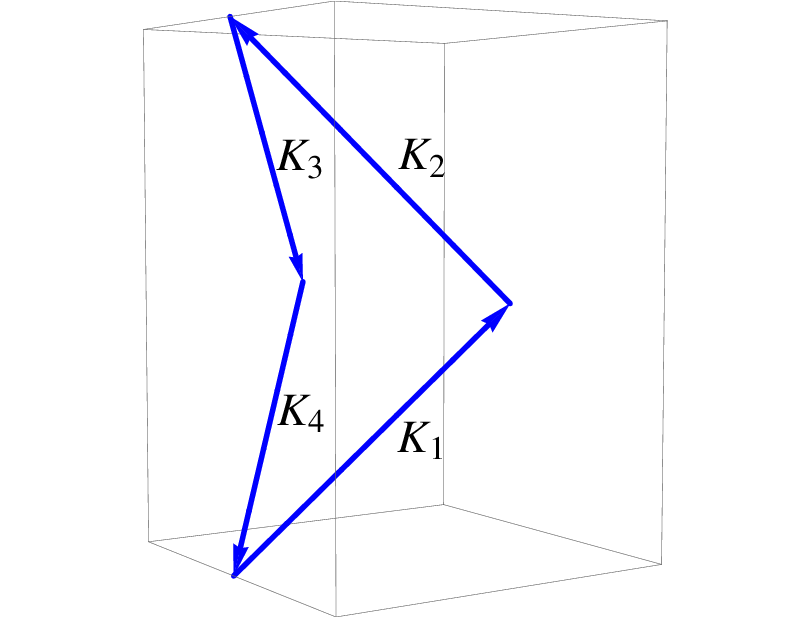
The paper is organized as follows. In section 2 we review the map to a group manifold and then classify and construct the solutions of vacuum type corresponding to space-like surfaces in AdS3×S3\mbox{AdS}_{3}\times\mbox{S}^{3}. We show that three left and three right components of Noether currents related to the isometries of SL​(2,ℝ)×SU​(2)\mbox{SL}(2,\mathbb{R})\times\mbox{SU}(2) are constants both in AdS3\mbox{AdS}_{3} and S3\mbox{S}^{3} sectors. That also justifies the name vacuum type solutions. Section 3 is devoted to a parallel treatment of the problem within Pohlmeyer reduction. In addition it contains remarks on the relation of our solutions to the complex sin(h)-Gordon type equations, which for the light-like AdS3\mbox{AdS}_{3} projection degenerate to a linear equation. Then we continue in section 4 with an elaboration of the boundary behavior of our surfaces, pointing out the qualitative differences between the various classes and give a compact listing of their characteristic properties. In section 5 we calculate the regularized area for the solution which is of potential use for a map to 4-point scattering amplitudes in ss- or tt-channel configuration. Section 6 contains a summary and some conclusions. Appendices A and B contain some technical details related to the main text.

2 Space-like strings in SL​(2,ℝ)×SU​(2)\mbox{SL}(2,\mathbb{R})\times\mbox{SU}(2)

In this section we describe the AdS3×S3\mbox{AdS}_{3}\times\mbox{S}^{3} string equations in terms of group variables and integrate these equations in the vacuum sector. We use conformal worldsheet coordinates and gauge fixing conditions, based on a holomorphic structure of space-like string surfaces.

2.1 AdS3\mbox{AdS}_{3} and S3\mbox{S}^{3} as group manifolds

The AdS3\mbox{AdS}_{3} and S3\mbox{S}^{3} spaces can be realized as the group manifolds SL​(2,ℝ)\mbox{SL}(2,\mathbb{R}) and SU​(2)\mbox{SU}(2) via

g=(Y0′+Y2Y1+Y0Y1−Y0Y0′−Y2),h=(X4+i​X3X2+i​X1−X2+i​X1X4−i​X3).g=\left(\begin{array}[]{cr}Y^{0^{\prime}}+Y^{2}&Y^{1}+Y^{0}\\ Y^{1}-Y^{0}&Y^{0^{\prime}}-Y^{2}\end{array}\right)~,~~~~~h=\left(\begin{array}[]{cr}~~X^{4}+iX^{3}&X^{2}+iX^{1}\\ -X^{2}+iX^{1}&X^{4}-iX^{3}\end{array}\right)~. (2.1)

Here YK=(Y0′,Y0,Y1,Y2)Y^{K}=(Y^{0^{\prime}},Y^{0},Y^{1},Y^{2}) are coordinates of the embedding space ℝ2,2\mathbb{R}^{2,2} and the equation for the hyperboloid

Y⋅Y≡−Y0′2−Y02+Y12+Y22=−1,Y\cdot Y\equiv-Y_{0^{\prime}}^{2}-Y_{0}^{2}+Y_{1}^{2}+Y_{2}^{2}=-1~, (2.2)

which defines the AdS3\mbox{AdS}_{3} space, is equivalent to g∈SL​(2,ℝ)g\in\mbox{SL}(2,\mathbb{R}). Similarly, the equation for S3\mbox{S}^{3} embedded in ℝ4\mathbb{R}^{4}

X⋅X≡X12+X22+X32+X42=1X\cdot X\equiv X_{1}^{2}+X_{2}^{2}+X_{3}^{2}+X_{4}^{2}=1 (2.3)

is equivalent to h∈SU​(2)h\in\mbox{SU}(2).

Let us introduce the following basis in 𝔰​𝔩​(2,ℝ)\mathfrak{sl}(2,\mathbb{R})

𝐭0=(01−10),𝐭1=(0110),𝐭2=(100−1).{\bf{t}}_{0}=\left(\begin{array}[]{cr}~0&1\\ -1&0\end{array}\right)~,~~~~{\bf{t}}_{1}=\left(\begin{array}[]{cr}0&~1\\ 1&~0\end{array}\right)~,~~~~{\bf{t}}_{2}=\left(\begin{array}[]{cr}1&~0\\ 0&-1\end{array}\right)~. (2.4)

These three matrices 𝐭μ{\bf t}_{\mu} (μ=0,1,2)(\mu=0,1,2) satisfy the relations

𝐭μ​𝐭ν=ημ​ν​𝐈+ϵμ​νρ​𝐭ρ,{\bf{t}}_{\mu}\,{\bf{t}}_{\nu}=\eta_{\mu\nu}\,{\bf I}+\epsilon_{\mu\nu}\,^{\rho}\,{\bf{t}}_{\rho}~, (2.5)

where ημ​ν=diag​(−1,1,1)\eta_{\mu\nu}=\mbox{diag}(-1,1,1) and ϵμ​ν​ρ\epsilon_{\mu\nu\rho} is the Levi-Civita tensor with ϵ012=1\epsilon_{012}=1. The inner product defined by ⟨𝐭μ​𝐭ν⟩≡12​tr​(𝐭μ​𝐭ν)=ημ​ν\langle\,{\bf t}_{\mu}\,{\bf t}_{\nu}\,\rangle\equiv\frac{1}{2}\,\mbox{tr}({\bf t}_{\mu}\,{\bf t}_{\nu})=\eta_{\mu\nu} provides the isometry between 𝔰​𝔩​(2,ℝ)\mathfrak{sl}(2,\mathbb{R}) and 3d Minkowski space.

As a basis in 𝔰​𝔲​(2)\mathfrak{su}(2) we use the anti-hermitian matrices 𝐬n=i​𝝈n{\bf s}_{n}=i\boldsymbol{\sigma}_{n} (n=1,2,3)(n=1,2,3), where 𝝈n\boldsymbol{\sigma}_{n} are the Pauli matrices (𝝈1=𝐭1,\boldsymbol{\sigma}_{1}={\bf t}_{1}, 𝝈2=−i​𝐭0\,\boldsymbol{\sigma}_{2}=-i{\bf t}_{0}, 𝝈3=𝐭2\,\boldsymbol{\sigma}_{3}={\bf t}_{2}). Here one has the algebra

𝐬m​𝐬n=−δm​n​𝐈−ϵm​n​l​𝐬l,{\bf s}_{m}\,{\bf s}_{n}=-\delta_{mn}\,{\bf I}-\epsilon_{mnl}\,{\bf s}_{l}~, (2.6)

and the inner product is introduced by a similarly normalized trace, but with the negative sign ⟨𝐬m​𝐬n⟩≡−12​tr​(𝐬m​𝐬n)=δm​n\langle{\bf s}_{m}\,{\bf s}_{n}\rangle\equiv-\frac{1}{2}\,\mbox{tr}({\bf s}_{m}\,{\bf s}_{n})=\delta_{mn}. That provides the isometry with ℝ3\mathbb{R}^{3}.

Using (2.4), eq. (2.1) can be written as g=Y0′​𝐈+Yμ​𝐭μ,g=Y^{0^{\prime}}\,{\bf I}+Y^{\mu}\,{\bf t}_{\mu}, h=X4​𝐈+Xn​𝐬n~h=X_{4}\,{\bf I}+X_{n}\,{\bf s}_{n}. The inverse group elements respectively become g−1=Y0′​𝐈−Yμ​𝐭μ,g^{-1}=Y^{0^{\prime}}\,{\bf I}-Y^{\mu}\,{\bf t}_{\mu},~ h−1=X4​𝐈−Xn​𝐬nh^{-1}=X_{4}\,{\bf I}-X_{n}\,{\bf s}_{n}. With the help of (2.5) and (2.6) one then finds the correspondence between the metric tensors

⟨(g−1​d​g)​(g−1​d​g)⟩=d​Y⋅d​Y,⟨(h−1​d​h)​(h−1​d​h)⟩=d​X⋅d​X.\langle\,(g^{-1}\,dg)\,(g^{-1}\,dg)\rangle=dY\cdot dY~,~~~~~~\langle\,(h^{-1}\,dh)\,(h^{-1}\,dh)\rangle=dX\cdot dX~. (2.7)

We use these relations in the next subsection to write the string equations in terms of the group variables.

2.2 String description in terms of group variables

We consider space-like surfaces in AdS3×S3\mbox{AdS}_{3}\times\mbox{S}^{3}. They can be parameterized by conformal complex worldsheet coordinates z=12​(σ+i​τ),z¯=12​(σ−i​τ)z=\frac{1}{2}(\sigma+i\tau),~\bar{z}=\frac{1}{2}(\sigma-i\tau). In terms of group variables we then get a pair of fields g⁡(z,z¯)g(z,\bar{z}) and h⁡(z,z¯)h(z,\bar{z}), with g∈SL​(2,ℝ)g\in\mbox{SL}(2,\mathbb{R}) and h∈SU​(2)h\in\mbox{SU}(2). Using the notation ∂≡∂σ−i∂τ\partial\equiv\partial_{\sigma}-i\partial_{\tau}, ∂¯≡∂σ+i∂τ\,\bar{\partial}\equiv\partial_{\sigma}+i\partial_{\tau}, the conformal gauge conditions can be written as

⟨(g−1​∂g)2⟩+⟨(h−1​∂h)2⟩=0=⟨(g−1​∂¯​g)2⟩+⟨(h−1​∂¯​h)2⟩.\langle\,\left(g^{-1}\,\partial g\right)^{2}\,\rangle+\langle\,\left(h^{-1}\,\partial h\,\right)^{2}\,\rangle=0=\langle\left(g^{-1}\,\bar{\partial}g\,\right)^{2}\,\rangle+\langle\,\left(h^{-1}\,\bar{\partial}h\right)^{2}\,\rangle~. (2.8)

The string action in this gauge corresponds to the sigma model on SL​(2,ℝ)×SU​(2)\mbox{SL}(2,\mathbb{R})\times\mbox{SU}(2)

S=λ4​π​∫d​σ​d​τ​[⟨(g−1​∂g)​(g−1​∂¯​g)⟩+⟨(h−1​∂h)​(h−1​∂¯​h)⟩],S=\frac{\sqrt{\lambda}}{4\pi}\int\mbox{d}\sigma\mbox{d}\tau~[\langle\,(g^{-1}\,\partial g)\,(g^{-1}\,\bar{\partial}g)\rangle+\langle\,(h^{-1}\,\partial h)\,\,(h^{-1}\,\bar{\partial}h)\rangle]~, (2.9)

where λ\lambda is a coupling constant. The variation of (2.9) leads to the equations of motion

∂(g−1​∂¯​g)+∂¯​(g−1​∂g)=0,∂(h−1​∂¯​h)+∂¯​(h−1​∂h)=0.\partial\left(g^{-1}\,\bar{\partial}g\right)+\bar{\partial}\left(g^{-1}\,\partial g\right)=0~,\quad\quad\quad\partial\left(h^{-1}\,\bar{\partial}h\right)+\bar{\partial}\left(h^{-1}\,\partial h\right)=0~. (2.10)

From these equations follow the holomorphicity conditions

∂¯​⟨(g−1​∂g)2⟩=0=∂⟨(g−1​∂¯​g)2⟩,∂¯​⟨(h−1​∂h)2⟩=0=∂⟨(h−1​∂¯​h)2⟩,\bar{\partial}\langle\,\left(g^{-1}\,\partial g\right)^{2}\,\rangle=0=\partial\langle\left(g^{-1}\,\bar{\partial}g\right)^{2}\,\rangle~,\quad\bar{\partial}\langle\,\left(h^{-1}\,\partial h\right)^{2}\rangle=0=\partial\langle\left(h^{-1}\,\bar{\partial}h\right)^{2}\,\rangle~, (2.11)

for the diagonal components of the induced metric tensors on SL​(2,ℝ)\mbox{SL}(2,\mathbb{R}) and on SU​(2)\mbox{SU}(2) separately. These conditions, together with (2.8), allow to use the gauge

⟨(g−1​∂g)2⟩=−1=⟨(g−1​∂¯​g)2⟩,⟨(h−1​∂h)2⟩=1=⟨(h−1​∂¯​h)2⟩.\langle\,\left(g^{-1}\,\partial g\right)^{2}\,\rangle=-1=\langle\,\left(g^{-1}\,\bar{\partial}g\right)^{2}\rangle~,\quad\quad\langle\left(h^{-1}\,\partial h\right)^{2}\,\rangle=1=\langle\left(h^{-1}\,\bar{\partial}h\right)^{2}\,\rangle~. (2.12)

The remaining freedom of conformal transformations z↦f⁡(z)z\mapsto f(z) in this gauge is given by translations z↦z+z0z\mapsto z+z_{0} and the reflection z↦−zz\mapsto-z. One can also consider z↦−z¯z\mapsto-\bar{z}, which corresponds to the reflection σ↦−σ\sigma\mapsto-\sigma.

In the real worldsheet coordinates (σ,τ)(\sigma,\tau) the equations of motion (2.10) read

∂σ(g−1​∂σg)+∂τ(g−1​∂τg)=0,∂σ(h−1​∂σh)+∂τ(h−1​∂τh)=0,\partial_{\sigma}\left(g^{-1}\,\partial_{\sigma}g\right)+\partial_{\tau}\left(g^{-1}\,\partial_{\tau}g\right)=0~,\quad\quad\quad\partial_{\sigma}\left(h^{-1}\,\partial_{\sigma}h\right)+\partial_{\tau}\left(h^{-1}\,\partial_{\tau}h\right)=0~, (2.13)

and the gauge fixing conditions (2.12) are equivalent to

⟨(g−1​∂τg)2⟩−⟨(g−1​∂σg)2⟩=\displaystyle\langle\,\left(g^{-1}\,\partial_{\tau}g\right)^{2}\,\rangle-\langle\,\left(g^{-1}\,\partial_{\sigma}g\right)^{2}\,\rangle= 1,\displaystyle 1~, ⟨(h−1​∂σh)2⟩−⟨(h−1​∂τh)2⟩=\displaystyle\quad\langle\,\left(h^{-1}\,\partial_{\sigma}h\right)^{2}\,\rangle-\langle\,\left(h^{-1}\,\partial_{\tau}h\right)^{2}\,\rangle= 1,\displaystyle 1~, (2.14)
⟨(g−1​∂σg)​(g−1​∂τg)⟩=\displaystyle\langle\,\left(g^{-1}\,\partial_{\sigma}g\right)\,\left(g^{-1}\,\partial_{\tau}g\right)\,\rangle= 0,\displaystyle 0~, ⟨(h−1​∂σh)​(h−1​∂τh)⟩=\displaystyle\quad\langle\,\left(h^{-1}\,\partial_{\sigma}h\right)\,\left(h^{-1}\,\partial_{\tau}h\right)\,\rangle= 0.\displaystyle 0~.

The isometry transformations of the group manifolds are given by the left-right multiplications

g↦gLggR,h↦hLhhR,g\mapsto g_{{}_{L}}\,g\,g_{{}_{R}}~,\quad\quad h\mapsto h_{{}_{L}}\,h\,h_{{}_{R}}~, (2.15)

with constant matrices gL,g_{{}_{L}}, gRg_{{}_{R}} ∈SL​(2,ℝ)\in\mbox{SL}(2,\mathbb{R}) and hL,h_{{}_{L}}, hRh_{{}_{R}} ∈SU​(2).\in\mbox{SU}(2). They leave the equations of motion (2.13) and the gauge fixing conditions (2.14) invariant. The system (2.13)-(2.14) is also invariant under the discrete transformations g↦g−1g\mapsto g^{-1} and h↦h−1h\mapsto h^{-1}, which correspond to the reflections of Y0Y^{0}, Y1Y^{1}, Y2Y^{2} and X1X^{1}, X2,X^{2}, X3X^{3}, respectively. Hence, the composition of h↦hLhhRh\mapsto h_{{}_{L}}\,h\,h_{{}_{R}} and h↦h−1h\mapsto h^{-1} form the complete group of isometry transformations of SU​(2).\mbox{SU}(2). The complete isometry group of SL​(2,ℝ)\mbox{SL}(2,\mathbb{R}) is obtained as a composition of g↦gLggRg\mapsto g_{{}_{L}}\,g\,g_{{}_{R}}, g↦g−1g\mapsto g^{-1} and g↦𝐭1​g​𝐭1g\mapsto{\bf t}_{1}\,g\,{\bf t}_{1}, where the latter corresponds to the reflection of Y0Y^{0} and Y2Y^{2}.

Using the covariant notation: (σ,τ)=(ξ1,ξ2)(\sigma,\tau)=(\xi^{1},\xi^{2}), ∂a=∂ξa\partial_{a}=\partial_{\xi^{a}} (a=1,2)(a=1,2), the induced metric tensors on the SL​(2,ℝ)\mbox{SL}(2,\mathbb{R}) and SU​(2)\mbox{SU}(2) projections can be written as22 2 In this paper (as in [6]) the index ss is used for some variables of the spherical part to distinguish them from similar variables of the AdS part.

fa​b=⟨(g−1​∂ag)​(g−1​∂bg)⟩,(fs)a​b=⟨(h−1​∂ah)​(h−1​∂bh)⟩.f_{ab}=\langle\,\left(g^{-1}\,\partial_{a}g\right)\left(g^{-1}\,\partial_{b}g\right)\,\rangle~,\quad(f_{s})_{ab}=\langle\,\left(h^{-1}\,\partial_{a}h\right)\left(h^{-1}\,\partial_{b}h\right)\,\rangle~. (2.16)

In the next two subsections we construct solutions corresponding to constant fa​bf_{ab} and (fs)a​b(f_{s})_{ab}. First we consider the SU​(2)\mbox{SU}(2) projection, since it is easier to treat. The same method then we apply to the SL​(2,ℝ)\mbox{SL}(2,\mathbb{R}) part.

2.3 Vacuum solutions in SU​(2)\mbox{SU}(2)

Let us introduce 𝔰​𝔲​(2)\mathfrak{su}(2) valued fields related to the right derivatives of hh

Rσ=h−1​∂σh,Rτ=h−1​∂τh.R_{\sigma}=h^{-1}\,\partial_{\sigma}h~,\quad\quad\quad R_{\tau}=h^{-1}\,\partial_{\tau}h~. (2.17)

These fields obey the zero curvature condition

∂τRσ−∂σRτ=[Rσ,Rτ],\partial_{\tau}R_{\sigma}-\partial_{\sigma}R_{\tau}=[R_{\sigma},\,R_{\tau}]~, (2.18)

and the second equation in (2.13) is equivalent to

∂σRσ+∂τRτ=0.\partial_{\sigma}R_{\sigma}+\partial_{\tau}R_{\tau}=0~. (2.19)

The norms and the scalar product of RσR_{\sigma} and RτR_{\tau} define the induced metric tensor on the SU​(2)\mbox{SU}(2) projection. We denote the norm of RτR_{\tau} by ρs\rho_{s}, and write the SU​(2)\mbox{SU}(2) part of the gauge fixing conditions (2.14) in the form

⟨Rσ​Rσ⟩=1+ρs2,⟨Rτ​Rτ⟩=ρs2,⟨Rσ​Rτ⟩=0.\langle\,R_{\sigma}\,R_{\sigma}\,\rangle=1+\rho_{s}^{2}~,\quad\quad\langle\,R_{\tau}\,R_{\tau}\,\rangle=\rho_{s}^{2}~,\quad\quad\langle\,R_{\sigma}\,R_{\tau}\,\rangle=0~. (2.20)

Our aim is to describe solutions of (2.17)-(2.20) for constant ρs\rho_{s}. The vectors RσR_{\sigma}, Rτ\,R_{\tau} and [Rσ,Rτ][R_{\sigma},R_{\tau}] form an orthogonal basis in 𝔰​𝔲​(2)\mathfrak{su}(2). Expanding the first derivatives of RσR_{\sigma} and RτR_{\tau} in this basis, from (2.18)-(2.20) one finds that they have vanishing projections on RσR_{\sigma} and Rτ\,R_{\tau}. Therefore, the first derivatives can be written as33 3 The coefficients on the r.h.s are interpreted as the matrix elements of the second fundamental form.

∂σRσ\displaystyle\partial_{\sigma}R_{\sigma} =a⁡[Rσ,Rτ],\displaystyle=a\,[R_{\sigma},R_{\tau}]~, ∂τRσ\displaystyle\partial_{\tau}R_{\sigma} =b⁡[Rσ,Rτ],\displaystyle=b\,[R_{\sigma},R_{\tau}]~, (2.21)
∂σRτ\displaystyle\partial_{\sigma}R_{\tau} =(b−1)​[Rσ,Rτ],\displaystyle=(b-1)\,[R_{\sigma},R_{\tau}]~, ∂τRτ\displaystyle\partial_{\tau}R_{\tau} =−a⁡[Rσ,Rτ].\displaystyle=-a\,[R_{\sigma},R_{\tau}]~.

The consistency conditions of this system are given by the equations

∂σb=∂τa,∂τb=−∂σa,a2+b2−b=0.\partial_{\sigma}b=\partial_{\tau}a~,\quad\quad\partial_{\tau}b=-\partial_{\sigma}a~,\quad\quad a^{2}+b^{2}-b=0~. (2.22)

From the first two equations follows that the coefficients aa and bb are harmonic functions a=f1​(z)+f¯1​(z¯)a=f_{1}(z)+\bar{f}_{1}(\bar{z}), b=f2​(z)+f¯2​(z¯)\,\,b=f_{2}(z)+\bar{f}_{2}(\bar{z}), with f2′​(z)=i​f1′​(z)f_{2}^{\prime}(z)=if_{1}^{\prime}(z). Then, the third equation of (2.22) leads to f1′​(z)=0f_{1}^{\prime}(z)=0, which means that aa and bb are (σ,τ)(\sigma,\tau)-independent. Due to the algebraic relation (2.22), the coefficients aa and bb are parameterized by one angle variable

a=sinϕscosϕs,b=cos2ϕs,ϕs∈[0,π).a=\sin\phi_{s}\,\cos\phi_{s}~,\quad\quad b=\cos^{2}\phi_{s}~,\quad\quad\phi_{s}\in[0,\pi)~. (2.23)

As a result, the following linear combination

R0=sin⁡ϕs​Rσ+cos⁡ϕs​RτR_{0}=\sin\phi_{s}\,R_{\sigma}+\cos\phi_{s}\,R_{\tau} (2.24)

is constant.

Now we introduce 𝔰​𝔲​(2)\mathfrak{su}(2) valued fields with the left derivatives

Lσ=∂σh​h−1,Lτ=∂τh​h−1,L_{\sigma}=\partial_{\sigma}h\,h^{-1}~,\quad\quad L_{\tau}=\partial_{\tau}h\,h^{-1}~, (2.25)

which are related to the right fields in a standard way

Lσ=h​Rσ​h−1,Lτ=h​Rτ​h−1.L_{\sigma}=hR_{\sigma}h^{-1}~,\quad\quad L_{\tau}=hR_{\tau}h^{-1}~. (2.26)

The differentiations of (2.26) lead to a system similar to (2.21)

∂σLσ=\displaystyle\partial_{\sigma}L_{\sigma}= a⁡[Lσ,Lτ],\displaystyle a\,[L_{\sigma},L_{\tau}]~, ∂τLσ\displaystyle\partial_{\tau}L_{\sigma} =(b−1)​[Lσ,Lτ],\displaystyle=(b-1)\,[L_{\sigma},L_{\tau}]~, (2.27)
∂σLτ=\displaystyle\partial_{\sigma}L_{\tau}= b⁡[Lσ,Lτ],\displaystyle b\,[L_{\sigma},L_{\tau}]~, ∂τLτ\displaystyle\partial_{\tau}L_{\tau} =−a⁡[Lσ,Lτ],\displaystyle=-a\,[L_{\sigma},L_{\tau}]~,

and one finds that the linear combination

L0=cos⁡ϕs​Lσ−sin⁡ϕs​LτL_{0}=\cos\phi_{s}\,L_{\sigma}-\sin\phi_{s}\,L_{\tau} (2.28)

is also (σ,τ)(\sigma,\tau)-independent.

From (2.24) and (2.28) follows that the field hh satisfies the equations

∂h∂ls=L0​h,∂h∂rs=h​R0,\frac{\partial h}{\partial l_{s}}=L_{0}\,h~,\quad\quad\quad\quad\frac{\partial h}{\partial r_{s}}=h\,R_{0}~, (2.29)

where the new coordinates (ls,rs)(l_{s},r_{s}) are related to (σ,τ)(\sigma,\tau) by the rotation

ls=cosϕsσ−sinϕsτ,rs=sinϕsσ+cosϕsτ.l_{s}=\cos\phi_{s}\,\,\sigma-\sin\phi_{s}\,\,\tau~,\quad r_{s}=\sin\phi_{s}\,\,\sigma+\cos\phi_{s}\,\,\tau~. (2.30)

The integration of the system (2.29) is straightforward and yields

h=els​L0​h0​ers​R0,h=e^{l_{s}\,L_{0}}\,h_{0}\,e^{r_{s}\,R_{0}}~, (2.31)

with an integration constant h0∈SU​(2)h_{0}\in\mbox{SU}(2). The isometry transformation h↦h​h0−1h\mapsto h\,h_{0}^{-1} brings the solution to the form h=els​L0​ers​R1,h=e^{l_{s}\,L_{0}}\,e^{r_{s}\,R_{1}},\, with R1=h0​Rs​h0−1R_{1}=h_{0}\,R_{s}\,h_{0}^{-1}. Denoting L0L_{0} by LsL_{s} and R1R_{1} by RsR_{s}, we obtain

h=els​Ls​ers​Rs.h=e^{l_{s}\,L_{s}}\,e^{r_{s}\,R_{s}}~. (2.32)

This field indeed solves equation (2.19) for any pair of constant vectors LsL_{s} and RsR_{s}.

To verify the orthonormality conditions (2.20) we calculate the induced metric tensor in the coordinates (ls,rs)\,(l_{s},r_{s})\,. From (2.32) follows its matrix form

(fs)a​b​(ls,rs)=(⟨Ls​Ls⟩⟨Ls​Rs⟩⟨Ls​Rs⟩⟨Rs​Rs⟩).(f_{s})_{ab}(l_{s},r_{s})=\left(\begin{array}[]{cr}\langle\,L_{s}\,L_{s}\,\rangle&\langle L_{s}\,R_{s}\,\rangle\\[5.69046pt] \langle\,L_{s}\,R_{s}\,\rangle&\langle R_{s}\,R_{s}\,\rangle\end{array}\right)~. (2.33)

On the other hand, the map (2.30) defines the same tensor as

M⁡(1+ρs200ρs2)​MT=(ρs2+cos2⁡ϕssinϕscosϕssinϕscosϕsρs2+sin2⁡ϕs),M\,\left(\begin{array}[]{cr}1+\rho_{s}^{2}&0\\[2.84544pt] 0&\rho_{s}^{2}\end{array}\right)\,M^{T}=\left(\begin{array}[]{cr}\rho_{s}^{2}+\cos^{2}\phi_{s}&\sin\phi_{s}\cos\phi_{s}\\[5.69046pt] \sin\phi_{s}\cos\phi_{s}&\rho_{s}^{2}+\sin^{2}\phi_{s}\end{array}\right)~, (2.34)

where MM is the rotation matrix in (2.30). Comparing (2.33) and (2.34), one finds

⟨LsLs⟩=ρs2+cos2ϕs,⟨RsRs⟩=ρs2+sin2ϕs,⟨LsRs⟩=sinϕscosϕs.\langle\,L_{s}\,L_{s}\,\rangle=\rho_{s}^{2}+\cos^{2}\phi_{s}~,\quad\langle\,R_{s}\,R_{s}\,\rangle=\rho_{s}^{2}+\sin^{2}\phi_{s}~,\quad\langle\,L_{s}\,R_{s}\,\rangle=\sin\phi_{s}\,\cos\phi_{s}~. (2.35)

The obtained norms of LsL_{s} and RsR_{s} are consistent with (2.28) and (2.24). A new result from this calculation is the scalar product ⟨Ls​Rs⟩\langle\,L_{s}\,R_{s}\,\rangle, which defines the angle between these vectors.

Refer to caption Refer to caption
(a) (b)
Figure 1: The pair (Ls,Rs)(L_{s},\,R_{s}) in the first plot is identified with two vectors in ℝ3\mathbb{R}^{3} located in the plane (3,1)(3,1). Similarly, LL and RR in the second plot are 3d Minkowski vectors with vanishing time components.

Now we describe how to factorize the left-right symmetry (2.15) and parameterize the SUL​(2)⊗SUR​(2)\mbox{SU}_{L}(2)\otimes\mbox{SU}_{R}(2) orbits of solutions by the pairs (ρs,ϕs)(\rho_{s},\phi_{s}).

Since the general case (2.31) reduces to (2.32) by right (or left) multiplications, it is enough to classify the fields (2.32). This factorized form of solutions is invariant under the similarity transformations h↦hLhhL−1h\mapsto h_{{}_{L}}\,h\,h_{{}_{L}}^{-1}, which rotate the vectors LsL_{s} and RsR_{s} by the adjoint representation: Ls↦hLLshL−1,L_{s}\mapsto h_{{}_{L}}\,L_{s}\,h_{{}_{L}}^{-1}, Rs↦hLRshL−1\,R_{s}\mapsto h_{{}_{L}}\,R_{s}\,h_{{}_{L}}^{-1}. The adjoint representation is equivalent to SO​(3)\mbox{SO}(3) and it is convenient to interpret LsL_{s} and RsR_{s} as vectors in ℝ3\mathbb{R}^{3}. Using this picture, one can easily bring any pair (Ls,Rs)(L_{s},\,R_{s}) to some canonical form defined only by the scalar invariants (2.35). Note that the commutator [Ls,Rs][L_{s},\,R_{s}] transforms also by the adjoint representation, its norm is given by ⟨[Ls,Rs]2⟩=4​ρs2​(1+ρs2)\left\langle[L_{s},\,R_{s}]^{2}\right\rangle=4\rho_{s}^{2}(1+\rho_{s}^{2}) and one can use this vector to specify a canonical pair (Ls,Rs)(L_{s},\,R_{s}). We choose the pair

Ls=−ρssinϕs𝐬3+1+ρs2cosϕs𝐬1,Rs=ρscosϕs𝐬3+1+ρs2sinϕs𝐬1.L_{s}=-\rho_{s}\,\sin\phi_{s}\,{\bf s}_{3}+\sqrt{1+\rho_{s}^{2}}\,\cos\phi_{s}\,{\bf s}_{1}~,\quad\quad R_{s}=\rho_{s}\,\cos\phi_{s}\,{\bf s}_{3}+\sqrt{1+\rho_{s}^{2}}\,\sin\phi_{s}\,{\bf s}_{1}~. (2.36)

It corresponds to

[Ls,Rs]=2​ρs​1+ρs2​𝐬2,[L_{s},\,R_{s}]=2\rho_{s}\,\sqrt{1+\rho_{s}^{2}}\,{\bf s}_{2}~, (2.37)

and, in addition, the vectors LsL_{s} and RsR_{s} are oriented in some symmetric way in the (𝐬3,𝐬1)({\bf s}_{3},\,{\bf s}_{1}) plane. Namely, the two rectangles formed by the components of the vectors LsL_{s} and RsR_{s} have the same area (see fig. 1(a)). The choice (2.36) is motivated by its relevance for the generalization to the SL​(2,ℝ)\mbox{SL}(2,\mathbb{R}) case. It is also helpful to establish contact with Pohlmeyer reduction.

The calculation of the exponents els​Lse^{l_{s}L_{s}} and ers​Rse^{r_{s}R_{s}} corresponding to (2.36) is straightforward. However, in general, the solution (2.32) has a rather complicated matrix form. One can simplify it by an isometry transformation. For this purpose we rewrite (2.36) as

Ls=|Ls|​e−i​β​𝝈2​𝐬3​ei​β​𝝈2,Rs=|Rs|​e−i​γ​𝝈2​𝐬3​eγ​𝝈2,L_{s}=|L_{s}|\,e^{-i\beta\,\boldsymbol{\sigma}_{2}}\,{\bf s}_{3}\,e^{i\beta\,\boldsymbol{\sigma}_{2}}~,\quad\quad R_{s}=|R_{s}|\,e^{-i\gamma\,\boldsymbol{\sigma}_{2}}\,{\bf s}_{3}\,e^{\gamma\,\boldsymbol{\sigma}_{2}}~, (2.38)

where (|Ls|, 2​β)(|L_{s}|,\,2\beta) and (|Rs|, 2​γ)(|R_{s}|,\,2\gamma) are the polar coordinates in the (𝐬3,𝐬1)({\bf s}_{3},\,{\bf s}_{1}) plane for the vectors LsL_{s} and RsR_{s}, respectively (see fig. 1(a)). Using then (A.4) and multiplying the solution (2.32) by ei​β​𝝈2e^{i\beta\,\boldsymbol{\sigma}_{2}} from the l.h.s and by e−i​γ​𝝈2e^{-i\gamma\,\boldsymbol{\sigma}_{2}} from the r.h.s., we obtain the new solution

h=ei​l~s​𝝈3​ei​θs​𝝈2​ei​r~s​𝝈3=(cos⁡θs​ei​ξssin⁡θs​ei​ηs−sin⁡θs​e−i​ηscos⁡θs​e−i​ξs).h=e^{i\tilde{l}_{s}\,\boldsymbol{\sigma}_{3}}\,e^{i\theta_{s}\,\boldsymbol{\sigma}_{2}}\,e^{i\tilde{r}_{s}\,\boldsymbol{\sigma}_{3}}=\left(\begin{array}[]{cr}\cos\theta_{s}\,e^{i\xi_{s}}&\sin\theta_{s}\,e^{i\eta_{s}}\\[5.69046pt] -\sin\theta_{s}\,e^{-i\eta_{s}}&~\cos\theta_{s}\,e^{-i\xi_{s}}\end{array}\right)~. (2.39)

Here l~s\tilde{l}_{s} and r~s\tilde{r}_{s} are the rescaled worldsheet coordinates

l~s=|Ls|​ls,r~s=|Rs|​rs,\tilde{l}_{s}=|L_{s}|\,\,l_{s}~,\quad\quad\tilde{r}_{s}=|R_{s}|\,r_{s}~, (2.40)

ξs=l~s+r~s,\xi_{s}=\tilde{l}_{s}+\tilde{r}_{s}, ηs=l~s−r~s\eta_{s}=\tilde{l}_{s}-\tilde{r}_{s} and 2​θs=2​β−2​γ2\theta_{s}=2\beta-2\gamma corresponds to the angle between LsL_{s} and RsR_{s}

cos⁡2​θs=⟨Ls​Rs⟩|Ls|​|Rs|,2​θs∈(0,π).\cos 2\theta_{s}=\frac{\left\langle L_{s}\,R_{s}\right\rangle}{|L_{s}|\,|R_{s}|}~,\qquad\qquad\qquad 2\theta_{s}\in(0,\pi)~. (2.41)

By (2.35) one has

cot⁡2​θs=sinϕscosϕsρs​1+ρs2.\cot 2\theta_{s}=\frac{\sin\phi_{s}\,\cos\phi_{s}}{\rho_{s}\sqrt{1+\rho_{s}^{2}}}~. (2.42)

The embedding coordinates for the solution (2.39) are given by

X1=sinθssinηs,X2=sinθscosηs,X3=cosθssinξs,X4=cosθscosξs.\displaystyle X_{1}=\sin\theta_{s}\,\sin\eta_{s}~,\quad X_{2}=\sin\theta_{s}\,\cos\eta_{s}~,\quad X_{3}=\cos\theta_{s}\,\sin\xi_{s}~,\quad X_{4}=\cos\theta_{s}\,\cos\xi_{s}~. (2.43)

The pairs (X1X_{1}, X2X_{2}) and (X3X_{3}, X4X_{4}) here are on the circles

X12+X22=sin2⁡θs,X32+X42=cos2⁡θs.X_{1}^{2}+X_{2}^{2}=\sin^{2}\theta_{s}~,\quad\quad X_{3}^{2}+X_{4}^{2}=\cos^{2}\theta_{s}~. (2.44)

Therefore, eq. (2.43) describes a torus in S3⊂ℝ4S^{3}\subset\mathbb{R}^{4} with the radii sin⁡θs\sin\theta_{s} and cos⁡θs\cos\theta_{s}.

The solution (2.43) was obtained in [6] via Pohlmeyer reduction. It was shown that the mean curvature of the embedding in S3\mbox{S}^{3} is equal to

Hs=cot⁡2​θs.H_{s}=\cot 2\theta_{s}~. (2.45)

From (2.32) follows the equation

⟨Ls​h​Rs​h−1⟩=⟨Ls​Rs⟩,\langle\,L_{s}\,h\,R_{s}\,h^{-1}\,\rangle=\langle\,L_{s}\,R_{s}\,\rangle~, (2.46)

which defines a surface in SU​(2)\mbox{SU}(2) in a form independent of worldsheet coordinates. Since hh and h−1h^{-1} are linear functions of the embedding coordinates, the l.h.s. of (2.46) provides a quadric in these variables. The corresponding surface expressed in ℝ4\mathbb{R}^{4} embedding coordinates is given as an intersection of the S3⊂ℝ4S^{3}\subset\mathbb{R}^{4} and

X42​⟨Ls​Rs⟩+X4​Xn​⟨Ls​[sn,Rs]⟩−Xn​Xm​⟨Ls​sm​Rs​sn⟩=⟨Ls​Rs⟩.X_{4}^{2}\langle L_{s}R_{s}\rangle+X_{4}X_{n}\langle L_{s}[s_{n},R_{s}]\rangle-X_{n}X_{m}\langle L_{s}s_{m}R_{s}s_{n}\rangle~=~\langle L_{s}R_{s}\rangle~. (2.47)

Taking LsL_{s} and RsR_{s} from (2.38), after simple transformations one can rewrite (2.46) in the form

⟨𝐬3​h​𝐬3​h−1⟩=cos⁡2​θs,\langle\,{\bf s}_{3}\,h\,{\bf s}_{3}\,h^{-1}\,\rangle=\cos 2\theta_{s}~, (2.48)

which reproduces (2.44). Though this surface in SU(2) is described only by θs\theta_{s}, this parameter is not a complete characteristic of the SU(2) part for our system in SL​(2,ℝ)×SU(2)\mbox{SL}(2,\mathbb{R})\times\mbox{SU(2)}. Since we are in a fixed gauge, ρs\rho_{s} also has a certain gauge invariant meaning. Namely, ρs​1+ρs2​d​σ​d​τ\rho_{s}\sqrt{1+\rho_{s}^{2}}\,d\sigma\,d\tau defines the area measure on the surface induced from S3\mbox{S}^{3}.

Finally, note that LsL_{s} and RsR_{s} are related to the Noether integrals of the isometry group and therefore they have also a gauge invariant meaning.

2.4 Vacuum solutions in SL​(2,ℝ)\mbox{SL}(2,\mathbb{R})

Based on the isometry between the 𝔰​𝔩​(2,ℝ)\mathfrak{sl}(2,\mathbb{R}) algebra and 3d Minkowski space, we call a vector 𝔞∈𝔰​𝔩​(2,ℝ)\mathfrak{a}\in\mathfrak{sl}(2,\mathbb{R}) space-like if ⟨𝔞​𝔞⟩>0\langle\mathfrak{a}\,\mathfrak{a}\rangle>0, time-like if ⟨𝔞​𝔞⟩<0\langle\mathfrak{a}\,\mathfrak{a}\rangle<0 and light-like if ⟨𝔞​𝔞⟩=0\langle\mathfrak{a}\,\mathfrak{a}\rangle=0.

Note that the vector g−1​∂τgg^{-1}\partial_{\tau}g is space-like in the gauge (2.14). Similarly to the SU​(2)\mbox{SU}(2) case, we introduce the notation ρ2≡⟨(g−1​∂τg)2⟩\rho^{2}\equiv\langle(g^{-1}\partial_{\tau}g)^{2}\rangle and write the induced metric tensor on the SL​(2,ℝ)\mbox{SL}(2,\mathbb{R}) projection in the form44 4 This form differs from the one used in [6]. There the (τ​τ)(\tau\tau)-component of the induced metric tensor was denoted by 1+ρ21+\rho^{2} for the space-like surfaces and by 1−ρ21-\rho^{2} for the time-like ones. Note also, that in our convention σ\sigma is time-like in the time-like case.

fa​b​(σ,τ)=(ρ2−100ρ2).f_{ab}(\sigma,\tau)=\left(\begin{array}[]{cr}\rho^{2}-1&0\\ 0&\rho^{2}\end{array}\right)~. (2.49)

The sum with the SU​(2)\mbox{SU}(2) metric (2.20) gives the total metric induced from SL​(2,ℝ)×SU​(2)\mbox{SL}(2,\mathbb{R})\times\mbox{SU}(2) and is by construction a multiple of the identity matrix. The metric (2.49) is space-like if ρ2>1,\rho^{2}>1,\, it is time-like if 0<ρ2<10<\rho^{2}<1\, and it becomes light-like if ρ2=1\rho^{2}=1. The last case corresponds to a degenerate metric with a light-like vector g−1​∂σgg^{-1}\partial_{\sigma}g.

We consider constant ρ2\rho^{2} and apply the scheme of the previous subsection. The case of light-like RσR_{\sigma} is special and we consider it separately. If RσR_{\sigma} is space-like or time-like, the vectors Rσ,R_{\sigma}, Rτ\,R_{\tau}\, and [Rσ,Rτ]\,[R_{\sigma},\,R_{\tau}] form an orthonormal basis in 𝔰​𝔩​(2,ℝ)\mathfrak{sl}(2,\mathbb{R}). Repeating then the same steps as in SU​(2)\mbox{SU}(2) we come to the factorized type solution (2.32)

g=el​L​er​R.g=e^{l\,L}\,e^{r\,R}~. (2.50)

Here (L,R)(L,\,R) is a pair of constant elements of the 𝔰​𝔩​(2,ℝ)\mathfrak{sl}(2,\mathbb{R}) algebra and (OPENl,r)l,r) are worldsheet coordinates obtained from (σ,τ)(\sigma,\tau) by a rotation on an angle ϕ\phi which parameterizes the coefficients of the linear system (see (2.21))

a=⟨∂σRσ​[Rσ,Rτ]⟩⟨[Rσ,Rτ]2⟩,b=⟨∂τRσ​[Rσ,Rτ]⟩⟨[Rσ,Rτ]2⟩.a=\frac{\langle\,\partial_{\sigma}R_{\sigma}\,[R_{\sigma},R_{\tau}]\,\rangle}{\langle\,[R_{\sigma},R_{\tau}]^{2}\,\rangle}~,\qquad b=\frac{\langle\,\partial_{\tau}R_{\sigma}\,[R_{\sigma},R_{\tau}]\,\rangle}{\langle\,[R_{\sigma},R_{\tau}]^{2}\,\rangle}~. (2.51)

Now Rσ=g−1​∂σg,R_{\sigma}=g^{-1}\partial_{\sigma}g, Rτ=g−1​∂τgR_{\tau}=g^{-1}\partial_{\tau}g\, and a,\,a, bb satisfy again (2.22). For further convenience, we use here a different parameterization

a=−sinϕcosϕ,b=sin2ϕ,ϕ∈(−π/2,π/2],a=-\sin\phi\,\cos\phi~,\quad\quad b=\sin^{2}\phi~,\quad\quad\phi\in(-\pi/2,\,\pi/2], (2.52)

which is obtained from (2.23) by the replacements cos⁡ϕs↦sin⁡ϕ,\cos\phi_{s}\mapsto\sin\phi,\, sin⁡ϕs↦−cos⁡ϕ\,\sin\phi_{s}\mapsto-\cos\phi. This provides the following (l,r)(l,\,r) coordinates (compare with (2.30))

l=cos⁡ϕ​τ+sin⁡ϕ​σ,r=sin⁡ϕ​τ−cos⁡ϕ​σ.l=\cos\phi\,\,\tau+\sin\phi\,\,\sigma~,\quad r=\sin\phi\,\,\tau-\cos\phi\,\,\sigma~. (2.53)

If RσR_{\sigma} is light-like, one gets the commutator55 5 Note that (2.54) is equivalent to [(𝐭𝟏−𝐭𝟎),𝐭𝟐]=𝟐​(𝐭𝟏−𝐭𝟎)[(\bf{t}_{1}-\bf{t}_{0}),\,\bf{t}_{2}]=2(\bf{t}_{1}-\bf{t}_{0}).

[Rσ,Rτ]=2​Rσ.[R_{\sigma},\,R_{\tau}]=2\,R_{\sigma}~. (2.54)

Hence, in this case, Rσ,R_{\sigma}, Rτ\,R_{\tau}\, and [Rσ,Rτ]\,[R_{\sigma},\,R_{\tau}] do not form a basis in 𝔰​𝔩​(2,ℝ)\mathfrak{sl}(2,\mathbb{R}). Completing RσR_{\sigma} and RτR_{\tau} in a suitable way to a basis, one can show that in the end the third independent direction is not needed to express the derivatives of RσR_{\sigma} and RτR_{\tau}. For details see the parallel discussion of this issue in the framework of Pohlmeyer reduction in section 3.3 below. Altogether the system (2.21) is modified and replaced by the linear system

∂σRσ\displaystyle\partial_{\sigma}R_{\sigma} =2​a​Rσ,\displaystyle=2a\,R_{\sigma}~, ∂τRσ\displaystyle\partial_{\tau}R_{\sigma} =2​b​Rσ,\displaystyle=2b\,R_{\sigma}~, (2.55)
∂σRτ\displaystyle\partial_{\sigma}R_{\tau} =2​(b−1)​Rσ,\displaystyle=2(b-1)\,R_{\sigma}~, ∂τRτ\displaystyle\partial_{\tau}R_{\tau} =−2​a​Rσ.\displaystyle=-2a\,R_{\sigma}~.

The consistency conditions for this system lead to the equations

∂τa−∂σb=0,∂σa+∂τb+2​(a2+b2−b)=0,\partial_{\tau}a-\partial_{\sigma}b=0~,\quad\quad\partial_{\sigma}a+\partial_{\tau}b+2(a^{2}+b^{2}-b)=0~, (2.56)

which, in contrast to other cases, do not necessarily require constant aa and bb. In section 3.3 we describe also the general solution of the consistency conditions (2.56) and indicate how to integrate the linear system (2.55). Here we identify vacuum configurations with the solutions for constant aa and bb. In this case (2.56) reduces again to a2+b2−b=0a^{2}+b^{2}-b=0 and one can use the parameterization (2.52). Constant currents (L,R)(L,\,R) are then constructed in a same way and one again obtains solutions in the factorized form (2.50). Thus, (2.50) represents solutions in the vacuum sector for all three cases: ρ2>1,\rho^{2}>1,\, ρ2<1\rho^{2}<1 and ρ2=1\rho^{2}=1 as well.

The induced metric tensor in (l,r)(l,r)-coordinates, calculated by (2.49) and (2.53), becomes

fa​b​(l,r)=(ρ2−sin2⁡ϕsin⁡ϕ​cos⁡ϕsin⁡ϕ​cos⁡ϕρ2−cos2⁡ϕ),f_{ab}(l,r)=\left(\begin{array}[]{cr}\rho^{2}-\sin^{2}\phi&\sin\phi\cos\phi\\[2.84544pt] \sin\phi\cos\phi&\rho^{2}-\cos^{2}\phi\end{array}\right), (2.57)

and comparing it with the calculation from (2.50), one finds

⟨L​L⟩=ρ2−sin2⁡ϕ,⟨R​R⟩=ρ2−cos2⁡ϕ,⟨L​R⟩=sin⁡ϕ​cos⁡ϕ.\langle\,L\,L\,\rangle=\rho^{2}-\sin^{2}\phi~,\quad\langle\,R\,R\,\rangle=\rho^{2}-\cos^{2}\phi~,\quad\langle\,L\,R\,\rangle=\sin\phi\,\cos\phi~. (2.58)

These equations fix the norm of the commutator [L,R][L,\,R] to

⟨[L,R]2⟩=4​ρ2​(1−ρ2).\left\langle\,[L,\,R]^{2}\,\right\rangle=4\rho^{2}(1-\rho^{2})~. (2.59)

Thus, [L,R][L,\,R] is time-like for space-like surfaces (ρ2>1)(\rho^{2}>1), [L,R][L,\,R] is light-like for light-like surfaces (ρ2=1\rho^{2}=1) and [L,R][L,\,R] is space-like for time-like surfaces (ρ2<0)(\rho^{2}<0).

We use these metric characteristics of the commutator [L,R][L,R] and also the scalars (2.58) to classify the fields gg by the adjoint orbits similarly to the previous subsection. Since the adjoint representation of SL​(2,ℝ)\mbox{SL}(2,\mathbb{R}) is given by the group of proper Lorentz transformations SO↑​(1,2)\mbox{SO}_{\uparrow}(1,2), the orbits can be identified with the hyperbolas and cones in 3d Minkowski space. Choosing canonical pairs (L,R)(L,R) from the orbits, one can construct solutions by (2.50) and then simplify them as in (2.39). This procedure also simplifies the form of the quadratic relation between the ℝ2,2\mathbb{R}^{2,2} embedding coordinates, which is now given by

⟨L​g​R​g−1⟩=(Y0′)2​⟨L​R⟩+Yμ​Y0′​⟨L⁡[tμ,R]⟩−Yμ​Yν​⟨L​tμ​R​tν⟩=⟨L​R⟩.\langle\,L\,g\,R\,g^{-1}\,\rangle~=(Y^{0^{\prime}})^{2}\langle LR\rangle+Y^{\mu}Y^{0^{\prime}}\langle L[t_{\mu},R]\rangle-Y^{\mu}Y^{\nu}\langle Lt_{\mu}Rt_{\nu}\rangle~=\langle\,L\,R\,\rangle~. (2.60)

It is natural to divide the solutions in three classes according to the signature of the induced metric tensor and then continue classification inside the classes.

Before starting classification it is useful to note that the reflection freedom σ↦−σ\sigma\mapsto-\sigma allows to set a≤0a\leq 0 (see eqs. (2.51)-(2.52) and (2.55)). This corresponds to ϕ∈[0,π/2]\phi\in[0,\pi/2]. Below we assume this condition.

1. Space-like surfaces (ρ2>1)\,\,(\rho^{2}>1).

This case corresponds to space-like LL, RR and time-like [L,R][L,\,R]. One can take the commutator [L,R][L,\,R] proportional to 𝐭0{\bf t}_{0}. However, in contrast to the SU​(2)\mbox{SU}(2) case there are two possibilities

[L,R]=±2​ρ​ρ2−1​𝐭0,[L,\,R]=\pm 2\rho\sqrt{\rho^{2}-1}\,{\bf t}_{0}~, (2.61)

which are not on the same adjoint orbit. These two cases are related by the discrete isometry transformation g↦𝐭1​g​𝐭1g\mapsto{\bf t}_{1}\,g\,{\bf t}_{1}.

Let us consider the negative sign in (2.61) and choose the pair

L=ρ​cos⁡ϕ​𝐭2+ρ2−1​sin⁡ϕ​𝐭1,R=ρ​sin⁡ϕ​𝐭2−ρ2−1​cos⁡ϕ​𝐭1.L=\rho\cos\phi\,{\bf t}_{2}+\sqrt{\rho^{2}-1}\,\sin\phi\,{\bf t}_{1}~,\quad\quad R=\rho\sin\phi\,{\bf t}_{2}-\sqrt{\rho^{2}-1}\,\cos\phi\,{\bf t}_{1}~. (2.62)

Using the same trick as in (2.38), based now on (A.7), we first rewrite (2.62) in the form

L=|L|​e−β​𝐭0​𝐭2​eβ​𝐭0,R=|R|​e−γ​𝐭0​𝐭2​eγ​𝐭0,L=|L|\,e^{-\beta\,{\bf t}_{0}}\,{\bf t}_{2}\,e^{\beta\,{\bf t}_{0}}~,\quad\quad R=|R|\,e^{-\gamma\,{\bf t}_{0}}\,{\bf t}_{2}\,e^{\gamma\,{\bf t}_{0}}~, (2.63)

where |L|=ρ2−sin2⁡ϕ,|L|=\sqrt{\rho^{2}-\sin^{2}\phi}, |R|=ρ2−cos2⁡ϕ,\,|R|=\sqrt{\rho^{2}-\cos^{2}\phi}, and (2​β,2\beta,\, 2​γ2\gamma) are the polar angles in the (𝐭2,𝐭1)({\bf t}_{2},{\bf t}_{1}) plane, (see fig. 1(b)). Then, as in (2.39), the left-right multiplications reduce the solution (2.50) to

g=el~​𝐭2​eθ​𝐭0​er~​𝐭2=(cos⁡θ​eξsin⁡θ​eη−sin⁡θ​e−ηcos⁡θ​e−ξ).g=e^{\tilde{l}\,{\bf t}_{2}}\,e^{\theta\,{\bf t}_{0}}\,e^{\tilde{r}\,{\bf t}_{2}}=\left(\begin{array}[]{cr}\cos\theta\,e^{\xi}&\sin\theta\,e^{\eta}\\[2.84544pt] -\sin\theta\,e^{-\eta}&~\cos\theta\,e^{-\xi}\end{array}\right)~. (2.64)

Here l~=|L|​l\tilde{l}=|L|\,l and r~=|R|​r\tilde{r}=|R|\,r are the rescaled worldsheet coordinates, ξ=l~+r~,\,\xi=\tilde{l}+\tilde{r}, η=l~−r~\eta=\tilde{l}-\tilde{r} and 2​θ=2​β−2​γ2\theta=2\beta-2\gamma is the angle between the vectors (2.62), with

cot⁡2​θ=sin⁡ϕ​cos⁡ϕρ​ρ2−1,θ∈(0,π/4].\cot 2\theta=\frac{\sin\phi\,\cos\phi}{\rho\sqrt{\rho^{2}-1}}~,\qquad\qquad\theta\in(0,\pi/4]~. (2.65)

The embedding coordinates for the solution (2.64) are given by

Y0′=cos⁡θ​cosh⁡ξ,Y0=sin⁡θ​cosh⁡η,Y1=sin⁡θ​sinh⁡η,Y2=cos⁡θ​sinh⁡ξ.\displaystyle Y^{0^{\prime}}=\cos\theta\,\cosh\xi~,\quad Y^{0}=\sin\theta\,\cosh\eta~,\quad Y^{1}=\sin\theta\,\sinh\eta~,\quad Y^{2}=\cos\theta\,\sinh\xi~. (2.66)

This surface was also obtained in [6] by Pohlmeyer reduction. Its mean curvature is

H=cot⁡2​θ.H=\cot 2\theta~. (2.67)

Similarly to (2.48), the quadric (2.60) reduces to

(Y0)2−(Y1)2=sin2⁡θ,(Y^{0})^{2}-(Y^{1})^{2}=\sin^{2}\theta~, (2.68)

and for θ=π/4\theta=\pi/4 it reproduces the four cusp surface of [3, 1].

Like in (2.43), the shape of the surface (2.66) depends only on the parameter θ\theta, and not on ρ\rho and ϕ\phi separately. The first plot in fig. 2 shows the constant θ\theta lines on the strip with the coordinates (sin2⁡ϕ,ρ2)(\sin^{2}\phi,\,\rho^{2}). From (2.65) follows that these lines are arcs of ellipses for the space-like surfaces (ρ2>1\rho^{2}>1). One can check (see below the analog of (2.65) ) that the lines become arcs of hyperbolas for ρ2<1.\rho^{2}<1. The second plot in fig. 2 is used for a classification of the surfaces which we consider below. Note again that different points on the constant θ\theta lines describe different solutions of the system in AdS3×S3\mbox{AdS}_{3}\times\mbox{S}^{3}, though they have the same AdS3\mbox{AdS}_{3} projection.

In fig. 3 we present the surfaces in AdS3\mbox{AdS}_{3} associated with different solutions of our system. The surface (2.66) is shown in the plot 3(a).

Refer to caption Refer to caption
(a) (b)
Figure 2: The dashed lines in the first plot correspond to constant θ\theta. The left and right signs in the second plot correspond to the signs of ⟨L2⟩\langle L^{2}\rangle and ⟨R2⟩\langle R^{2}\rangle, respectively. ⟨L2⟩\langle L^{2}\rangle vanishes at the diagonal B​DBD and ⟨R2⟩\langle R^{2}\rangle at A​EAE.

2. Light-like surfaces (ρ2=1).\,\,(\rho^{2}=1).

The commutator [L,R][L,\,R] is light-like for ρ2=1\rho^{2}=1 and one has again two options

[L,R]=± 2​𝐭+≡±(𝐭0+𝐭1),[L,\,R]=\pm\,2{\bf t}_{+}\equiv\pm({\bf t}_{0}+{\bf t}_{1})~, (2.69)

which are not on the same adjoint orbit. The option [L,R]=−2​𝐭+[L,\,R]=-2{\bf t}_{+} can be realized by

L=cos⁡ϕ​𝐭2+sin⁡ϕ​𝐭+,R=sin⁡ϕ​𝐭2−cos⁡ϕ​𝐭+.L=\cos\phi\,{\bf t}_{2}+\sin\phi\,{\bf t}_{+}~,\quad\quad R=\sin\phi\,{\bf t}_{2}-\cos\phi\,{\bf t}_{+}~. (2.70)

Note that the pair (−L,−R)(-L,\,-R) has the same commutator and the scalar invariants (2.58) as (L,R)(L,R). However, these two pairs are on different adjoint orbits. We have the same situation for [L,R]=2​𝐭+[L,\,R]=2{\bf t}_{+}. Hence, for ρ2=1\rho^{2}=1, there are four sets of adjoint orbits of (L,R)(L,R) pairs. They are related to each other by discrete isometry transformations. Therefore, it is sufficient to consider only (2.70). It splits into three subcases:

2.1) ϕ=0;\phi=0;~ 2.2) ϕ=π/2;\phi=\pi/2;~ 2.3) ϕ∈(0,π/2)\phi\in(0,\pi/2).

Case 2.1. ϕ=0\phi=0\, corresponds to the point AA in fig. 2(b).

Now ⟨L​L⟩=1,\langle\,L\,L\,\rangle=1,~ ⟨R​R⟩=0,\langle\,R\,R\,\rangle=0,~ ⟨L​R⟩=0;\langle\,L\,R\,\rangle=0;~ l=τ,l=\tau,~ r=−σ.r=-\sigma. Then, eq. (2.50) yields the solution

g=eτ​𝐭2​eσ​𝐭+=(eτσ​eτ0e−τ),g=e^{\tau\,{\bf t}_{2}}\,e^{\sigma\,{\bf t}_{+}}=\left(\begin{array}[]{cr}e^{\tau}&\sigma\,e^{\tau}\\[2.84544pt] 0&e^{-\tau}\end{array}\right)~, (2.71)

with the embedding coordinates

Y0′=cosh⁡τ,Y0=σ2​eτ,Y1=σ2​eτ,Y2=sinh⁡τ.\displaystyle Y^{0^{\prime}}=\cosh\tau~,\quad Y^{0}=\frac{\sigma}{2}\,\,e^{\tau}~,\quad Y^{1}=\frac{\sigma}{2}\,\,e^{\tau}~,\quad Y^{2}=\sinh\tau~. (2.72)

The quadric (2.60) here reduces to

(Y0−Y1)​(Y0′+Y2)=0,(Y^{0}-Y^{1})(Y^{0^{\prime}}+Y^{2})=0~, (2.73)

which is realized by (2.72) in the linear form Y0−Y1=0.Y^{0}-Y^{1}=0. The surface (2.72) is given by the plot 3(b). It has two cusps at the boundary.

Case 2.2. ϕ=π/2\phi=\pi/2\, corresponds to the point BB in fig. 2(b).

Here ⟨L​L⟩=0,\langle\,L\,L\,\rangle=0,~ ⟨R​R⟩=1,\langle\,R\,R\,\rangle=1,~ ⟨L​R⟩=0;\langle\,L\,R\,\rangle=0;~ l=σl=\sigma, r=τ.~r=\tau. The solution (2.50) now becomes

g=eσ​𝐭+​eτ​𝐭2=(eτσ​e−τ0e−τ),g=e^{\sigma\,{\bf t}_{+}}\,e^{\tau\,{\bf t}_{2}}=\left(\begin{array}[]{cr}e^{\tau}&\sigma\,e^{-\tau}\\[2.84544pt] 0&e^{-\tau}\end{array}\right)~, (2.74)

with the embedding coordinates

Y0′=cosh⁡τ,Y0=σ2​e−τ,Y1=σ2​e−τ,Y2=sinh⁡τ,\displaystyle Y^{0^{\prime}}=\cosh\tau~,\quad Y^{0}=\frac{\sigma}{2}\,\,e^{-\tau}~,\quad Y^{1}=\frac{\sigma}{2}\,\,e^{-\tau}~,\quad Y^{2}=\sinh\tau~, (2.75)

and the quadric (Y0−Y1)​(Y0′−Y2)=0.(Y^{0}-Y^{1})(Y^{0^{\prime}}-Y^{2})=0. This surface is obtained from (2.73) by the reflection Y2↦−Y2Y^{2}\mapsto-Y^{2}. Hence, the plot 3(b) represents (2.75) as well.

Case 2.3. ϕ∈(0,π/2)\phi\in(0,\pi/2)\, corresponds to the segment between the points AA and BB in fig. 2(b).
In this case ⟨L​L⟩=cos2⁡ϕ>0,\langle\,L\,L\,\rangle=\cos^{2}\phi>0,\, ⟨R​R⟩=sin2⁡ϕ>0.\langle\,R\,R\,\rangle=\sin^{2}\phi>0. Here we simplify the solution (2.50) by the same trick as in (2.38)-(2.39). Using (A.8), we write (2.70) as

L=cos⁡ϕ​e−β​𝐭+​𝐭2​eβ​𝐭+,R=sin⁡ϕ​e−γ​𝐭+​𝐭2​eγ​𝐭+,L=\cos\phi\,e^{-\beta\,{\bf t}_{+}}\,{\bf t}_{2}\,e^{\beta\,{\bf t}_{+}}~,\quad\quad R=\sin\phi\,\,e^{-\gamma\,{\bf t}_{+}}\,{\bf t}_{2}\,e^{\gamma\,{\bf t}_{+}}~, (2.76)

and bring the solution (2.50) to the form el​cos⁡ϕ​𝐭2​eθ​𝐭+​er​sin⁡ϕ​𝐭2e^{l\,\cos\phi\,{\bf t}_{2}}\,e^{\theta{\bf t}_{+}}\,e^{r\,\sin\phi\,{\bf t}_{2}}, with θ=β−γ=1/sin⁡2​ϕ\theta=\beta-\gamma=1/\sin 2\phi. By the rescaling property eλ​𝐭2​𝐭+​e−λ​𝐭2=e2​λ​t+e^{\lambda{\bf t}_{2}}\,{\bf t}_{+}\,e^{-\lambda{\bf t}_{2}}=e^{2\lambda}t_{+}, we then set θ=1\theta=1 and get

g=el​cos⁡ϕ​𝐭2​e𝐭+​er​sin⁡ϕ​𝐭2=(eτeτ~0e−τ),τ~=τ​cos⁡2​ϕ+σ​sin⁡2​ϕ.g=e^{l\,\cos\phi\,{\bf t}_{2}}\,e^{{\bf t}_{+}}\,e^{r\sin\phi\,{\bf t}_{2}}=\left(\begin{array}[]{cr}e^{\tau}&e^{\tilde{\tau}}\\[2.84544pt] 0&e^{-\tau}\end{array}\right)~,\qquad\qquad\tilde{\tau}=\tau\,\cos 2\phi+\sigma\,\sin 2\phi~. (2.77)

This solution satisfies the relation ⟨𝐭2​g​𝐭2​g−1⟩=1\left\langle{\bf t}_{2}\,g\,{\bf t}_{2}\,g^{-1}\right\rangle=1, which reduces to

(Y0)2−(Y1)2=0,(Y^{0})^{2}-(Y^{1})^{2}=0~, (2.78)

and it can be treated as a limiting case of (2.68) at θ→0\theta\rightarrow 0. The embedding coordinates

Y0′=cosh⁡τ,Y0=eτ~2,Y1=eτ~2,Y2=sinh⁡τ\displaystyle Y^{0^{\prime}}=\cosh\tau~,\quad Y^{0}=\,\frac{e^{\tilde{\tau}}}{2}~,\quad Y^{1}=\frac{e^{\tilde{\tau}}}{2}~,\quad Y^{2}=\sinh\tau (2.79)

realize (2.78) by Y0−Y1=0Y^{0}-Y^{1}=0 as in (2.72). The difference with the case 2.1 is that now Y0Y^{0} and Y1Y^{1} are positive on the worldsheet. This surface is given by the plot 3(c) and has one cusp at the boundary. The line crossing the interior of AdS3\mbox{AdS}_{3} corresponds to τ¯→−∞\bar{\tau}\rightarrow-\infty. Although now the projection to AdS3\mbox{AdS}_{3} has a boundary inside AdS3\mbox{AdS}_{3}, the surface itself has there no boundary inside AdS3×S3\mbox{AdS}_{3}\times\mbox{S}^{3}, since τ¯→−∞\bar{\tau}\rightarrow-\infty is correlated with infinitely wrapping the torus in S3\mbox{S}^{3}.

Concluding this part we note that the calculation of (2.50) for LL and RR given by (2.70) leads to the answer

g=el​L​er​R=(eτμ0e−τ),μ=eτ~−cosh⁡τ−cos⁡2​ϕ​sinh⁡τsin⁡2​ϕ.g=e^{l\,L}\,e^{r\,R}=\left(\begin{array}[]{cr}e^{\tau}&\mu\\[2.84544pt] 0&e^{-\tau}\end{array}\right)~,\quad\quad\mu=\frac{e^{\tilde{\tau}}-\cosh\tau-\cos 2\phi\sinh\tau}{\sin 2\phi}~. (2.80)

The isometry transformations described above simplify its g12g_{12} component to (2.77).

The solution (2.80) provides the following embedding coordinates

Y0′=coshτ,Y0=eτ~−cosh⁡τ−cos⁡2​ϕ​sinh⁡τ2​sin⁡2​ϕ=Y1,Y2=sinhτ,\displaystyle Y^{0^{\prime}}=\cosh\tau~,\quad Y^{0}=\frac{e^{\tilde{\tau}}-\cosh\tau-\cos 2\phi\sinh\tau}{2\sin 2\phi}=Y^{1}~,\quad Y^{2}=\sinh\tau~, (2.81)

which in the limit ϕ→0\phi\rightarrow 0 and ϕ→π/2\phi\rightarrow\pi/2 reproduces (2.72) and (2.75), respectively.

3. Time-like surfaces (ρ2<1).~(\rho^{2}<1).

Here [L,R][L,\,R] is space-like and we can fix it by

[L,R]=−2​ρ​1−ρ2​𝐭1.[L,\,R]=-2\rho\sqrt{1-\rho^{2}}\,{\bf t}_{1}~. (2.82)

LL and RR are then in the plane (𝐭2,𝐭0)({\bf t}_{2},{\bf t}_{0}) and the pairs (L,R)(L,R) and (−L,−R)(-L,-R) belong to different adjoint orbits, generated by 𝐭1{\bf t}_{1}. Hence, there are two options for (L,R)(L,\,R), which are related to each other through the discrete isometry transformation g↦𝐭1​g​𝐭1g\mapsto{\bf t}_{1}\,g\,{\bf t}_{1}.

Similarly to (2.62), we choose the pair

L=ρ​cos⁡ϕ​𝐭2+1−ρ2​sin⁡ϕ​𝐭0,R=ρ​sin⁡ϕ​𝐭2−1−ρ2​cos⁡ϕ​𝐭0,L=\rho\,\cos\phi\,{\bf t}_{2}+\sqrt{1-\rho^{2}}\,\sin\phi\,{\bf t}_{0}~,\quad\quad R=\rho\,\sin\phi\,{\bf t}_{2}-\sqrt{1-\rho^{2}}\,\cos\phi\,{\bf t}_{0}~, (2.83)

which now allows all three possibilities (space-like, light-like, time-like) for both LL and RR. The corresponding nine cases are represented in fig. 2(b) inside the square ρ2<1\rho^{2}<1 and we enumerate them in the following order:

Case 3.1 ⟨L​L⟩>0\langle\,L\,L\,\rangle>0, ⟨R​R⟩>0\langle\,R\,R\,\rangle>0.

This corresponds to the area inside the triangle A​B​CABC in fig. 2(b).
Here ρ2>max​[sin2⁡ϕ,cos2⁡ϕ],\rho^{2}>\mbox{max}[\sin^{2}\phi,\,\cos^{2}\phi], which implies ρ​1−ρ2<sin⁡ϕ​cos⁡ϕ\rho\,\sqrt{1-\rho^{2}}<\sin\phi\,\cos\phi and ρ2>1/2\rho^{2}>1/2.

The space-like vectors (2.83) can be written in the form (2.38)

L=ρ2−sin2⁡ϕ​e−β​𝐭1​𝐭2​eβ​𝐭1,R=ρ2−cos2⁡ϕ​e−γ​𝐭1​𝐭2​eγ​𝐭1,L=\sqrt{\rho^{2}-\sin^{2}\phi}\,\,e^{-\beta\,{\bf t}_{1}}\,{\bf t}_{2}\,e^{\beta\,{\bf t}_{1}}~,\quad\quad R=\sqrt{\rho^{2}-\cos^{2}\phi}\,\,e^{-\gamma\,{\bf t}_{1}}\,{\bf t}_{2}\,e^{\gamma\,{\bf t}_{1}}~, (2.84)

using the boost parameters β\beta and γ\gamma. Applying then the same trick as above, we find the solution

g=el~​𝐭2​eθ​𝐭1​er~​𝐭2=(cosh⁡θ​eξsinh⁡θ​eηsinh⁡θ​e−ηcosh⁡θ​e−ξ),g=e^{\tilde{l}\,{\bf t}_{2}}\,e^{\theta\,{\bf t}_{1}}\,e^{\tilde{r}\,{\bf t}_{2}}=\left(\begin{array}[]{cr}\cosh\theta\,e^{\xi}&\sinh\theta\,e^{\eta}\\[5.69046pt] \sinh\theta\,e^{-\eta}&\cosh\theta\,e^{-\xi}\end{array}\right)~, (2.85)

where

l~=ρ2−sin2⁡ϕ​l,r~=ρ2−cos2⁡ϕ​r\tilde{l}=\sqrt{\rho^{2}-\sin^{2}\phi}\,\,l~,\quad\quad\tilde{r}=\sqrt{\rho^{2}-\cos^{2}\phi}\,\,r (2.86)

are the rescaled coordinates, ξ=l~+r~,\xi=\tilde{l}+\tilde{r}, η=l~−r~\eta=\tilde{l}-\tilde{r}, and the new boost parameter θ=β−γ>0\theta=\beta-\gamma>0 is given by

tanh⁡2​θ=ρ​1−ρ2sin⁡ϕ​cos⁡ϕ.\tanh 2\theta=\frac{\rho\sqrt{1-\rho^{2}}}{\sin\phi\cos\phi}~. (2.87)

The embedding coordinates

Y0′=cosh⁡θ​cosh⁡ξ,Y0=sinh⁡θ​sinh⁡η,Y1=sinh⁡θ​cosh⁡η,Y2=cosh⁡θ​sinh⁡ξY^{0^{\prime}}=\cosh\theta\,\cosh\xi~,\quad~Y^{0}=\sinh\theta\,\sinh\eta~,\quad~Y^{1}=\sinh\theta\,\cosh\eta~,\quad Y^{2}=\cosh\theta\,\sinh\xi~ (2.88)

satisfy the quadric

(Y1)2−(Y0)2=sinh2⁡θ.(Y^{1})^{2}-(Y^{0})^{2}=\sinh^{2}\theta~. (2.89)

The solution (2.88) was obtained in [6] by an analytical continuation of the space-like case (2.66). The corresponding surface is shown in the plot 3(d). It also has four cusps, however, now only two of them are separated by a space-like interval and the other two by a time-like one.

Case 3.2 ⟨L​L⟩>0\langle\,L\,L\,\rangle>0, ⟨R​R⟩=0.\langle\,R\,R\,\rangle=0.

This corresponds to the open line segment between the points AA and CC in fig. 2(b).
Here ρ2=cos2⁡ϕ>sin2⁡ϕ\rho^{2}=\cos^{2}\phi>\sin^{2}\phi, i.e. sin⁡ϕ=1−ρ2,\sin\phi=\sqrt{1-\rho^{2}},\, ϕ∈(0,π/4)\phi\in(0,\pi/4) and ρ2>1/2\,\rho^{2}>1/2.

The pair (2.83) now takes the form

L=ρ2​𝐭2+(1−ρ2)​𝐭0,R=ρ​1−ρ2​(𝐭2−𝐭0),L=\rho^{2}\,{\bf t}_{2}+(1-\rho^{2})\,{\bf t}_{0}~,\quad\quad R=\rho\sqrt{1-\rho^{2}}\,({\bf t}_{2}-{\bf t}_{0})~, (2.90)

and one gets L=2​ρ2−1​e−β​𝐭1​𝐭2​eβ​𝐭1L=\sqrt{2\rho^{2}-1}\,e^{-\beta\,{\bf t}_{1}}\,{\bf t}_{2}\,e^{\beta\,{\bf t}_{1}}, with e2​β=(2​ρ2−1)−12.e^{2\beta}=(2\rho^{2}-1)^{-\frac{1}{2}}. Using then the identity eβ​𝐭1​(𝐭2−𝐭0)​e−β​𝐭1=e2​β​(𝐭2−𝐭0),e^{\beta\,{\bf t}_{1}}\,({\bf t}_{2}-{\bf t}_{0})\,e^{-\beta\,{\bf t}_{1}}=e^{2\beta}\,({\bf t}_{2}-{\bf t}_{0}),\, and the multiplication trick, we obtain the solution

g=el~​𝐭2​er~​(𝐭2−𝐭0)=(el~​(1+r~)−el~​r~e−l~​r~e−l~​(1−r~)),g=e^{\tilde{l}\,{\bf t}_{2}}\,e^{\tilde{r}\,({\bf t}_{2}-{\bf t}_{0})}=\begin{pmatrix}e^{\tilde{l}}\,(1+\tilde{r})&-e^{\tilde{l}}\,\,\tilde{r}\\[5.69046pt] e^{-\tilde{l}}\,\,\tilde{r}&e^{-\tilde{l}}\,(1-\tilde{r})\end{pmatrix}~, (2.91)

where l~\tilde{l} and r~\tilde{r} are the rescaled worldsheet coordinates

l~=2​ρ2−1​l,r~=ρ​1−ρ22​ρ2−1​r.\tilde{l}=\sqrt{2\rho^{2}-1}\,\,l,\qquad\tilde{r}=\frac{\rho\,\sqrt{1-\rho^{2}}}{\sqrt{2\rho^{2}-1}}\,r~. (2.92)

The embedding coordinates for (2.91)

Y0′=cosh⁡l~+r~​sinh⁡l~,Y0=−r~​cosh⁡l~,Y1=−r~​sinh⁡l~,Y2=r~​cosh⁡l~+sinh⁡l~,Y^{0^{\prime}}=\cosh\tilde{l}+\tilde{r}\,\sinh\tilde{l}~,\quad~Y^{0}=-\tilde{r}\,\cosh\tilde{l}~,\quad~Y^{1}=-\tilde{r}\,\sinh\tilde{l}~,\quad Y^{2}=\tilde{r}\,\cosh\tilde{l}+\sinh\tilde{l}~, (2.93)

satisfy the quadric

(Y0′+Y1)2−(Y0+Y2)2=1.(Y^{0^{\prime}}+Y^{1})^{2}-(Y^{0}+Y^{2})^{2}=1~. (2.94)

This surface is depicted in the plot 3(e). It has again four cusps at the boundary, but the separation of the opposite points at the diagonals are different than the one in the previous cases. We analyze the boundary behavior of the surfaces in section 4.

Case 3.3 ⟨L​L⟩>0\langle\,L\,L\,\rangle>0, ⟨R​R⟩<0.\langle\,R\,R\,\rangle<0.

This corresponds to the area inside the triangle A​C​DACD in fig. 2(b).

Here sin2⁡ϕ<ρ2<cos2⁡ϕ\sin^{2}\phi<\rho^{2}<\cos^{2}\phi, i.e. sin⁡ϕ​cos⁡ϕ<ρ​1−ρ2\sin\phi\,\cos\phi<\rho\,\sqrt{1-\rho^{2}}, and one writes the pair (2.83) as

L=ρ2−sin2⁡ϕ​e−β​𝐭1​𝐭2​eβ​𝐭1,R=−cos2⁡ϕ−ρ2​e−γ​𝐭1​𝐭0​eγ​𝐭1,L=\sqrt{\rho^{2}-\sin^{2}\phi}\,e^{-\beta\,{\bf t}_{1}}\,{\bf t}_{2}\,e^{\beta\,{\bf t}_{1}}~,\quad\quad R=-\sqrt{\cos^{2}\phi-\rho^{2}}\,e^{-\gamma\,{\bf t}_{1}}\,{\bf t}_{0}\,e^{\gamma\,{\bf t}_{1}}~, (2.95)

with the boost parameters β\beta and γ\gamma. Then, similarly to (2.85), we find the solution

g=el~​𝐭2​eθ​𝐭1​e−r~​𝐭0=(cosh⁡θ​el~​cos⁡r~+sinh⁡θ​el~​sin⁡r~sinh⁡θ​el~​cos⁡r~−cosh⁡θ​el~​sin⁡r~sinh⁡θ​e−l~​cos⁡r~+cosh⁡θ​e−l~​sin⁡r~cosh⁡θ​e−l~​cos⁡r~−sinh⁡θ​e−l~​sin⁡r~),g=e^{\tilde{l}\,{\bf t}_{2}}\,e^{\theta\,{\bf t}_{1}}\,e^{-\tilde{r}\,{\bf t}_{0}}=\left(\begin{array}[]{cr}\cosh\theta\,e^{\tilde{l}}\,\cos\tilde{r}+\sinh\theta\,e^{\tilde{l}}\,\sin\tilde{r}&\sinh\theta\,e^{\tilde{l}}\,\cos\tilde{r}-\cosh\theta\,e^{\tilde{l}}\sin\tilde{r}\\[5.69046pt] \sinh\theta e^{-\tilde{l}}\cos\tilde{r}+\cosh\theta e^{-\tilde{l}}\sin\tilde{r}&\cosh\theta e^{-\tilde{l}}\cos\tilde{r}-\sinh\theta e^{-\tilde{l}}\sin\tilde{r}\end{array}\right), (2.96)

where the rescaled coordinates are l~=ρ2−sin2⁡ϕ​l\tilde{l}=\sqrt{\rho^{2}-\sin^{2}\phi}\,\,\,l, r~=cos2⁡ϕ−ρ2​r~\tilde{r}=\sqrt{\cos^{2}\phi-\rho^{2}}\,\,\,r, and the new boost parameter θ=β−γ>0\theta=\beta-\gamma>0 is given by

tanh⁡2​θ=sin⁡ϕ​cos⁡ϕρ​1−ρ2.\tanh 2\theta=\frac{\sin\phi\cos\phi}{\rho\sqrt{1-\rho^{2}}}~. (2.97)

The embedding coordinates in this case

Y0′\displaystyle Y^{0^{\prime}} =coshθcoshl~cosr~+sinhθsinhl~sinr~,Y0=sinhθsinhl~cosr~−coshθcoshl~sinr~,\displaystyle=\cosh\theta\cosh\tilde{l}\cos\tilde{r}+\sinh\theta\sinh\tilde{l}\sin\tilde{r}~,~Y^{0}=\sinh\theta\sinh\tilde{l}\cos\tilde{r}-\cosh\theta\cosh\tilde{l}\sin\tilde{r}~, (2.98)
Y1\displaystyle Y^{1} =sinh⁡θ​cosh⁡l~​cos⁡r~−cosh⁡θ​sinh⁡l~​sin⁡r~,Y2=sinh⁡θ​cosh⁡l~​sin⁡r~+cosh⁡θ​sinh⁡l~​cos⁡r~\displaystyle=\sinh\theta\cosh\tilde{l}\cos\tilde{r}-\cosh\theta\sinh\tilde{l}\sin\tilde{r}~,~Y^{2}=\sinh\theta\cosh\tilde{l}\sin\tilde{r}+\cosh\theta\sinh\tilde{l}\,\cos\tilde{r}

satisfy the quadric

Y0′​Y1−Y0​Y2=sinh⁡θ​cosh⁡θ.Y^{0^{\prime}}Y^{1}-Y^{0}Y^{2}=\sinh\theta\,\cosh\theta~. (2.99)

This surface is shown in the plot 3(g). It describes an infinite open string with two ends on the conformal boundary.

Case 3.4 ⟨L​L⟩=0\langle\,L\,L\,\rangle=0, ⟨R​R⟩>0.\langle\,R\,R\,\rangle>0.

This case corresponds to the open line segment between the points BB and CC in fig. 2(b).
Here ρ2=sin2⁡ϕ\rho^{2}=\sin^{2}\phi and ϕ∈(π/4,π/2).~\phi\in(\pi/4,\,\pi/2). One obviously gets the same picture as in 3.2, since these two cases are related to each other by exchange of the left and right elements.

Case 3.5 ⟨L​L⟩=0\langle\,L\,L\,\rangle=0, ⟨R​R⟩=0.\langle\,R\,R\,\rangle=0.

This corresponds to the point CC in fig. 2(b), with ρ2=1/2\rho^{2}=1/2 and ϕ=π/4\phi=\pi/4. From (2.53) then follows: l=12​(τ+σ)l=\frac{1}{\sqrt{2}}\,(\tau+\sigma) and r=12​(τ−σ)~r=\frac{1}{\sqrt{2}}(\tau-\sigma).

The pair (2.83) here reduces to

L=12​(𝐭2+𝐭0),R=12​(𝐭2−𝐭0),L=\frac{1}{2}({\bf t}_{2}+{\bf t}_{0})~,\qquad R=\frac{1}{2}({\bf t}_{2}-{\bf t}_{0})~, (2.100)

and by (2.50) we obtain the solution

g=e24​(τ+σ)​(𝐭2+𝐭0)​e24​(τ−σ)​(𝐭2−𝐭0)=14​(4−σ2+τ2+2​2​τσ2−τ2+2​2​σσ2−τ2−2​2​σ4−σ2+τ2−2​2​τ).g=e^{\frac{\sqrt{2}}{4}\,(\tau+\sigma)({\bf t}_{2}+{\bf t}_{0})}\,e^{\frac{\sqrt{2}}{4}\,(\tau-\sigma)({\bf t}_{2}-{\bf t}_{0})}=\frac{1}{4}\begin{pmatrix}4-\sigma^{2}+\tau^{2}+2\sqrt{2}\,\tau&\sigma^{2}-\tau^{2}+2\sqrt{2}\,\sigma\\[5.69046pt] \sigma^{2}-\tau^{2}-2\sqrt{2}\,\sigma&4-\sigma^{2}+\tau^{2}-2\sqrt{2}\,\tau\end{pmatrix}. (2.101)

The quadric (2.60) now yields

(Y0′+Y1)2=1,(Y^{0^{\prime}}+Y^{1})^{2}=1~, (2.102)

and the embedding coordinates

Y0′=1−σ2−τ24,Y0=22​σ,Y1=σ2−τ24,Y2=22​τ\displaystyle Y^{0^{\prime}}=1-\frac{\sigma^{2}-\tau^{2}}{4}~,\quad Y^{0}=\frac{\sqrt{2}}{2}\,\sigma~,\quad Y^{1}=\frac{\sigma^{2}-\tau^{2}}{4}~,\quad Y^{2}=\frac{\sqrt{2}}{2}\,\tau (2.103)

realize (2.102) in the linear form Y0′+Y1=1Y^{0^{\prime}}+Y^{1}=1. This surface is given by the plot 3(f).

Case 3.6 ⟨L​L⟩=0\langle\,L\,L\,\rangle=0, ⟨R​R⟩<0.\langle\,R\,R\,\rangle<0.

This corresponds to the open segment between the points CC and DD in fig. 2(b).
Here ρ2=sin2⁡ϕ<cos2⁡ϕ,\rho^{2}=\sin^{2}\phi<\cos^{2}\phi,\, i.e cos⁡ϕ=1−ρ2,~\cos\phi=\sqrt{1-\rho^{2}}, ϕ∈(0,π/4)~\phi\in(0,\pi/4) and ρ2<1/2.\rho^{2}<1/2.

We follow the scheme of the case 3.2. The pair (2.83) now becomes

L=ρ​1−ρ2​(𝐭2+𝐭0),R=ρ2​𝐭2−(1−ρ2)​𝐭0,L=\rho\sqrt{1-\rho^{2}}\,({\bf t}_{2}+{\bf t}_{0})~,\quad\quad R=\rho^{2}\,{\bf t}_{2}-(1-\rho^{2})\,{\bf t}_{0}~, (2.104)

and one has the representation R=−1−2​ρ2​e−γ​𝐭1​𝐭0​eγ​𝐭1R=-\sqrt{1-2\rho^{2}}\,e^{-\gamma\,{\bf t}_{1}}\,{\bf t}_{0}\,e^{\gamma\,{\bf t}_{1}}, with e−2​γ=(1−2​ρ2)−12.e^{-2\gamma}=(1-2\rho^{2})^{-\frac{1}{2}}. This leads to the solution

g=el~​(𝐭2+𝐭0)​e−r~​𝐭0=((1+l~)​cos⁡r~+l~​sin⁡r~l~​cos⁡r~−(1+l~)​sin⁡r~(1−l~)​sin⁡r~−l~​cos⁡r~l~​sin⁡r~+(1−l~)​cos⁡r~),g=e^{\tilde{l}\,({\bf t}_{2}+{\bf t}_{0})}\,e^{-\tilde{r}\,{\bf t}_{0}}=\begin{pmatrix}(1+\tilde{l})\,\cos\tilde{r}+\tilde{l}\,\sin\tilde{r}&\tilde{l}\,\cos\tilde{r}-(1+\tilde{l})\,\sin\tilde{r}\\[5.69046pt] (1-\tilde{l})\,\sin\tilde{r}-\tilde{l}\,\cos\tilde{r}&\tilde{l}\,\sin\tilde{r}+(1-\tilde{l})\,\cos\tilde{r}\end{pmatrix}~, (2.105)

where l~\tilde{l} and r~\tilde{r} are the rescaled coordinates

l~=ρ​1−ρ21−2​ρ2​l,r~=1−2​ρ2​r.\tilde{l}=\frac{\rho\,\sqrt{1-\rho^{2}}}{\sqrt{1-2\rho^{2}}}\,l,\qquad\tilde{r}=\sqrt{1-2\rho^{2}}\,\,r~. (2.106)

The embedding coordinates for (2.105) are

Y0′=l~​sin⁡r~+cos⁡r~,Y0=l~​cos⁡r~−sin⁡r~,Y1=−l~​sin⁡r~,Y2=l~​cos⁡r~,Y^{0^{\prime}}=\tilde{l}\,\sin\tilde{r}+\cos\tilde{r}~,\quad~Y^{0}=\tilde{l}\,\cos\tilde{r}-\sin\tilde{r}~,\quad~Y^{1}=-\tilde{l}\,\sin\tilde{r}~,\quad Y^{2}=\tilde{l}\,\cos\tilde{r}~, (2.107)

and they satisfy the quadric

(Y0′+Y1)2+(Y0−Y2)2=1.(Y^{0^{\prime}}+Y^{1})^{2}+(Y^{0}-Y^{2})^{2}=1~. (2.108)

This surface is given by the plot 3(h). It also describes an infinite open string, but in contrast to the case 3.3, now the end points coincide at the boundary.

Case 3.7 ⟨L​L⟩<0\langle\,L\,L\,\rangle<0, ⟨R​R⟩>0.\langle\,R\,R\,\rangle>0.

This corresponds to the area inside the triangle B​C​EBCE in fig. 2(b).
Here sin2⁡ϕ​cos2⁡ϕ<ρ2​(1−ρ2),\sin^{2}\phi\cos^{2}\phi<\rho^{2}(1-\rho^{2}),~ ϕ∈(π/4,π/2),\phi\in(\pi/4,\pi/2),~ and one has the same picture as in 3.3.

Case 3.8 ⟨L​L⟩<0\langle\,L\,L\,\rangle<0, ⟨R​R⟩=0.\langle\,R\,R\,\rangle=0.

This corresponds to the open segment between the points CC and EE in fig. 2(b).
Here sin2⁡ϕ>ρ2=cos2⁡ϕ\sin^{2}\phi>\rho^{2}=\cos^{2}\phi, ϕ∈(π/4,π/2),~\phi\in(\pi/4,\pi/2), and the picture is the same as in 3.6.

Case 3.9 ⟨L​L⟩<0\langle\,L\,L\,\rangle<0, ⟨R​R⟩<0.\langle\,R\,R\,\rangle<0.

This corresponds to the area inside the triangle D​C​EDCE in fig. 2(b).
Here ρ2<min​[sin⁡ϕ,cos⁡ϕ]\rho^{2}<\mbox{min}\,[\sin\phi,\,\cos\phi] and it implies ρ2​(1−ρ2)<sin2⁡ϕ​cos2⁡ϕ.\rho^{2}(1-\rho^{2})<\sin^{2}\phi\,\cos^{2}\phi.

Writing the pair (2.83) as in (2.95)

L=sin2⁡ϕ−ρ2​e−β​𝐭1​𝐭0​eβ​𝐭1,R=−cos2⁡ϕ−ρ2​e−γ​𝐭1​𝐭0​eγ​𝐭1,L=\sqrt{\sin^{2}\phi-\rho^{2}}\,e^{-\beta\,{\bf t}_{1}}\,{\bf t}_{0}\,e^{\beta\,{\bf t}_{1}}~,\quad\quad R=-\sqrt{\cos^{2}\phi-\rho^{2}}\,e^{-\gamma\,{\bf t}_{1}}\,{\bf t}_{0}\,e^{\gamma\,{\bf t}_{1}}~, (2.109)

one obtains the solution

g=el~​𝐭0​eθ​𝐭1​e−r~​𝐭0=(sinh⁡θ​sin⁡ξ+cosh⁡θ​cos⁡ηcosh⁡θ​sin⁡η+sinh⁡θ​cos⁡ξsinh⁡θ​cos⁡ξ−cosh⁡θ​sin⁡ηcosh⁡θ​cos⁡η−sinh⁡θ​sin⁡ξ),g=e^{\tilde{l}\,{\bf t}_{0}}\,e^{\theta\,{\bf t}_{1}}\,e^{-\tilde{r}\,{\bf t}_{0}}=\begin{pmatrix}\sinh\theta\sin\xi+\cosh\theta\cos\eta&\cosh\theta\sin\eta+\sinh\theta\cos\xi\\[5.69046pt] \sinh\theta\cos\xi-\cosh\theta\sin\eta&\cosh\theta\cos\eta-\sinh\theta\sin\xi\end{pmatrix}, (2.110)

where l~=sin2⁡ϕ−ρ2​l,\tilde{l}=\sqrt{\sin^{2}\phi-\rho^{2}}~l,\, and r~=cos2⁡ϕ−ρ2​r\tilde{r}=\sqrt{\cos^{2}\phi-\rho^{2}}~r are the rescaled coordinates, ξ=l~+r~,η=l~−r~\xi=\tilde{l}+\tilde{r},~\eta=\tilde{l}-\tilde{r}, and θ=β−γ\theta=\beta-\gamma is defined by

tanh⁡2​θ=ρ​1−ρ2sin⁡ϕ​cos⁡ϕ.\tanh 2\theta=\frac{\rho\sqrt{1-\rho^{2}}}{\sin\phi\cos\phi}~. (2.111)

The embedding coordinates

Y0′=cosh⁡θ​cos⁡η,Y0=cosh⁡θ​sin⁡η,Y1=sinh⁡θ​cos⁡ξ,Y2=sinh⁡θ​sin⁡ξY^{0^{\prime}}=\cosh\theta\cos\eta~,\quad~Y^{0}=\cosh\theta\sin\eta~,\quad~Y^{1}=\sinh\theta\cos\xi~,\quad Y^{2}=\sinh\theta\sin\xi~ (2.112)

satisfy the quadric

(Y1)2+(Y2)2=sinh2⁡θ.(Y^{1})^{2}+(Y^{2})^{2}=\sinh^{2}\theta~. (2.113)

This surface is shown in the plot 3(i). Only this case does not extend to the boundary of AdS3\mbox{AdS}_{3}.

At the end of this section we comment on the solution (2.50) in the general time-like case with the pair (L,R)(L,\,R) given by (2.83). The simple rules for the exponentiation of the 𝔰​𝔩​(2,ℝ)\mathfrak{sl}(2,\mathbb{R}) elements (see appendix A) enable us to calculate the exponents in (2.50) and then find the embedding coordinates. In the domain bounded by the triangle A​B​CABC in fig. 2(a), this calculation leads to the answer

Y0′\displaystyle Y^{0^{\prime}} =cosh⁡(λ​l)​cosh⁡(μ​r)−sin⁡ϕ​cos⁡ϕ​sinh⁡(λ​l)λ​sinh⁡(μ​r)μ,\displaystyle=\cosh(\lambda\,l)\cosh(\mu\,r)-\sin\phi\,\cos\phi~\frac{\sinh(\lambda\,l)}{\lambda}\frac{\sinh(\mu\,r)}{\mu}~, (2.114)
Y0\displaystyle Y^{0} =1−ρ2​sin⁡ϕ​sinh⁡(λ​l)λ​cosh⁡(μ​r)+1−ρ2​cos⁡ϕ​cosh⁡(λ​l)​sinh⁡(μ​r)μ,\displaystyle=\sqrt{1-\rho^{2}}\,\,\sin\phi\,\frac{\sinh(\lambda\,l)}{\lambda}\,\cosh(\mu\,r)+\sqrt{1-\rho^{2}}~\cos\phi\cosh(\lambda\,l)\,\,\frac{\sinh(\mu\,r)}{\mu}~,
Y1\displaystyle Y^{1} =ρ​1−ρ2​sinh⁡(λ​l)λ​sinh⁡(μ​r)μ,\displaystyle=\rho\sqrt{1-\rho^{2}}~\,\frac{\sinh(\lambda\,l)}{\lambda}~\frac{\sinh(\mu\,r)}{\mu}~,
Y2\displaystyle Y^{2} =ρ​cos⁡ϕ​sinh⁡(λ​l)λ​cosh⁡(μ​r)−ρ​sin⁡ϕ​cosh⁡(λ​l)​sinh⁡(μ​r)μ,\displaystyle=\rho\,\cos\phi\,\,\frac{\sinh(\lambda\,l)}{\lambda}~\cosh(\mu\,r)-\rho\,\sin\phi\,\cosh(\lambda\,l)~\frac{\sinh(\mu\,r)}{\mu}~,

where λ=ρ2−sin2⁡ϕ\lambda=\sqrt{\rho^{2}-\sin^{2}\phi} and μ=ρ2−cos2⁡ϕ\mu=\sqrt{\rho^{2}-\cos^{2}\phi}.

Note that λ\lambda and μ\mu vanish at the edges B​CBC and A​CAC, respectively. However, the solution (2.114) remains regular there, and has a smooth continuation to other domains of the square ρ2<1\rho^{2}<1. When crossing the diagonals of the square one has to replace the hyperbolic functions with the corresponding trigonometric ones. This means that in any compact domain of AdS3\mbox{AdS}_{3} the different solutions are smoothly related to each other via variations of the parameters ρ\rho and ϕ\phi. However, the solutions differ essentially in their global properties which are reflected at the boundary of AdS3\mbox{AdS}_{3}. We analyze the boundary behavior of the solutions in section 4.

In the next section we consider the scheme of Pohlmeyer reduction for the time-like and light-like surfaces and establish a connection with the group theoretical treatment of this section. Namely we show how the general cases described by eqs. (2.81) and (2.114) are reproduced by the Pohlmeyer reduction.

Refer to caption Refer to caption Refer to caption
(a) (b) (c)
Refer to caption Refer to caption Refer to caption
(d) (e) (f)
Refer to caption Refer to caption Refer to caption
(g) (h) (i)
Figure 3: Different vacuum string surfaces in AdS3\mbox{AdS}_{3} described in section 2.4. The correspondence to formulas is: (a)  - (2.66), (b) - (2.72), (c) - (2.79), (d) - (2.88), (e) - (2.93), (f) - (2.103), (g) - (2.98), (h) - (2.107), (i) - (2.112).

3 Analysis via Pohlmeyer reduction

In this section we treat minimal space-like surfaces in AdS3×S3\mbox{AdS}_{3}\times\mbox{S}^{3} within the framework of the Pohlmeyer reduction. As it was mentioned above, the AdS3\mbox{AdS}_{3} projection of a space-like surface in AdS3×S3\mbox{AdS}_{3}\times\mbox{S}^{3} may be space-like, time-like, or even light-like. The S3\mbox{S}^{3} part and the case of space-like AdS3\mbox{AdS}_{3} was studied in [6]. Here we consider the time-like and light-like cases.

3.1 Time-like AdS3\mbox{AdS}_{3} projection

We realize the AdS3\mbox{AdS}_{3} space as the hyperboloid (2.2) embedded in ℝ2,2\mathbb{R}^{2,2}. Using conformal worldsheet coordinates on AdS3×S3\mbox{AdS}_{3}\times\mbox{S}^{3} one gets the following equation for the AdS3\mbox{AdS}_{3} projection

∂¯​∂Y=(∂Y⋅∂¯​Y)​Y.\bar{\partial}\partial Y=(\partial Y\cdot\bar{\partial}Y)\,Y~. (3.1)

The gauge fixing conditions (2.12) can be written as

∂Y⋅∂Y=−1=∂¯​Y⋅∂¯​Y,\partial Y\cdot\partial Y=-1=\bar{\partial}Y\cdot\bar{\partial}Y~, (3.2)

and in the real worldsheet coordinates (σ,τ)(\sigma,\tau) this means

(∂τY)2−(∂σY)2=1,∂σY⋅∂τY=0.(\partial_{\tau}Y)^{2}-(\partial_{\sigma}Y)^{2}=1~,\quad\quad\quad\partial_{\sigma}Y\cdot\partial_{\tau}Y=0~. (3.3)

We assume that ∂σY\partial_{\sigma}Y is time-like ∂σY⋅∂σY<0\partial_{\sigma}Y\cdot\partial_{\sigma}Y<0 and ∂τY\partial_{\tau}Y is space-like ∂τY⋅∂τY>0\partial_{\tau}Y\cdot\partial_{\tau}Y>0. These conditions yield −1<∂Y⋅∂¯​Y<1-1<\partial Y\cdot\bar{\partial}Y<1 and one can use the parameterization

∂Y⋅∂¯​Y=cos⁡α.\partial Y\cdot\bar{\partial}Y=\cos\alpha~. (3.4)

We introduce the basis ℬ={Y,∂Y,∂¯​Y,N}\mathcal{B}=\{Y,\partial Y,\bar{\partial}Y,N\} in ℝ2,2\mathbb{R}^{2,2}, where NN is the normalized orthogonal vector to the surface

N⋅N=1,Y⋅N=∂Y⋅N=∂¯​Y⋅N=0.N\cdot N=1~,~~~~~~Y\cdot N=\partial Y\cdot N=\bar{\partial}Y\cdot N=0~. (3.5)

The real vector NN has to be space-like, since the worldsheet in AdS3\mbox{AdS}_{3} is time-like.

Differentiating with respect to zz on gets the linear equations

∂2Y\displaystyle\partial^{2}Y =−Y+∂αsin⁡α​(cos⁡α​∂Y+∂¯​Y)+u​N,\displaystyle=-Y+\frac{\partial\alpha}{\sin\alpha}(\cos\alpha\,\,\partial Y+\bar{\partial}Y)+uN~, (3.6)
∂∂¯​Y\displaystyle\partial\bar{\partial}Y =cos⁡α​Y,\displaystyle=\cos\alpha\,\,Y~,
∂N\displaystyle\partial N =usin2⁡α​(∂Y+cos⁡α​∂¯​Y),\displaystyle=\frac{u}{\sin^{2}\alpha}\,(\partial Y+\cos\alpha\,\,\bar{\partial}Y)~,

where

u=∂2Y⋅Nu=\partial^{2}Y\cdot N~ (3.7)

is the z​zzz-component of the second fundamental form. Introducing also the equations complex conjugated to (3.6), one finds the consistency conditions for the linear system

∂∂¯​α\displaystyle\partial\bar{\partial}\alpha =sin⁡α−u​u¯sin⁡α,\displaystyle=\sin\alpha-\frac{u\bar{u}}{\sin\alpha}~, (3.8)
∂¯​u\displaystyle\bar{\partial}u =−∂αsin⁡αu¯,∂u¯=−∂¯​αsin⁡αu.\displaystyle=-\frac{\partial\alpha}{\sin\alpha}\,\bar{u}~,\qquad\partial\bar{u}=-\frac{\bar{\partial}\alpha}{\sin\alpha}~u~.

In the next subsection we describe constant solutions of these equations and integrate the corresponding linear system (3.6).

3.2 Integration of the linear system

Due to the consistency conditions (3.8) constant α\alpha implies constant uu and we parameterize

u=u0,sin2⁡α=|u0|2,u=u_{0}~,~~~~~~~~~\sin^{2}\alpha=|u_{0}|^{2}~, (3.9)
u0=2i​ρ​1−ρ2​e2​i​ϕ,0<ρ<1.u_{0}=\frac{2}{i}\,\rho\,\sqrt{1-\rho^{2}}\,\,e^{2i\phi}~,~~~~~~~~0<\rho<1~. (3.10)

The induced metric tensor fa​b=∂aY⋅∂bYf_{ab}=\partial_{a}Y\cdot\partial_{b}Y and the second fundamental form Ua​b=∂a​b2Y⋅NU_{ab}=\partial^{2}_{ab}Y\cdot N corresponding to the solution (3.9)-(3.10) become

fa​b​(σ,τ)=(ρ2−100ρ2),Ua​b=ρ​1−ρ2​(sin⁡2​ϕcos⁡2​ϕcos⁡2​ϕ−sin⁡2​ϕ).f_{ab}(\sigma,\tau)=\left(\begin{array}[]{cc}\rho^{2}-1&0\\ 0&\rho^{2}\\ \end{array}\right),\quad U_{ab}=\rho\,\sqrt{1-\rho^{2}}\,\left(\begin{array}[]{cc}\sin 2\phi&~~\cos 2\phi\\ \cos 2\phi&-\sin 2\phi\\ \end{array}\right)~. (3.11)

This form of the metric tensor (compare with (2.49)) justifies the parameterization of the norm of u0u_{0} by ρ\rho. One can show that the angle variable in (3.10) also coincides with ϕ\phi used in the previous section. This implies for the mean curvature of the AdS3\mbox{AdS}_{3} projection (θ\theta defined as in (2.87)) 66 6 Taking the conformal metric of the surface instead of fa​bf_{ab} will of course provide a vanishing mean curvature due to minimality of the surface as a whole.

H=12​(f−1)a​b​Ua​b=−sin⁡2​ϕ2​ρ​1−ρ2=−coth⁡2​θ.H~=~\frac{1}{2}(f^{-1})_{ab}U_{ab}~=~-\frac{\sin 2\phi}{2\rho\sqrt{1-\rho^{2}}}~=~-\coth 2\theta~. (3.12)

Let us introduce the following real orthonormal basis vectors

ℰ0′=Y,ℰ0=∂1Y1−ρ2,ℰ1=N,ℰ2=∂2Yρ.\mathcal{E}_{0^{\prime}}=Y~,\quad\mathcal{E}_{0}=\frac{\partial_{1}Y}{\sqrt{1-\rho^{2}}}~,\quad\mathcal{E}_{1}=N~,\quad\mathcal{E}_{2}=\frac{\partial_{2}Y}{\rho}~. (3.13)

They satisfy the conditions ℰJ⋅ℰK=GJ​K,\mathcal{E}_{J}\cdot\mathcal{E}_{K}=G_{JK}, where GJ​KG_{JK} is the metric tensor of ℝ2,2\mathbb{R}^{2,2}. Hence, the matrix ℰJK\mathcal{E}_{J}\,^{K} built from vector components is in O​(2,2)\mbox{O}(2,2). The system (3.6) is then equivalent to the matrix equations

∂aℰJK=(𝒜a)JJ′​ℰJ′K(a=1,2).\partial_{a}\mathcal{E}_{J}\,^{K}=(\mathcal{A}_{a})_{J}\,^{J^{\prime}}\,\mathcal{E}_{J^{\prime}}\,^{K}~~~~~~~~~~~~~~~(a=1,2)~. (3.14)

The matrices 𝒜a\mathcal{A}_{a} belong to the 𝔰​𝔬​(2,2)\mathfrak{so}(2,2) algebra and they have the following block structure

𝒜1=(C1B1B1TD1),𝒜2=(0B2B2TD2),\mathcal{A}_{1}=\left(\begin{array}[]{cc}C_{1}&B_{1}\\ B_{1}^{T}&D_{1}\\ \end{array}\right),~~~~~~~~~\mathcal{A}_{2}=\left(\begin{array}[]{cc}0&B_{2}\\ B_{2}^{T}&D_{2}\\ \end{array}\right), (3.15)

with 2×22\times 2 matrices

B1=(00ρ​sin⁡2​ϕ0),B2=(0ρρ​cos⁡2​ϕ0),B_{1}=\left(\begin{array}[]{cc}0&0\\[2.84544pt] \rho\,\sin 2\phi&0\\ \end{array}\right),\quad B_{2}=\left(\begin{array}[]{cc}0&\rho\\[2.84544pt] \rho\,\cos 2\phi&0\\ \end{array}\right)~, (3.16)
C1=1−ρ2​𝐭0,D1=−1−ρ2​cos⁡2​ϕ​𝐭0,D2=1−ρ2​sin⁡2​ϕ​𝐭0.C_{1}=\sqrt{1-\rho^{2}}\,{\bf t}_{0}~,\quad D_{1}=-\sqrt{1-\rho^{2}}\,\cos 2\phi\,{\bf t}_{0}~,\quad D_{2}=\sqrt{1-\rho^{2}}\,\sin 2\phi\,{\bf t}_{0}~. (3.17)

The integrability of the system (3.14) is provided by [𝒜1,𝒜2]=0[\mathcal{A}_{1},\,\mathcal{A}_{2}]=0, and one obtains

ℰ=exp⁡(ξa​𝒜a)​C,\mathcal{E}=\exp(\xi^{a}\mathcal{A}_{a})\,\,C~, (3.18)

where CC is a constant O​(2,2)\mbox{O}(2,2) matrix.

To perform the exponentiation we use the decomposition 𝔰​𝔬​(2,2)=𝔰​𝔩​(2,ℝ)⊕𝔰​𝔩​(2,ℝ)\mathfrak{so}(2,2)=\mathfrak{sl}(2,\mathbb{R})\oplus\mathfrak{sl}(2,\mathbb{R}), described in appendix B. The basis of this decomposition can be chosen as

(L0)JK\displaystyle(L_{0})_{J}\,^{K} =(𝐭000𝐭0),\displaystyle=\left(\begin{array}[]{cc}{\bf t}_{0}&0\\ 0&{\bf t}_{0}\\ \end{array}\right), (L1)JK\displaystyle(L_{1})_{J}\,^{K} =(0𝐭2𝐭20),\displaystyle=\left(\begin{array}[]{cc}0&{\bf t}_{2}\\ {\bf t}_{2}&0\\ \end{array}\right), (L2)JK\displaystyle(L_{2})_{J}\,^{K} =(0𝐭1𝐭10),\displaystyle=\left(\begin{array}[]{cc}0&{\bf t}_{1}\\ {\bf t}_{1}&0\\ \end{array}\right), (3.19)
(R0)JK\displaystyle(R_{0})_{J}\,^{K} =(−𝐭000𝐭0),\displaystyle=\left(\begin{array}[]{cc}-{\bf t}_{0}&0\\ 0&{\bf t}_{0}\\ \end{array}\right), (R1)JK\displaystyle(R_{1})_{J}\,^{K} =(0−𝐈−𝐈0),\displaystyle=\left(\begin{array}[]{cc}0&-{\bf I}\\ -{\bf I}&0\\ \end{array}\right), (R2)JK\displaystyle(R_{2})_{J}\,^{K} =(0−𝐭0𝐭00).\displaystyle=\left(\begin{array}[]{cc}0&-{\bf t}_{0}\\ {\bf t}_{0}&0\\ \end{array}\right).

The matrices Lμ\,L_{\mu} (μ=0,1,2)(\mu=0,1,2)\, and Rν\,R_{\nu} (ν=0,1,2)(\nu=0,1,2)\, commute: [Lμ,Rν]=0,[L_{\mu},\,R_{\nu}]=0, and in addition they satisfy the algebraic relations similar to (2.5)

Lμ​Lν=ημ​ν​I−ϵμ​νρ​Lρ,Rμ​Rν=ημ​ν​I−ϵμ​νρ​Rρ.L_{\mu}\,L_{\nu}=\eta_{\mu\nu}\,{I}-\epsilon_{\mu\nu}\,^{\rho}\,L_{\rho}~,\quad\quad R_{\mu}\,R_{\nu}=\eta_{\mu\nu}\,{I}-\epsilon_{\mu\nu}\,^{\rho}\,R_{\rho}~. (3.20)

The expansion of the matrices 𝒜a\mathcal{A}_{a} in the basis (3.19) takes the form

𝒜1\displaystyle\mathcal{A}_{1} =sin⁡ϕ⁡(ρ​cos⁡ϕ​L2+1−ρ2​sin⁡ϕ​L0)+cos⁡ϕ⁡(ρ​sin⁡ϕ​R2−1−ρ2​cos⁡ϕ​R0),\displaystyle=\sin\phi\,(\rho\,\cos\phi\,L_{2}+\sqrt{1-\rho^{2}}\,\sin\phi\,L_{0})+\cos\phi\,(\rho\,\sin\phi\,R_{2}-\sqrt{1-\rho^{2}}\,\cos\phi\,R_{0})~, (3.21)
𝒜2\displaystyle\mathcal{A}_{2} =cos⁡ϕ⁡(ρ​cos⁡ϕ​L2+1−ρ2​sin⁡ϕ​L0)−sin⁡ϕ⁡(ρ​sin⁡ϕ​R2−1−ρ2​cos⁡ϕ​R0),\displaystyle=\cos\phi\,(\rho\,\cos\phi\,L_{2}+\sqrt{1-\rho^{2}}\,\sin\phi\,L_{0})-\sin\phi\,(\rho\,\sin\phi\,R_{2}-\sqrt{1-\rho^{2}}\,\cos\phi\,R_{0})~,

and the exponential in (3.18) becomes

exp⁡[l⁡(ρ​cos⁡ϕ​L2+1−ρ2​sin⁡ϕ​L0)+r⁡(ρ​sin⁡ϕ​R2−1−ρ2​cos⁡ϕ​R0)],\exp[l(\rho\,\cos\phi\,L_{2}+\sqrt{1-\rho^{2}}\,\sin\phi\,L_{0})+r(\rho\,\sin\phi\,R_{2}-\sqrt{1-\rho^{2}}\,\cos\phi\,R_{0})]~, (3.22)

where ll and rr are given by (2.53). The calculation of (3.22) can be done similarly to the 𝔰​𝔩​(2,ℝ)\mathfrak{sl}(2,\mathbb{R}) case. The solution Y⁡(σ,τ)Y(\sigma,\,\tau) is defined by the first row of (3.18). Taking C=IC=I, one obtains just (2.114). In appendix B we give an alternative proof of the same statement, which establishes direct relation between the two integration methods.

3.3 Light-like AdS3\mbox{AdS}_{3} projection

The induced metric on a light-like AdS3\mbox{AdS}_{3} projection

fa​b=(0001)f_{ab}=\begin{pmatrix}0&0\\ 0&1\end{pmatrix}~ (3.23)

is obtained from (3.11) in the limit ρ→1,\rho\rightarrow 1, and it corresponds to a light-like tangent vector ∂σY\partial_{\sigma}Y. Due to this light-like tangent vector the usual definition of the normal direction via orthogonality conditions or constructions with ϵ\epsilon-tensor break down. Instead one can fix unambiguously a normal vector in a covariant way by the conditions

N⋅Y=N⋅∂τY=N⋅N=0,N⋅∂σY=12.N\cdot Y=N\cdot\partial_{\tau}Y=N\cdot N=0~,\quad\quad N\cdot\partial_{\sigma}Y=\frac{1}{2}~. (3.24)

Then we introduce the orthonormal basis

ℰ0′=Y,ℰ0=∂σY−N,ℰ1=∂σY+N,ℰ2=∂τY.\mathcal{E}_{0^{\prime}}=Y~,\quad\mathcal{E}_{0}=\partial_{\sigma}Y-N~,\quad\mathcal{E}_{1}=\partial_{\sigma}Y+N~,\quad\mathcal{E}_{2}=\partial_{\tau}Y~. (3.25)

The linear system for this basis takes the standard form (3.14)

∂σℰ=𝒜σ​ℰ,∂τℰ=𝒜τ​ℰ,\partial_{\sigma}\mathcal{E}=\mathcal{A}_{\sigma}\,\mathcal{E}~,\quad\quad\quad\partial_{\tau}\mathcal{E}=\mathcal{A}_{\tau}\,\mathcal{E}~, (3.26)

with the 𝔰​𝔬​(2,2)\mathfrak{so}(2,2) matrices

𝒜σ=(01/21/20−1/202​uσ​σuτ​σ1/22​uσ​σ0−uτ​σ0uτ​σuτ​σ0),𝒜τ=(0001002​uτ​σ−uσ​σ02​uτ​σ0uσ​σ1−uσ​σ−uσ​σ0),\mathcal{A}_{\sigma}=\begin{pmatrix}~~0&1/2&1/2&0\\ -1/2&0&2u_{\sigma\sigma}&u_{\tau\sigma}\\ ~~1/2&2u_{\sigma\sigma}&0&-u_{\tau\sigma}\\ ~~0&u_{\tau\sigma}&u_{\tau\sigma}&0\end{pmatrix}~,\quad\mathcal{A}_{\tau}=\begin{pmatrix}0&0&0&1\\ 0&0&2u_{\tau\sigma}&-u_{\sigma\sigma}\\ 0&2u_{\tau\sigma}&0&u_{\sigma\sigma}\\ 1&-u_{\sigma\sigma}&-u_{\sigma\sigma}&0\end{pmatrix}~, (3.27)

where uσ​σ=N⋅∂σ∂σY=−N⋅∂τ∂τYu_{\sigma\sigma}=N\cdot\partial_{\sigma}\partial_{\sigma}Y=-N\cdot\partial_{\tau}\partial_{\tau}Y and uτ​σ=N⋅∂τ∂σYu_{\tau\sigma}=N\cdot\partial_{\tau}\partial_{\sigma}Y are the coefficients of the second fundamental form. Note that this analysis implies that all second derivatives of YY are linear combinations only of YY and ∂σY\partial_{\sigma}Y and hence as vectors from the AdS point of view parallel to ∂σY\partial_{\sigma}Y . This in agreement with the analogous situation in the group theoretical treatment above. The consistency conditions for (3.26) yield the equations

∂τuσ​σ=∂σuτ​σ,∂σuσ​σ+∂τuτ​σ+2​uσ​σ2+2​uτ​σ2−12=0,\partial_{\tau}u_{\sigma\sigma}=\partial_{\sigma}u_{\tau\sigma}~,\quad\quad\quad\partial_{\sigma}u_{\sigma\sigma}+\partial_{\tau}u_{\tau\sigma}+2u_{\sigma\sigma}^{2}+2u_{\tau\sigma}^{2}-\frac{1}{2}=0~, (3.28)

which are equivalent to (2.56) with uσ​σ=a,u_{\sigma\sigma}=a, uτ​σ=b−1/2u_{\tau\sigma}=b-1/2, and they allow non constant solutions as well.

The vacuum surfaces are associated with constant uσ​σu_{\sigma\sigma} and uτ​σu_{\tau\sigma}. In this case (3.28) reduces to uσ​σ2+uτ​σ2=1/4u_{\sigma\sigma}^{2}+u_{\tau\sigma}^{2}=1/4 and one can use the parameterization uσ​σ=12​sin⁡2​ϕu_{\sigma\sigma}=\frac{1}{2}\,\sin 2\phi and uτ​σ=12​cos⁡2​ϕu_{\tau\sigma}=\frac{1}{2}\,\cos 2\phi.

Since the metric induced from AdS3\mbox{AdS}_{3} is degenerate, the mean curvature as a standard invariant geometric quantity is ill defined. To relate the information carried by ϕ\phi to an invariant, one could replace (f−1)a​b(f^{-1})_{ab} in the definition of the mean curvature by (fs−1)a​b(f_{s}^{-1})_{a\,b}. In any case, ϕ\phi has meaning only for the mutual relation of AdS3\mbox{AdS}_{3} and S3\mbox{S}^{3} projection. The expansion of the matrices (3.27) in the basis (3.19) now becomes

𝒜σ\displaystyle\mathcal{A}_{\sigma} =sin⁡ϕ⁡(cos⁡ϕ​L2+sin⁡ϕ​L+)+cos⁡ϕ⁡(sin⁡ϕ​R2−cos⁡ϕ​R+),\displaystyle=\sin\phi\,(\cos\phi\,L_{2}+\sin\phi L_{+})+\cos\phi\,(\sin\phi\,R_{2}-\cos\phi\,R_{+})~, (3.29)
𝒜τ\displaystyle\mathcal{A}_{\tau} =cos⁡ϕ⁡(cos⁡ϕ​L2+sin⁡ϕ​L+)−sin⁡ϕ⁡(sin⁡ϕ​R2−cos⁡ϕ​R+),\displaystyle=\cos\phi\,(\cos\phi\,L_{2}+\sin\phi\,L_{+})-\sin\phi\,(\sin\phi\,R_{2}-\cos\phi\,R_{+})~,

where L+=12​(L0+L1)L_{+}=\frac{1}{2}(L_{0}+L_{1}) and R+=12​(R0+R1)R_{+}=\frac{1}{2}(R_{0}+R_{1}). The left-right decomposition simplifies the calculation of the exponent exp​(σ​𝒜σ+τ​𝒜τ)\text{exp}(\sigma\,\mathcal{A}_{\sigma}+\tau\,\mathcal{A}_{\tau}), and one finds that its first row is given by (2.81), like for the time-like surfaces. The cases ϕ=0\phi=0 and ϕ=π/2\phi=\pi/2 have to be treated separately and they reproduce (2.72) and (2.75), respectively.

The derivation of the equivalence between the Pohlmeyer reduction and group variable construction, presented in appendix B, is valid for this case as well.

Now we describe light-like AdS3\mbox{AdS}_{3} string surfaces in the general case (with non-constant uσ​σu_{\sigma\sigma} and uτ​σu_{\tau\sigma}). For this purpose let us consider the analog of the linear system (3.6), which now takes the form

∂2Y\displaystyle\partial^{2}Y =−Y+u⁡(∂Y+∂¯​Y),\displaystyle=-Y+u(\partial Y+\bar{\partial}Y)~, (3.30)
∂∂¯​Y\displaystyle\partial\bar{\partial}Y =Y,\displaystyle=Y~,
∂N\displaystyle\partial N =Y2+u4​(∂Y−∂¯​Y)−u​N,\displaystyle=\frac{Y}{2}+\frac{u}{4}\,(\partial Y-\bar{\partial}Y)-uN~,

where u=∂2Y⋅Nu=\partial^{2}Y\cdot N and NN is defined by (3.24). We will use only the first two equations. From them follows that ∂(∂Y+∂¯​Y)=u⁡(∂Y+∂¯​Y)\partial(\partial Y+\bar{\partial}Y)=u(\partial Y+\bar{\partial}Y), and, therefore, the light-like vector ∂σY=12​(∂Y+∂¯​Y)\partial_{\sigma}Y=\frac{1}{2}(\partial Y+\bar{\partial}Y) can be writen as ∂σY=ψ​e+\partial_{\sigma}Y=\psi e_{+}, with a constant e+e_{+} and an arbitrary scalar function ψ\psi. For e+=(0,1,1,0)e_{+}=(0,1,1,0), which one can choose using the O​(2,2)\mbox{O}(2,2) transformations, the vector YY becomes Y=(cosh⁡γ,F,F,sinh⁡γ)Y=(\cosh\gamma,\,F,\,F,\,\sinh\gamma), where γ\gamma depends only on τ\tau and ∂σF=ψ.\partial_{\sigma}F=\psi. Then, from the second equation of (3.30) follows γ=τ\gamma=\tau and FF satisfies the free field equation

∂¯​∂F=F.\bar{\partial}\partial F=F~. (3.31)

Thus, the general light-like AdS3\mbox{AdS}_{3} surface, up to O​(2,2)\mbox{O}(2,2) transformations, is given by

Y0′=cosh⁡τ,Y0=F⁡(σ,τ),Y1=F⁡(σ,τ),Y2=sinh⁡τ.\displaystyle Y^{0^{\prime}}=\cosh\tau~,\quad Y^{0}=F(\sigma,\tau)~,\quad Y^{1}=F(\sigma,\tau)~,\quad Y^{2}=\sinh\tau~. (3.32)

Being interested in the AdS projection only, this surface satisfies the same quadric as the constant uu light-like surfaces.

Concluding this section note that the consistency conditions for the system (3.30) reads

∂¯​u+u​u¯=1,∂u¯+u​u¯=1,\bar{\partial}u+u\bar{u}=1~,\quad\quad\partial\bar{u}+u\bar{u}=1~, (3.33)

which is equivalent to (3.28) with u=2​(uσ​σ−i​uτ​σ)u=2(u_{\sigma\sigma}-iu_{\tau\sigma}). According to the construction above, these consistency conditions are solved by u=∂ψ/ψu=\partial\psi/\psi.

3.4 Relation to complex sin(h)-Gordon models

We will now discuss the Lagrangean structure of the consistency conditions. It is well known that Pohlmeyer reduction of sigma models on S3\mbox{S}^{3} and AdS3\mbox{AdS}_{3} leads to complex sine-Gordon and complex sinh-Gordon models, respectively [8]. Considering space-like strings on AdS3×S3\mbox{AdS}_{3}\times\mbox{S}^{3} with different signatures of the induced metric tensor on the AdS projection, one obtains various modifications of these models on Euclidean worldsheets. All these models are Lagrangean. Below we present the Lagrange functions and the corresponding simple solutions related to our string configurations.

Let us consider the case of a time-like AdS projection. The consistency conditions (3.8) allow a parameterization of uu and u¯\bar{u} by one real field φ\varphi (and the field α\alpha) in the following form

u=∂φ​tan⁡(α/2),u¯=∂¯​φ​tan⁡(α/2).u=\partial\varphi\,\tan(\alpha/2),\qquad\bar{u}=\bar{\partial}\varphi\,\tan(\alpha/2)~. (3.34)

The obtained two second order differential equations for α\alpha and φ\varphi are Lagrangean with

ℒ=12​∂α​∂¯​α−12​tan2⁡(α/2)​∂φ​∂¯​φ−cos⁡α.{\cal L}=\frac{1}{2}\,\partial\alpha\,\bar{\partial}\alpha-\frac{1}{2}\,\tan^{2}({\alpha}/{2})~\partial\varphi\,\bar{\partial}\varphi-\cos\alpha~. (3.35)

In terms of the new fields

ψ±=e±φ2​sin⁡(α/2),\psi_{\pm}=e^{\pm\frac{\varphi}{2}}\,\,\sin(\alpha/2)~, (3.36)

the Lagrangian (3.35) becomes algebraic

ℒ=∂ψ+​∂¯​ψ−+∂¯​ψ+​∂ψ−1−ψ+​ψ−−2​ψ+​ψ−,{\cal L}=\frac{\partial\psi_{+}\,\bar{\partial}\psi_{-}+\bar{\partial}{\psi}_{+}\,\partial\psi_{-}}{1-\psi_{+}\,\psi_{-}}-2\psi_{+}\psi_{-}~, (3.37)

and the constant solution (3.10) corresponds to

ψ±=1−ρ2​e±ρ2​[cos⁡(2​ϕ)​τ+sin⁡(2​ϕ)​σ].\psi_{\pm}=\sqrt{1-\rho^{2}}~e^{\pm\rho^{2}[\cos(2\phi)\,\tau+\sin(2\phi)\,\sigma]}~. (3.38)

In the case of light-like AdS3\mbox{AdS}_{3} projection (see (3.33)) one can introduce the parameterization u=∂ψ/ψ,u=\partial\psi/\psi,\, u¯=∂¯​ψ/ψ\bar{u}=\bar{\partial}\psi/\psi, with real ψ,\psi, which satisfies the linear equation ∂¯​∂ψ=ψ\bar{\partial}\partial\psi=\psi. Thus, the Lagrangian here is quadratic

ℒ=∂ψ​∂¯​ψ+ψ2,{\cal L}=\partial\psi\bar{\partial}\psi+\psi^{2}~, (3.39)

and our constant solution u=−i​e2​i​ϕu=-ie^{2i\phi} corresponds to ψ=ecos⁡(2​ϕ)​τ+sin⁡(2​ϕ)​σ.\psi=e^{\cos(2\phi)\,\tau+\sin(2\phi)\,\sigma}.

One can similarly derive a Lagrangian system for the space-like AdS projection. Instead of (3.35) one now gets the complex sinh-Gordon model with

ℒ=∂ψ+​∂¯​ψ−+∂¯​ψ+​∂ψ−1+ψ+​ψ−+2​ψ+​ψ−.{\cal L}=\frac{\partial\psi_{+}\,\bar{\partial}\psi_{-}+\bar{\partial}{\psi}_{+}\,\partial\psi_{-}}{1+\psi_{+}\,\psi_{-}}+2\psi_{+}\psi_{-}~. (3.40)

Here ψ±\psi_{\pm} parameterize the first and the second fundamental forms as in (3.34) and (3.36), replacing there the trigonometric functions by hyperbolic ones. The solution for ψ±\psi_{\pm} is also obtained from (3.38) by changing the sign under the square root, that keeps (3.38) real.

Finally, for the spherical part one has the consistency conditions (see for example in [6])

∂∂¯​β+sinh⁡β−v​v¯sinh⁡β=0,∂¯​v−∂βsinh⁡β​v¯=0,\partial\bar{\partial}\beta+\sinh\beta-\frac{v\bar{v}}{\sinh\beta}=0~,\quad\bar{\partial}v-\frac{\partial\beta}{\sinh\beta}\bar{v}=0~, (3.41)

where v=M⋅∂2Xv=M\cdot\partial^{2}X (with normal vector MM) is the coefficient of the second fundamental form and β\beta parameterizes the induced metric on the S3\mbox{S}^{3} projection like α\alpha on AdS3\mbox{AdS}_{3}

(fs)a​b=(cosh2⁡(β/2)00sinh2⁡(β/2)).(f_{s})_{ab}=\begin{pmatrix}\cosh^{2}(\beta/2)&0\\ 0&\sinh^{2}(\beta/2)\end{pmatrix}~. (3.42)

Then, in a similar way (with v=i​∂φs​tanh⁡(β/2)v=i\partial\varphi_{s}\tanh(\beta/2)) one finds the Lagrangian

ℒ=∂ψ​∂¯​ψ¯+∂¯​ψ​∂ψ¯1+ψ​ψ¯−2​ψ​ψ¯,{\cal L}=\frac{\partial\psi\,\bar{\partial}\bar{\psi}+\bar{\partial}{\psi}\,\partial\bar{\psi}}{1+\psi\,\bar{\psi}}-2\psi\bar{\psi}~, (3.43)

with a complex field

ψ=ei​φs2​sinh⁡(β/2).\psi=e^{\frac{i\varphi_{s}}{2}}~\sinh({\beta}/{2})~. (3.44)

Constant solutions of (3.41) leading to (2.43) correspond to ψ=ρs​ei​1+ρs2​[sin⁡(2​ϕs)​τ−cos⁡(2​ϕs)​σ]\psi=\rho_{s}\,e^{i\sqrt{1+\rho_{s}^{2}}\,[\sin(2\phi_{s})\,\tau-\cos(2\phi_{s})\,\sigma]}.

4 Analysis of the boundaries

For the investigation of the boundary behavior of our surfaces it is very convenient to use their description as (part of the) intersections of quadrics with the AdS3\mbox{AdS}_{3} hyperboloid in ℝ(2,2)\mathbb{R}^{(2,2)}. Global AdS3\mbox{AdS}_{3} coordinates just implementing the conformal map to one half of the Einstein static universe (ESU) are

Y0′=1cos⁡ϑ​sin⁡t,Y0=1cos⁡ϑ​cos⁡t,Y1=tan⁡ϑ​cos⁡γ,Y2=tan⁡ϑ​sin⁡γ,Y^{0^{\prime}}=\frac{1}{\cos\vartheta}~\sin t~,~~~Y^{0}=\frac{1}{\cos\vartheta}~\cos t~,~~~Y^{1}=\tan\vartheta~\cos\gamma~,~~~Y^{2}=\tan\vartheta~\sin\gamma~, (4.1)

with 0≤ϑ<π2,0≤γ<2​π,−π≤t<π0\leq\vartheta<\frac{\pi}{2},~~0\leq\gamma<2\pi,~~-\pi\leq t<\pi. This map is the basis for the fig. 3, ϑ=π2\vartheta=\frac{\pi}{2} corresponds to the boundary of AdS3\mbox{AdS}_{3}. We demonstrate the procedure with a combined discussion of the space-like and time-like tetragon solution, fig. 3(a) and 3(d).

Here the quadrics (2.68) and (2.89) imply

cos⁡t=±sin2⁡ϑ​cos2⁡γ+κ​cos2⁡ϑ,\cos t~=~\pm~\sqrt{\sin^{2}\vartheta\cos^{2}\gamma+\kappa\cos^{2}\vartheta}~, (4.2)

with κ=sin2⁡θ∈(0,12]\kappa=\sin^{2}\theta\in(0,\frac{1}{2}] in the space-like case and κ=−sinh2⁡θ<0\kappa=-\sinh^{2}\theta<0 in the time-like case. Obviously, for the space-like case all values of ϑ\vartheta inside the ESU cylinder are allowed, and for a given ϑ\vartheta the angle variable γ\gamma can go around a full circle. On the other side, in the time-like case reality of the square root requires |κ|≤tan2⁡ϑ|\kappa|\leq\tan^{2}\vartheta and cos2⁡γ≥|κ|​cot2⁡ϑ\cos^{2}\gamma\geq|\kappa|\cot^{2}\vartheta. Now there is an inner region of the ESU cylinder not reached by the surface, and beyond this region the allowed values for γ\gamma fall into two disjoint arcs of a circle.

In both cases, due to the symmetry and periodicity properties of cos⁡t\cos t, we see that to each allowed pair (ϑ,γ)(\vartheta,\gamma) belong just four different values in t∈[−π,π)t\in[-\pi,\pi), as long as ϑ<π2\vartheta<\frac{\pi}{2}. Therefore, the intersections under discussion both consist out of four disconnected pieces touching each other only at the boundary.

Refer to caption Refer to caption Refer to caption
(a) (b) (c)
Refer to caption Refer to caption Refer to caption
(d) (e) (f)
Refer to caption Refer to caption
(g) (h)
Figure 4: These are the conformal boundaries of all classes from fig. 3 that touch the boundary. Additionally, the dashed line is the boundary of a single Poincaré patch.

Each of these four pieces is a surface of the type depicted in fig. 3(a) or fig. 3(d), respectively.

Independent of the value of κ\kappa, (4.2) at the boundary of AdS3\mbox{AdS}_{3} becomes cos⁡t=±|cos⁡γ|\cos t=\pm|\cos\gamma| which in 0≤γ<2​π,−π≤t<π0\leq\gamma<2\pi,~~-\pi\leq t<\pi has the null line solutions

t=±γ,t=π−γ,t=−π+γ,t=2​π−γ,t=−2​π+γ.t=\pm\gamma~,~~~t=\pi-\gamma~,~~~t=-\pi+\gamma~,~~~t=2\pi-\gamma~,~~~t=-2\pi+\gamma~. (4.3)

Out of this net of null lines the boundary of the four parts of the intersection of (2.68) (space-like case) with the hyperboloid is formed from four zigzag null lines going around the cylinder and each staying within a time slice of width π2\frac{\pi}{2}. For the intersection of (2.89) (time-like case) the boundaries are formed by four squares organized in two pairs with partners just being mirror images under reflection at the cylinder axis.

In fig. 4(a) and 4(d) we show the boundary configuration for one connected part of the intersections, i.e. for our previously constructed surfaces and depicted in fig. 3(a) and 3(d). An additional shift in time and γ\gamma has been implemented in the plot for graphical reasons in the time-like case. We also indicate in this and the following figures the boundary of a suitable chosen Poincaré patch, i.e. a conformal representation of two-dimensional Minkowski space. In a similar manner we can analyze the boundary behavior of all the other classes of surfaces shown in fig. 3. There are two light-like classes, fig. 3(b) and fig. 3(c), which we call the light-like two-gon and wedge, respectively. Their boundary is represented in fig. 4(b) and 4(c). The remaining time-like cases are also visualized in fig. 4. After this discussion let us summarize the properties of our classification. As indicated in fig. 2, to each point in the (ρ,ϕ)(\rho,\phi)-diagram corresponds a projection of the surface onto AdS3\mbox{AdS}_{3} plus all information allowing to reconstruct, together with the analogous input from the S3\mbox{S}^{3} projection, the full solutions in AdS3×S3\mbox{AdS}_{3}\times\mbox{S}^{3}. This is true up to isometry transformations ∈O​(2,2)\in\mbox{O}(2,2). If one further is interested only in the AdS projection as a surface per se, points on the dashed lines in fig. 2 have to be identified. Then using the O​(2,2)\mbox{O}(2,2) freedom we have generated for each class some simple explicit expressions for the embedding coordinates. Related to these representations are simple quadrics which define them as (parts of) intersections with the AdS3\mbox{AdS}_{3} hyperboloid. In this manner we constructed within each class a canonical representative. While for parts of the classes the shape is fixed completely, for other classes there is a free parameter encoding the possible values for the constant mean curvature. The corresponding nine canonical AdS projections are shown in fig. 3. All other projections can be generated out of them by applying O​(2,2)\mbox{O}(2,2) transformations (for illustration see fig. 5).

To summarize, in the following, we indicate the name, the corresponding position in fig. 3, the intersecting quadrics, the range for ρ\rho and ϕ\phi related to its positions in the diagram fig. 2 and its mean curvature. We also add the topological characterization of the boundary as (parts) of left and/or right going null lines on ℝ×S1\mathbb{R}\times\mbox{S}^{1}.

Space-like tetragon, fig. 3(a):
Y02−Y12=sin2⁡θ,Y_{0}^{2}-Y_{1}^{2}=\sin^{2}\theta~,~~~~~~~~ region above line A​B,H=cot⁡2​θ,AB~,~~~H=\cot 2\theta~,~~~~~
two left, two right.
Light-like two-gon, fig. 3(b):
(Y0−Y1)​(Y0′+Y2)=0,(Y^{0}-Y^{1})(Y^{0^{\prime}}+Y^{2})=0~,~~~~~~~~ point AA or BB, H~~~H ill defined,
one left, one right.

Light-like wedge, fig. 3(c):
Y02−Y12=0,Y_{0}^{2}-Y_{1}^{2}=0~,~~~~~~~~ open line segment A​BAB, H~~~H ill defined,
one left, one right, part of boundary of the AdS projection inside.
Time-like tetragon, fig. 3(d):
Y02−Y12=−sinh2⁡θ,Y_{0}^{2}-Y_{1}^{2}=-\sinh^{2}\theta~,~~~~~~~~ interior of triangle A​B​C,H=−coth⁡2​θ,ABC~,~~~H=-\coth 2\theta~,
one left, one right.
Time-like special antisymmetric case, fig. 3(e):
(Y0′+Y1)2−(Y0+Y2)2=1,(Y^{0^{\prime}}+Y^{1})^{2}-(Y^{0}+Y^{2})^{2}=1~,~~~~~~~~ open line segments A​CAC or B​C,H=−1,BC~,~~~~H=-1~,
two left, one right o​ror one left two right.
Time-like two-gon, fig. 3(f):
(Y0′+Y1)2=1,(Y^{0^{\prime}}+Y^{1})^{2}=1~,~~~~~ point C,H=−1,C~,~~~H=-1~,
one left, one right.
Time-like two line case, fig. 3(g):
Y0′​Y1−Y0​Y2=12​sinh⁡2​θ,Y^{0^{\prime}}Y^{1}-Y^{0}Y^{2}=\frac{1}{2}\sinh 2\theta~,~~~~~~ interior of triangles A​C​DACD or B​C​D,H=−tanh⁡2​θ,BCD~,~~~~H=-\tanh 2\theta~,
two left o​ror two right.
Time-like one line case, fig. 3(h):
(Y0′+Y1)2+(Y0−Y2)2=1,(Y^{0^{\prime}}+Y^{1})^{2}+(Y^{0}-Y^{2})^{2}=1~,~~~~~~~~~ open line segments C​DCD or C​E,H=−1,CE~,~~~~H=-1~,
one left o​ror one right.
Time-like tube, fig. 3(i):
Y12+Y22=sinh2⁡θ,Y_{1}^{2}+Y_{2}^{2}=\sinh^{2}\theta~,~~~~~~~~~ interior of triangle D​C​E,H=−coth⁡2​θ,DCE~,~~~~~H=-\coth 2\theta~,
does not touch boundary of AdS.

Refer to caption Refer to caption Refer to caption Refer to caption
Figure 5: Via boosts one can change the apparent shape of the time-like tube and the time-like two line solution to look similar to a time-like one line surface.

Isometry transformations on AdS3\mbox{AdS}_{3} can be continued to the conformal boundary where they act as conformal transformations. By conformal transformation one can change the distance of two parallel light-like lines. Using this we can deform the apparent shape with respect to the chosen coordinate system of the surfaces,77 7 Just in the same sense in which one can in any finite domain of Minkowski space or AdS approximate a light ray by a ultrarelativistic massive particle trajectory. but the geometric shape is of course untouched. For example, one can decrease the distance between the two lines in the two-line solution fig. 4(g) with a suitable isometry transformation. With an infinite boost, one can bring them exactly together and obtain the one-line solution fig. 4(h).

The boundary of the time-like tetragon fig. 4(d) solution consists of two left-moving and two right-moving lines. Using a boost one can decrease the distance between the right-moving lines and in the limit obtain the asymmetric solution fig. 4(f). There are further examples of how different classes of solutions are connected via infinite boosts.

5 Embedding in AdS5\mbox{AdS}_{5} and a regularized area

For potential use in the correspondence to 4-point gluon scattering amplitudes, with generic kinematics in the center of mass system, one has to consider boundary null tetragons in 3-dimensional Minkowski space conformal to parts of the boundary of AdS4⊂AdS5\mbox{AdS}_{4}\subset\mbox{AdS}_{5} . Here beyond the space-like tetragon solution, corresponding to a uu-channel configuration and analyzed in [6], only the time-like tetragon solution can be relevant. All other classes have either not enough cusps or their boundary contains points which are antipodal in AdS3\mbox{AdS}_{3}. Antipodes in AdS3⊂AdS5\mbox{AdS}_{3}\subset\mbox{AdS}_{5} are automatically antipodes in AdS5\mbox{AdS}_{5}. The antipodal property is invariant under O​(2,4)\mbox{O}(2,4), hence there is no choice of Poincaré patches in AdS5\mbox{AdS}_{5}, such that the whole boundary of the surface fits in the conformal image of four-dimensional Minkowski space.

In the time-like tetragon one pair of opposite cusps is time-like and the other one space-like separated. It corresponds to a ss-channel scattering configuration. Seemingly there is no corresponding minimal surface in pure AdS5\mbox{AdS}_{5}. The area for the space-like tetragon case has been calculated in [6]. Let us sketch the corresponding calculation for the time-like tetragon.

We start with (2.88) after some trivial renaming

Y0′=sinh⁡θ​sinh⁡η,Y0=cosh⁡θ​cosh⁡ξ,Y1=cosh⁡θ​sinh⁡ξ,Y2=sinh⁡θ​cosh⁡ηY^{0^{\prime}}=\sinh\theta\,\sinh\eta~,~Y^{0}=\cosh\theta\,\cosh\xi~,~Y^{1}=\cosh\theta\,\sinh\xi~,~Y^{2}=\sinh\theta\,\cosh\eta~ (5.1)

and Y4=Y3=0Y^{4}=Y^{3}=0. By the application of isometry transformations in AdS4⊂AdS5\mbox{AdS}_{4}\subset\mbox{AdS}_{5} we can generate a boundary configuration related to a generic scattering kinematics. Y4Y^{4} will be untouched during this procedure.

Let us consider the two SO​(2,3)\mbox{SO}(2,3) matrices

A=(1000001+a22​a001−a22​a001000001001−a22​a001+a22​a),B=(10000010000010000011+b2−b1+b2000b1+b211+b2).A=\begin{pmatrix}1&0&0&0&0\\ 0&\frac{1+a^{2}}{2a}&0&0&\frac{1-a^{2}}{2a}\\ 0&0&1&0&0\\ 0&0&0&1&0&\\ 0&\frac{1-a^{2}}{2a}&0&0&\frac{1+a^{2}}{2a}\end{pmatrix}~,\quad\quad\quad B=\begin{pmatrix}1&0&0&0&0\\ 0&1&0&0&0\\ 0&0&1&0&0\\ 0&0&0&\frac{1}{\sqrt{1+b^{2}}}&\frac{-b}{\sqrt{1+b^{2}}}\\ 0&0&0&\frac{b}{\sqrt{1+b^{2}}}&\frac{1}{\sqrt{1+b^{2}}}\end{pmatrix}~. (5.2)

Calculating AJI⋅BKJ⋅YKA^{I}_{\,\,J}\cdot B^{J}_{\,\,K}\cdot Y^{K} and then introducing Poincaré coordinates (r,yμ),μ∈{0′,1,2}(r,\,y^{\mu}),~\mu\in\{0^{\prime},1,2\} via

Yμ=yμr,Y0+Y3=1r,Y0−Y3=r2+yμ​yμr,\displaystyle Y^{\mu}=\frac{y^{\mu}}{r},~~~~~~Y^{0}+Y^{3}=\frac{1}{r}~,~~~~~Y^{0}-Y^{3}=\frac{r^{2}+y_{\mu}y^{\mu}}{r}~, (5.3)

we find that

r\displaystyle r =a​1+b21+b2​cosh⁡θ​cosh⁡ξ+b​sinh⁡θ​cosh⁡η,\displaystyle=\frac{a\,\sqrt{1+b^{2}}}{\sqrt{1+b^{2}}\cosh\theta\cosh\xi+b\sinh\theta\,\cosh\eta}~, y0′\displaystyle y^{0^{\prime}} =a​1+b2​sinh⁡θ​sinh⁡η1+b2​cosh⁡θ​cosh⁡ξ+b​sinh⁡θ​cosh⁡η,\displaystyle=\frac{a\sqrt{1+b^{2}}\,\sinh\theta\,\sinh\eta}{\sqrt{1+b^{2}}\cosh\theta\cosh\xi+b\sinh\theta\,\cosh\eta}~, (5.4)
y1\displaystyle y^{1} =a​1+b2​cosh⁡θ​sinh⁡ξ1+b2​cosh⁡θ​cosh⁡ξ+b​sinh⁡θ​cosh⁡η,\displaystyle=\frac{a\,\sqrt{1+b^{2}}\cosh\theta\,\sinh\xi}{\sqrt{1+b^{2}}\cosh\theta\cosh\xi+b\sinh\theta\,\cosh\eta}~, y2\displaystyle y^{2} =a​sinh⁡θ​cosh⁡η1+b2​cosh⁡θ​cosh⁡ξ+b​sinh⁡θ​cosh⁡η.\displaystyle=\frac{a\,\sinh\theta\,\cosh\eta}{\sqrt{1+b^{2}}\cosh\theta\cosh\xi+b\sinh\theta\,\cosh\eta}~.

Examining (5.1) we see that the cusps are approached by taking either ξ\xi or η\eta constant and sending the other variable to ±∞\pm\infty. These limits are θ\theta-independent. Thus we find the cusps located at (see fig. 6)

c→1=(−a​1+b2b,0,ab),c→2=(0,a,0),c→3=(a​1+b2b,0,ab),c→4=(0,−a,0),\vec{c}_{1}=\left(-\frac{a\sqrt{1+b^{2}}}{b}\,,0,\frac{a}{b}\right)~,~\vec{c}_{2}=\left(0,a,0\right)~,~\vec{c}_{3}=\left(\frac{a\sqrt{1+b^{2}}}{b}\,,0,\frac{a}{b}\right)~,~\vec{c}_{4}=\left(0,-a,0\right)~, (5.5)

with c→=(y0′,y1,y2)\vec{c}=(y^{0^{\prime}},y^{1},y^{2}). It can be easily checked that the edges of the tetragon are light-like. The momenta associated with the edges of the tetragon are defined by 2​π​kμ=Δ​cμ2\pi\,k^{\mu}=\Delta c^{\mu}. In this way we get

k1\displaystyle k_{1} =12​(s,−t,−−u),\displaystyle=\frac{1}{2}\left(\sqrt{s},\,\sqrt{-t},\,-\sqrt{-u}\right), k2\displaystyle k_{2} =12​(s,−−t,−u),\displaystyle=\frac{1}{2}\left(\sqrt{s},\,-\sqrt{-t},\,\sqrt{-u}\right), (5.6)
k3\displaystyle k_{3} =12​(−s,−−t,−−u),\displaystyle=\frac{1}{2}\left(-\sqrt{s},\,-\sqrt{-t},\,-\sqrt{-u}\right), k4\displaystyle k_{4} =12​(−s,−t,−u).\displaystyle=\frac{1}{2}\left(-\sqrt{s},\,\sqrt{-t},\,\sqrt{-u}\right)~.

Here (s,t,u)(s,\,t,\,u) are the Mandelstam variables, which are related to the parameters (a,b)(a,\,b) by

s=−2k1⋅k2=a2​(1+b2)π2​b2,−t=2k1⋅k4=a2π2,−u=2k1⋅k3=a2π2​b2.s=-2k_{1}\cdot k_{2}=\frac{a^{2}(1+b^{2})}{\pi^{2}b^{2}}\,~,~~~~~~-t=2k_{1}\cdot k_{4}=\frac{a^{2}}{\pi^{2}}~,~~~~~-u=2k_{1}\cdot k_{3}=\frac{a^{2}}{\pi^{2}\,b^{2}}~. (5.7)

To calculate the regularized action, we introduce a constant cutoff at r=rcr=r_{c} in Poincaré coordinates. Terms that vanish for rc→0r_{c}\rightarrow 0 will be discarded. The metric tensor on the surface (including by both AdS3\mbox{AdS}_{3} and S3\mbox{S}^{3} parts) reads

ga​b​(σ,τ)=fa​b+(fs)a​b=(ρ2+ρs2)​δa​b.g_{ab}(\sigma,\tau)=f_{a\,b}+(f_{s})_{a\,b}=(\rho^{2}+\rho^{2}_{s})\,\delta_{ab}~. (5.8)

Then the regularized action (2.9) is given by

Sr​e​g=λ2​π​(ρ2+ρs2)​∫r≥rcd​τ​d​σ.S_{reg}=\frac{\sqrt{\lambda}}{2\pi}(\rho^{2}+\rho^{2}_{s})\int_{r\geq r_{c}}\text{d}\tau\text{d}\sigma~. (5.9)

The integral runs over that part of the (σ,τCLOSE(\sigma,\,\tau)- plane where r≥rcr\geq r_{c}. In the (ξ,η)(\xi,\,\eta)- plane this area is bounded by the contour

ϵ​cosh⁡η+ϵ′​sinh⁡ξ=1,\epsilon\,\cosh\eta+\epsilon^{\prime}\,\sinh\xi=1, (5.10)

with

ϵ=sinh⁡θπ​s,ϵ′=cosh⁡θπ​−t,\epsilon=\frac{\sinh\theta}{\pi\,\sqrt{s}}~,\quad\quad\epsilon^{\prime}=\frac{\cosh\theta}{\pi\,\sqrt{-t}}~, (5.11)

and we can rewrite (5.9) as

Sr​e​g=λ2​π​(ρ2+ρs2)​ 2​𝒥⋅I⁡(rc).S_{reg}=\frac{\sqrt{\lambda}}{2\pi}(\rho^{2}+\rho^{2}_{s})\,2\,{\cal J}\,\cdot I(r_{c})~. (5.12)

Here 𝒥{\cal J} is the Jacobian of the linear map between the (ξ,η)(\xi,\,\eta) and (σ,τ)(\sigma,\,\tau) coordinates and

I⁡(rc)=12​∫r≥rcd​η​d​ξ.I(r_{c})=\frac{1}{2}\int_{r\geq r_{c}}\text{d}\eta\text{d}\xi~. (5.13)

The dependence of I⁡(rc)I(r_{c}) on ϵ\epsilon and ϵ′\epsilon^{\prime} can be taken from [6]. Inserting the new definitions from (5.11) we find

I⁡(rc)=14​(log⁡rc2​sinh2⁡θ4​π2​s)2+14​(log⁡rc2​cosh2⁡θ−4​π2​t)2−14​(log⁡s​coth2⁡θ−t)2−π23.I(r_{c})=\frac{1}{4}\left(\log\frac{r_{c}^{2}\sinh^{2}\theta}{4\pi^{2}\,s}\right)^{2}+\frac{1}{4}\left(\log\frac{r_{c}^{2}\cosh^{2}\theta}{-4\pi^{2}\,t}\right)^{2}-\frac{1}{4}\left(\log\frac{s\,\coth^{2}\theta}{-t}\right)^{2}-\frac{\pi^{2}}{3}~. (5.14)

With the Jacobian defined by (2.86) this yields

Sr​e​g=λ2​π​(ρ2+ρs2)​sinh⁡2​θρ​1−ρ2​I​(rc).S_{reg}=\frac{\sqrt{\lambda}}{2\pi}\frac{(\rho^{2}+\rho^{2}_{s})\sinh 2\theta}{\rho\sqrt{1-\rho^{2}}}\,~I(r_{c})~. (5.15)
Refer to caption
Figure 6: The time-like tetragon configuration in Minkowski space corresponding to s-channel scattering.

Formally this expression for Sr​e​gS_{reg} can also be obtained from the corresponding formula for the space-like tetragon in [6] by θ→i​θ\theta\rightarrow i\theta~ and continuation of ρ2\rho^{2} (remember footnote 4) from values above 1 to below 1. For the space-like case it was found, that the factor in front of I⁡(rc)I(r_{c}) is always ≥1\geq 1 and approaches its lower bound for θ→π4,ρ2→∞\theta\rightarrow\frac{\pi}{4}~,~\rho^{2}\rightarrow\infty and ρs→0\rho_{s}\rightarrow 0. In addition, for θ=π4\theta=\frac{\pi}{4}, I⁡(rc)I(r_{c}) coincides with the pure AdS case.

Now the situation is different. To analyze the prefactor in (5.15) we use the inequality

sinh⁡2​θ​(ρ,ϕ)≥sinh⁡2​θ​(ρ,π/4)=2​ρ​1−ρ22​ρ2−1.\sinh 2\theta(\rho,\phi)\geq\sinh 2\theta(\rho,\pi/4)=\frac{2\rho\sqrt{1-\rho^{2}}}{2\rho^{2}-1}~. (5.16)

which follows from (2.87). Setting ρs=0\rho_{s}=0 and sinh⁡2​θ\sinh 2\theta to its minimal value one finds the prefactor 2​ρ2/(2​ρ2−1)2\rho^{2}/(2\rho^{2}-1), which is >2>2 in the interval ρ∈(1/2,1)\rho\in(1/2,1). It approaches its lower bound 22 for ρ2→1\rho^{2}\rightarrow 1. This implies θ→0\theta\rightarrow 0, which leads to a divergence of I⁡(rc)I(r_{c}). Therefore, altogether the meaning of (5.15) for the correspondence to scattering amplitudes remains unclear.

6 Conclusions

We have considered the subset of space-like minimal surfaces in AdS3×S3\mbox{AdS}_{3}\times\mbox{S}^{3}, defined by the requirement that they admit constant induced metric for both projections to AdS3\mbox{AdS}_{3} and S3\mbox{S}^{3}. For almost all cases this leads also to constant second fundamental form, justifying the name vacuum solutions. There is one exceptional case for light-like AdS3\mbox{AdS}_{3} projection, in which the parameterization needs a free field with unit mass. It would be interesting to further study this integrable subset of solutions.

For all the vacuum solutions a classification and explicit construction has been achieved. Up to the freedom of isometries in AdS3×S3\mbox{AdS}_{3}\times\mbox{S}^{3}, they are parameterized by four parameters ρ,ϕ,ρs,ϕs\rho,~\phi,~\rho_{s},~\phi_{s}. In terms of these parameters one can express the constant mean curvatures of the projections of the surface to AdS3\mbox{AdS}_{3} 88 8 For surfaces with constant mean curvature in pure AdS see [11]. and S3\mbox{S}^{3}, respectively, as well as the constant ratios of the areas measured with the induced metrics of the projections to the area measured with the metric induced from the total space AdS3×S3\mbox{AdS}_{3}\times\mbox{S}^{3}. For all values of ρ,ϕ,ρs,ϕs\rho,~\phi,~\rho_{s},~\phi_{s} explicit formulæ for the embedding coordinates of the surfaces have been presented.

The projection to S3\mbox{S}^{3} is always a space-like torus. The projection to AdS3\mbox{AdS}_{3} can be space-like, time-like or light-like. For the space-like case there is only one class of projections, it has the same null tetragonal boundary behavior as the pure AdS3\mbox{AdS}_{3} solution of [3, 1].

In the time-like case one finds various different classes. Except for one class which stays completely inside, the surfaces touch the conformal boundary of AdS3\mbox{AdS}_{3} at null lines. Concerning their boundary behavior, the classes are distinguished by counting the corresponding null lines in ∂AdS3=S1×S1\partial\mbox{AdS}_{3}=\mbox{S}^{1}\times\mbox{S}^{1} (or ℝ×S1\mathbb{R}\times\mbox{S}^{1}). The boundary is part of either one null line, two with the same orientation, two with opposite orientation, three, or four with pairwise opposite orientation.

In the case of light-like projections there are two different classes. One reaches the AdS3\mbox{AdS}_{3} boundary at a null two-gon built out of a left and a right going null line. The other one reaches the AdS3\mbox{AdS}_{3} boundary only at a wedge out of pieces of two null lines, but the boundary of the surfaces AdS3\mbox{AdS}_{3} projection is completed by a line inside AdS3\mbox{AdS}_{3}.

Altogether nine different classes are related to different pieces of the (ρ,ϕ)(\rho~,\phi)-diagram. Since ρ\rho and ϕ\phi carry information both on the shape of the projection in pure AdS3\mbox{AdS}_{3}-sense (mean curvature) as well as information on the relation to the surface in the total product space, AdS3\mbox{AdS}_{3} projections with the same shape are situated on curves in the (ρ,ϕ)(\rho~,\phi)-diagram.

All AdS3\mbox{AdS}_{3} projections can be described as (parts of) intersections of quadrics with the AdS-hyperboloid. In each class we have chosen a canonical form of the intersecting quadric and plotted the resulting surfaces. All other AdS3\mbox{AdS}_{3}-projections can be reached from these pictures by varying the inhomogeneity parameters of these forms and/or applying O​(2,2)\mbox{O}(2,2) isometry transformations.

While isometry transformations of course do not touch the geometric shape, they can change the apparent shape relative to a chosen coordinate system. We have discussed, how just in this sense one can approach some classes in the limit of infinite boosts from other classes

We made the observation that our surfaces can be related to solutions of the complex sin(h)-Gordon type equations, which for the light-like surfaces degenerate to a linear equation.

For potential use in the correspondence to gluon scattering amplitudes we have calculated the regularized area of the surface with a generic ss-channel null tetragon boundary, i.e. two non-consecutive cusps with space-like and two with time-like separation. This configuration is remarkable, because there is no corresponding solution in the pure AdS case. The standard tetragon of [3, 1] is relevant for the uu-channel case, where all four cusps have space-like momentum sum.

Finally, a corresponding classification of vacuum type time-like strings can be similarly carried out (as it was pointed out in [6]).

Acknowledgments

We thank Johannes Henn, Jan Plefka, Donovan Young and especially Nadav Drukker for useful discussions.

This work has been supported in part by Deutsche Forschungsgemeinschaft via SFB 647 and by VolkswagenStiftung. G.J. was also supported by GNSF.

Appendix A Useful formulæ

Here we present some useful formulæ for the SU(2) and SL​(2,ℝ)\mbox{SL}(2,\mathbb{R}) groups.

A.1 SU​(2)\mbox{SU}(2) group

Using the 𝔰​𝔲​(2)\mathfrak{su}(2) algebra (2.6) one gets 𝐮2=−(un​un)​𝐈{\bf u}^{2}=-(u_{n}u_{n})\,{\bf I}, for any 𝐮=un​𝐬n∈𝔰​𝔲​(2){\bf u}=u_{n}\,{\bf s}_{n}\in\mathfrak{su}(2), and then

e𝐮=cos⁡u​I+sin⁡u​𝐮^,withu=un​un,𝐮^=𝐮/u.e^{\bf u}=\cos u\,I+\sin u\,\hat{\bf u}~,\quad\mbox{with}\quad u=\sqrt{u_{n}u_{n}}~,\quad\hat{\bf u}={\bf u}/u~. (A.1)

In particular,

ei​θ​𝝈2=(cos⁡θsin⁡θ−sin⁡θcos⁡θ),ei​η​𝝈3=(ei​η00e−i​η),e^{i\theta\,\boldsymbol{\sigma}_{2}}=\left(\begin{array}[]{cr}~\cos\theta&\sin\theta\\ -\sin\theta&\cos\theta\end{array}\right)~,\quad\quad e^{i\eta\,\boldsymbol{\sigma}_{3}}=\left(\begin{array}[]{cr}~e^{i\eta}&0\\ 0&e^{-i\eta}\end{array}\right)~, (A.2)

and the SO​(2)\mbox{SO}(2) adjoint orbit of 𝐬𝟑\bf{s}_{3} generated by 𝐬𝟐\bf{s}_{2} is given by

e−i​β​𝝈2​𝐬3​ei​β​𝝈2=cos⁡2​β​𝐬3+sin⁡2​β​𝐬1.e^{-i\beta\,\boldsymbol{\sigma}_{2}}\,{\bf s}_{3}\,e^{i\beta\,\boldsymbol{\sigma}_{2}}=\cos 2\beta\,{\bf s}_{3}+\sin 2\beta\,{\bf s}_{1}~.~~~~~~~~~~~~~~~~~~ (A.3)

With these equations and the identity

e(e𝐮​𝐯​e−𝐮)=e𝐮​e𝐯​e−𝐮,e^{\left(e^{{\bf u}}\,{\bf v}\,e^{-{\bf u}}\right)}=e^{{\bf u}}\,e^{{\bf v}}\,e^{-{\bf u}}~, (A.4)

one easily obtains (2.38)-(2.39).

A.2 SL​(2,ℝ)\mbox{SL}(2,\mathbb{R}) group

From (2.5) follows 𝔞2=⟨𝔞​𝔞⟩​𝐈,\mathfrak{a}^{2}=\langle\mathfrak{a}\,\mathfrak{a}\rangle\,{\bf I}, for any 𝔞∈𝔰​𝔩​(2,ℝ)\mathfrak{a}\in\mathfrak{sl}(2,\mathbb{R}). In particular, if ⟨𝔞​𝔞⟩=0\langle\mathfrak{a}\,\mathfrak{a}\rangle=0, then 𝔞\mathfrak{a} is nilpotent 𝔞2=0\mathfrak{a}^{2}=0. A compact form of the exponent e𝔞\,e^{\mathfrak{a}} then reads

e𝔞\displaystyle e^{\mathfrak{a}} =coshθ𝐈+sinh⁡θθ𝔞,withθ=⟨𝔞​𝔞⟩,\displaystyle=\cosh\theta\,\,{\bf I}+\frac{\sinh\theta}{\theta}\,\,\mathfrak{a}~,~~\mbox{with}~~~\theta=\sqrt{\,\langle\,\,\mathfrak{a}\,\mathfrak{a}\,\rangle}~,~~~~~~~~ if​⟨𝔞​𝔞⟩>0;\displaystyle\mbox{if}~~~\langle\,\mathfrak{a}\,\mathfrak{a}\,\rangle>0~; (A.5)
e𝔞\displaystyle e^{\mathfrak{a}} =cosθI+sin⁡θθ𝔞,withθ=−⟨𝔞​𝔞⟩,\displaystyle=\cos\theta\,\,\,I\,+\,\frac{\sin\theta}{\theta}\,\,\mathfrak{a}~,~~~~\mbox{with}~~~\theta=\sqrt{-\langle\,\mathfrak{a}\,\mathfrak{a}\,\rangle}~,~~~~ if​⟨𝔞​𝔞⟩<0;\displaystyle\mbox{if}~~~\langle\,\mathfrak{a}\,\mathfrak{a}\,\rangle<0~;
e𝔞\displaystyle e^{\mathfrak{a}} =𝐈+𝔞,\displaystyle={\bf I}+\mathfrak{a}~,\quad if⟨𝔞​𝔞⟩=0.\displaystyle\mbox{if}\quad\langle\,\mathfrak{a}\,\mathfrak{a}\,\rangle=0~.

One gets the following one parameter subgroups

eθ​𝐭0=(cos⁡θsin⁡θ−sin⁡θcos⁡θ),eθ​𝐭1=(cosh⁡θsinh⁡θsinh⁡θcosh⁡θ),eθ​𝐭−=(10θ1),e^{\theta\,{\bf t}_{0}}=\left(\begin{array}[]{cr}~\cos\theta&\sin\theta\\ -\sin\theta&\cos\theta\end{array}\right),\quad\quad e^{\theta\,{\bf t}_{1}}=\left(\begin{array}[]{cr}~\cosh\theta&\sinh\theta\\ \sinh\theta&\cosh\theta\end{array}\right),\quad e^{\theta\,{\bf t}_{-}}=\left(\begin{array}[]{cr}~1&0\\ \theta&1\end{array}\right), (A.6)

with 𝐭−=12​(𝐭1−𝐭0){\bf t}_{-}=\frac{1}{2}({\bf t}_{1}-{\bf t}_{0}), and the corresponding adjoint orbits of 𝐭2{\bf t}_{2} are

e−θ​𝐭0​𝐭2​eθ​𝐭0=cos⁡2​θ​𝐭2+sin⁡2​θ​𝐭1,e−θ​𝐭1​𝐭2​eθ​𝐭1=cosh⁡2​θ​𝐭2+sinh⁡2​θ​𝐭0,\displaystyle e^{-\theta\,{\bf t}_{0}}\,{\bf t}_{2}\,e^{\theta\,{\bf t}_{0}}=\cos 2\theta\,{\bf t}_{2}+\sin 2\theta\,{\bf t}_{1}~,\quad\quad e^{-\theta\,{\bf t}_{1}}\,{\bf t}_{2}\,e^{\theta\,{\bf t}_{1}}=\cosh 2\theta\,{\bf t}_{2}+\sinh 2\theta\,{\bf t}_{0}~, (A.7)
e−θ​𝐭+​𝐭2​eθ​𝐭+=𝐭2+2​θ​𝐭+.\displaystyle e^{-\theta\,{\bf t}_{+}}\,{\bf t}_{2}\,e^{\theta\,{\bf t}_{+}}={\bf t}_{2}+2\theta\,{\bf t}_{+}~.~~~~~~~~~~~~~~~~~~~~~~~~~~~~~~~ (A.8)

The following summation rules become helpful in calculations

ϵμ​ν​ρ​ϵμ′​ν′ρ=ημ​ν′​ην​μ′−ημ​μ′​ην​ν′,\epsilon_{\mu\nu\rho}\epsilon_{\mu^{\prime}\nu^{\prime}}\,^{\rho}=\eta_{\mu\nu^{\prime}}\,\eta_{\nu\mu^{\prime}}-\eta_{\mu\mu^{\prime}}\,\eta_{\nu\nu^{\prime}}~, (A.9)
(𝐭μ)a​a˙​(𝐭μ)b˙​b=2​δa​b​δa˙​b˙−δa​a˙​δb​b˙.({\bf t}_{\mu})_{a\dot{a}}\,({\bf t}^{\mu})_{\dot{b}b}=2\delta_{ab}\delta_{\dot{a}\dot{b}}-\delta_{a\dot{a}}\delta_{b\dot{b}}~. (A.10)

Appendix B Left-right decomposition of 𝔰​𝔬​(2,2)\mathfrak{so}(2,2)

Let us consider the map ℳ:ℝ2,2↦𝔤​𝔩​(2,ℝ)\mathcal{M}:\mathbb{R}^{2,2}\mapsto\mathfrak{gl}(2,\mathbb{R}) given by

Sa​a˙=Y0′​δa​a˙+Yμ​(𝐭μ)a​a˙.S_{a\dot{a}}=Y^{0^{\prime}}\,\delta_{a\dot{a}}+Y^{\mu}\,({\bf t}_{\mu})_{a\dot{a}}~. (B.1)

Here Sa​a˙∈𝔤​𝔩​(2,ℝ)S_{a\dot{a}}\in\mathfrak{gl}(2,\mathbb{R}) is a 2×22\times 2 matrix and (Y0′Y^{0^{\prime}}, YμY^{\mu}) (μ=0,1,2)(\mu=0,1,2) are coordinates of Y∈ℝ2,2Y\in\mathbb{R}^{2,2}. We also use YJ,Y^{J}, J=(0′,0,1,2)J=(0^{\prime},0,1,2) and treat it as a row. A matrix of a linear transformation acts then on YJY^{J} from the r.h.s. The inverse map takes the form Y0′=⟨S⟩,Y^{0^{\prime}}=\langle S\rangle, Yμ=⟨𝐭μ​S⟩Y_{\mu}=\langle{\bf t}_{\mu}\,S\rangle. Writing these linear maps in the matrix form Sa​a˙=YJ​MJ,a​a˙,S_{a\dot{a}}=Y^{J}\,M_{J,\,a\dot{a}}, YJ=Sa​a˙​Ma​a˙,J−1Y_{J}=S_{a\dot{a}}\,M^{-1}_{a\dot{a},\,J}\,, one gets the matrix components

M0′,a​a˙=\displaystyle M_{0^{\prime},\,a\dot{a}}= δa​a˙,\displaystyle\delta_{a\dot{a}}~,\quad\quad Mμ,a​a˙=(𝐭μ)a​a˙,\displaystyle M_{\mu,\,a\dot{a}}=({\bf t}_{\mu})_{a\dot{a}}~, (B.2)
Ma​a˙, 0′−1=\displaystyle M^{-1}_{a\dot{a},\,0^{\prime}}= −12δa​a˙,\displaystyle-\frac{1}{2}\,\delta_{a\dot{a}}~,\quad\quad Ma​a˙,μ−1=12​(𝐭μ)a˙​a.\displaystyle M^{-1}_{a\dot{a},\,\mu}=\frac{1}{2}\,({\bf t}_{\mu})_{\dot{a}a}~.

With the help of the identity (A.9) one can check that

Y⋅Z=⟨S​T⟩−2​⟨S⟩​⟨T⟩,Y\cdot Z=\langle S\,T\rangle-2\left\langle S\right\rangle\left\langle T\right\rangle~, (B.3)

where Y⋅Z=YJ​ZJY\cdot Z=Y^{J}\,Z_{J} is the inner product in ℝ2,2\mathbb{R}^{2,2}, S=ℳ⁡(Y)S=\mathcal{M}(Y) and T=ℳ⁡(Z)T=\mathcal{M}(Z). The bilinear form (B.3) makes 𝔤​𝔩​(2,ℝ)\mathfrak{gl}(2,\mathbb{R}) isometric to ℝ2,2\mathbb{R}^{2,2}. This inner product99 9 Note that this inner product differs from the standard Killing form on 𝔤​𝔩​(2,ℝ)\mathfrak{gl}(2,\mathbb{R}), which is degenerated. is invariant under the infinitesimal left and right multiplications

S↦S+ϵμ​𝐭μ​S,S↦S−ϵμ​S​𝐭μ.S\mapsto S+\epsilon^{\mu}\,{\bf t}_{\mu}\,S~,\quad\quad S\mapsto S-\epsilon^{\mu}\,S\,{\bf t}_{\mu}~. (B.4)

The linear transformations in 𝔤​𝔩​(2,ℝ):\mathfrak{gl}(2,\mathbb{R}): S↦𝐭μ​SS\mapsto{\bf t}_{\mu}\,S and S↦−S​𝐭μS\mapsto-S\,{\bf t}_{\mu} are given by the matrices

(L^μ)b​b˙,a​a˙=(𝐭μ)a​b​δb˙​a˙,(R^μ)b​b˙,a​a˙=−δb​a​(𝐭μ)b˙​a˙.(\hat{L}_{\mu})_{b\dot{b},\,a\dot{a}}=({\bf t}_{\mu})_{ab}\,\delta_{\dot{b}\dot{a}}~,\quad\quad(\hat{R}_{\mu})_{b\dot{b},\,a\dot{a}}=-\delta_{ba}\,({\bf t}_{\mu})_{\dot{b}\dot{a}}~. (B.5)

By (B.2) and (B.5), the corresponding matrices in ℝ2,2\mathbb{R}^{2,2}

(Lμ)J​K=MJ,b​b˙​(L^μ)b​b˙,a​a˙​Ma​a˙,K−1,(Rμ)J​K=MJ,b​b˙​(R^μ)b​b˙,a​a˙​Ma​a˙,K−1.(L_{\mu})_{JK}=M_{J,\,b\dot{b}}\,(\hat{L}_{\mu})_{b\dot{b},\,a\dot{a}}\,M^{-1}_{a\dot{a},\,K}~,\quad\quad(R_{\mu})_{JK}=M_{J,\,b\dot{b}}\,(\hat{R}_{\mu})_{b\dot{b},\,a\dot{a}}\,M^{-1}_{a\dot{a},\,K}~. (B.6)

become

(Lμ)0′​0′=\displaystyle(L_{\mu})_{0^{\prime}0^{\prime}}= 0,(Lμ)0′​ν=ημ​ν,\displaystyle 0~,\quad(L_{\mu})_{0^{\prime}\nu}=\eta_{\mu\nu}~, (Lμ)ν​0′=−ημ​ν,\displaystyle\quad(L_{\mu})_{\nu 0^{\prime}}=-\eta_{\mu\nu}~, (Lμ)ν​ν′=ϵμ​ν​ν′,\displaystyle(L_{\mu})_{\nu\nu^{\prime}}=\epsilon_{\mu\nu\nu^{\prime}}~, (B.7)
(Rμ)0′​0′=\displaystyle(R_{\mu})_{0^{\prime}0^{\prime}}= 0,(Rμ)0′​ν=−ημ​ν,\displaystyle 0~,\quad(R_{\mu})_{0^{\prime}\nu}=-\eta_{\mu\nu}~, (Rμ)ν​0′=ημ​ν,\displaystyle\quad(R_{\mu})_{\nu 0^{\prime}}=\eta_{\mu\nu}~, (Rμ)ν​ν′=ϵμ​ν​ν′,\displaystyle(R_{\mu})_{\nu\nu^{\prime}}=\epsilon_{\mu\nu\nu^{\prime}}~,

and one obtains (3.19).

Now we consider the matrix exponent

ℰJK=(elμ​Lμ+rν​Rν)JK,\mathcal{E}_{J}\,^{K}=\left(e^{l^{\mu}L_{\mu}+r^{\nu}R_{\nu}}\right)_{J}\,^{K}~, (B.8)

where lμ,l^{\mu},\, rνr^{\nu} are 3d Minkowski vectors and Lμ,L_{\mu},\, RνR_{\nu} are the basis vectors (3.19). The exponent in (3.22) is a particular case of (B.8). The map of the first row of (B.8) to SL​(2,ℝ),\mbox{SL}(2,\mathbb{R}), defined by (B.1) can be written as

ga​a˙=ℰ0′K​MK,a​a˙=(elμ​L^μ​erν​R^ν)b​b,a​a˙,g_{a\dot{a}}=\mathcal{E}_{0^{\prime}}\,^{K}\,M_{K,\,a\dot{a}}=\left(e^{l^{\mu}\,\hat{L}_{\mu}}\,e^{r^{\nu}\,\hat{R}_{\nu}}\right)_{bb,\,a\dot{a}}~, (B.9)

with L^μ,\hat{L}_{\mu},\, R^μ,\hat{R}_{\mu},\, given by (B.5). Using (B.5), we obtain

ga​a˙=(elμ​𝐭μ)c​b​δb​c˙​δa​c​(e−rν​𝐭ν)c˙​a˙=(elμ​𝐭μ)a​b​(e−rν​𝐭ν)b​a˙.g_{a\dot{a}}=\left(e^{l^{\mu}\,\bf{t}_{\mu}}\right)_{cb}\,\delta_{b\dot{c}}\,\delta_{ac}\left(e^{-r^{\nu}\,\bf{t}_{\nu}}\right)_{\dot{c}\dot{a}}=\left(e^{l^{\mu}\,\bf{t}_{\mu}}\right)_{ab}\,\left(e^{-r^{\nu}\,\bf{t}_{\nu}}\right)_{b\dot{a}}~. (B.10)

Taking lμ,l_{\mu}, rνr_{\nu} corresponding to (3.22), from (B.10) we find the factorized form of the gg-field (2.50).

References